Article

Field Patch Extraction Based on High-Resolution Imaging and U2-Net++ Convolutional Neural Networks

1
State Key Laboratory of Simulation and Regulation of Water Cycle in River Basin, China Institute of Water Resources and Hydropower Research, Beijing 100038, China
2
Research Center on Flood & Drought Disaster Prevention and Reduction of the Ministry of Water Resources, Beijing 100038, China
3
Key Laboratory of River Basin Digital Twinning of Ministry of Water Resources, Beijing 100038, China
4
Suqian City Sucheng District Water Conservancy Bureau, Suqian 223800, China
5
College of Resource Environment and Tourism, Capital Normal University, Beijing 100048, China
*
Author to whom correspondence should be addressed.
Remote Sens. 2023, 15(20), 4900; https://doi.org/10.3390/rs15204900
Submission received: 30 August 2023 / Revised: 30 September 2023 / Accepted: 5 October 2023 / Published: 10 October 2023

Abstract

:
Accurate extraction of farmland boundaries is crucial for improving the efficiency of farmland surveys, achieving precise agricultural management, enhancing farmers’ production conditions, protecting the ecological environment, and promoting local economic development. Remote sensing and deep learning are feasible methods for creating large-scale farmland boundary maps. However, existing neural network models have limitations that restrict the accuracy and reliability of agricultural parcel extraction using remote sensing technology. In this study, we used high-resolution satellite images (2 m, 1 m, and 0.8 m) and the U2-Net++ model based on the RSU module, deep separable convolution, and the channel-spatial attention mechanism module to extract different types of fields. Our model exhibited significant improvements in farmland parcel extraction compared with the other models. It achieved an F1-score of 97.13%, which is a 7.36% to 17.63% improvement over older models such as U-Net and FCN and a more than 2% improvement over advanced models such as DeepLabv3+ and U2-Net. These results indicate that U2-Net++ holds the potential for widespread application in the production of large-scale farmland boundary maps.

1. Introduction

The use of remote sensing data to extract cultivated land boundaries has been a prominent research focus. Precisely delineating the boundaries of cultivated land is of paramount importance for enhancing the efficiency of agricultural land surveys, facilitating precise agricultural management, enhancing farmers’ production conditions, safeguarding the ecological environment, and promoting local economic development [1,2,3,4]. To date, a multitude of algorithms have been designed for the agriculture and water conservation sectors that focus on extracting cultivated land boundaries [5,6,7,8]. Acquiring accurate and rapid information about the extent of cultivated land is of considerable importance. Nonetheless, owing to the vast expanse of cultivated land, the conventional census method for determining its area and distribution is time- and labor-intensive. Remote sensing technology possesses key attributes such as speed, efficiency, real-time data acquisition, and extensive coverage. Leveraging remote sensing technology for extracting and mapping cultivated land boundaries enables the automated monitoring of changes in cultivated land areas across multiple time phases. Additionally, it facilitates swift updating of cultivated land information, thereby offering valuable technical support for the management of land resources and serving as a foundational basis for decision-making. Historically, the accuracy of cultivated land boundary delineation using remote sensing technology has been suboptimal. This was primarily attributed to the limited spatial resolution of satellites such as the Sentinel-2 (30 m) and Landsat (10 m) series, which resulted in coarse imagery. Factors such as terrain and vegetation pose challenges that cannot be completely mitigated during the mapping process. Advancements in satellite remote sensing technology have facilitated the acquisition of high-resolution remote sensing data, such as from the ZY-3 satellite, with resolutions ranging from 2.1 m to 5.8 m. This improved spatial resolution has the potential to address the challenges posed by factors such as terrain and vegetation, thereby enabling the extraction of cultivated land boundaries in large-scale and multitemporal phases.
Substantial progress has been made in this field over the last few decades. Various approaches have been explored, including threshold-based segmentation methods [9,10,11,12] that use gray values in remote sensing images to distinguish fields from the background. Different plot extraction outcomes were obtained by adjusting the threshold value. The region growing method [13,14,15] starts from a seed point and uses a growth algorithm to progressively merge adjacent pixel points into a region, ultimately yielding the field boundary. Edge detection algorithms, such as Sobel and Canny, work by detecting discontinuities between pixels and segmenting images into boundary and non-boundary regions. Despite their simplicity and ease of implementation, these methods have limitations. Threshold-based segmentation methods rely on appropriate threshold settings, making them susceptible to noise and occlusion [16]. In contrast, the region growing method is prone to overgrowth and can be disrupted by noise, which presents challenges in parameter selection [17]. To address these challenges, researchers have used a hybrid approach comprising region growing for the initial segmentation and extraction of remote sensing images. This has then been followed by the use of edge detection techniques to rectify and enhance the extraction outcomes [18]. Manual intervention was incorporated to further refine and optimize the results. However, the current accuracy and efficiency remain constrained.
Advancements in deep learning have provided a viable solution for field extraction. Deep learning facilitates the gradual extraction of higher-level abstract features from low-level features through hierarchical abstraction, enabling efficient representation of data. In recent years, many deep learning methods have been developed for remote sensing, such as FCN (Fully Convolutional Network), DeepLabv3+, and U-Net [19,20,21,22,23]. FCN can accept input images of any size and uses deconvolutional layers to upsample the feature maps of the last convolutional layer to recover the same size as the input image. This then generates a prediction for each pixel while retaining the spatial information of the original input image. To address the challenge of segmenting objects at various scales, DeepLabv3+ devised a module that uses cascade or parallel atrous convolutions, thereby enabling the use of image features across multiple scales to enhance segmentation accuracy. U-Net uses a symmetrical encoder–decoder structure to progressively downsample a high-resolution input image and generate a low-resolution feature map. It then gradually upsamples the feature map to reconstruct a high-resolution output image. To facilitate feature fusion, U-Net uses skip connections, thereby allowing effective improvement in the segmentation accuracy of the model. Although these technologies have contributed to enhancing segmentation accuracy, the distinct characteristics of cultivated land boundaries in remote sensing images are not as prominent as those of buildings and roads. Therefore, to date, the application of these networks to cultivated land extraction has not yielded high accuracy levels [24,25].
Since its inception, the U-Net has found extensive applications in the domain of image segmentation. Over time, a series of enhanced models have emerged, including U-Net++ [26], ResU-Net [27], SegNet [28], and U2-Net [29]. These models represent notable advancements in the field and have further expanded the capabilities of image segmentation. U-Net++ embraces a more intricate U-shaped network architecture and incorporates a multilevel feature fusion mechanism to enhance the network’s feature expression capability and improve its generalization ability. This approach allows for a more effective integration of features across different levels, resulting in superior performance. ResU-Net builds on the foundation of U-Net by incorporating residual blocks and using a fully convolutional structure. This addition has enhanced the model’s non-linear fitting capability and robustness. By leveraging the residual connections, the network can effectively capture and propagate important information, resulting in improved performance and increased resilience to variations in the input data. SegNet uses a symmetrical structure for the encoder and decoder components. This symmetrical design facilitates the precise segmentation and reconstruction of the input image. By maintaining symmetry, the network ensures consistent information flow and enables accurate mapping of input features to the corresponding output segments. This then contributes to the effectiveness of the segmentation process. U2-Net has introduced a novel architecture that replaces the encoder and decoder of U-Net with U-shaped residual blocks of different depths known as Residual U-blocks (RSUs). This restructured U-shaped network enhances the feature extraction and representation capabilities of the model. By using RSUs, U2-Net effectively captures hierarchical features and preserves important spatial information throughout the network. This has led to improved performance in various computer vision tasks, including image segmentation. U-NET++, ResU-Net, and SegNet have all been used in farmland extraction. However, these models have encountered challenges, such as low accuracy and boundary errors. U2-NET has been proposed for salient object detection (SOD), which is rarely used in remote sensing applications.
U2-Net has a mosaic network structure that allows each RSU module to extract the staged features more effectively. In contrast, U-Net++ has a skip network connection structure that may not extract sufficient feature attributes from each layer. The ridges of the fields were slender and occupied small pixels in the remote sensing images. Therefore, to distinguish ridges from fields more effectively, more evident characteristic attributes were required. To solve this problem, we attempted to combine the U2-Net model with the U-Net++ model to build the U2-Net++ model, increase the model accuracy, and improve the speed of training by adding separable convolution (DSC) [30] and a spatial and channel attention mechanism (CBAM) [31]. Our U2-Net++ model not only extracts more prominent features at each stage but also brings the connections between layers closer, which is more suitable for field extraction.
In this study, we used multisource, high-resolution imagery from the GF-7, ZY-3, and Google Earth satellites to extract cultivated land under different land cover types. Our objectives were as follows:
(1)
To evaluate and compare the efficacy of several deep neural networks, namely, FCN, SegNet, U2-Net, DeepLabv3+, and U-Net, in farmland extraction.
(2)
To evaluate the impact and effectiveness of integrating separable convolution and CBAM modules in a cultivated land extraction task. We analyzed how the inclusion of these modules influenced the accuracy and performance of the segmentation models used.
(3)
To extract a distribution map of the cultivated land using a limited number of samples for training, including different types of cultivated land blocks.
(4)
To validate the applicability of our model under various resolutions.

2. Materials and Methods

2.1. Study Area

In this study, three different types of cultivated land, that is, drylands, paddy fields, and terraced fields, were studied in three regions in northern, southern, and southwestern China. The study areas included Gaoqing County, Shandong Province, northern China; Yuanyang County, Yunnan Province, southwestern China; and Suxicheng District (Figure 1). Jiangsu Province covers a total land area of 1.246 million mu, with 0.787 million mu of cultivated land, including 0.75 million mu of farmland. The rainy season occurs from May to September, with an average annual precipitation of 650 mm and an average annual temperature of 13.9 °C [32,33]. The primary cultivated land type is drylands. Yuanyang County in the Yunnan Province comprises entirely mountainous terrain without flat plains. The climate is classified as a subtropical mountain monsoon climate, with an average annual precipitation of 899.5 mm and an average annual temperature of 24.4 °C. The primary cultivated land type is terraced fields. Suxicheng District in Jiangsu Province is located in a plain area with a warm temperate monsoon climate. The average annual precipitation is 892.3 mm, and the average annual temperature is 14.1 °C. The main cultivated land type is paddy fields.

2.2. Datasets

In this section, we explain our methodology for constructing a sample dataset and introduce our proposed model for addressing this problem. First, we delineate the distinct modules used in the model. Subsequently, we delineate the model construction process. Finally, we expound on the loss function embraced in the model.

2.2.1. Satellite Data Collection and Preprocessing

For the study area, six satellite images with cloud coverage below 5% were obtained from the China Remote Sensing Satellite Application Center (Figure 2). These images include four scenes of ZY-3 imagery with a spatial resolution of 2.1 m for the panchromatic and 5.8 m for the multispectral bands, and two scenes of GF-7 imagery with a spatial resolution of 0.65 m for the panchromatic and 2.6 m for the multispectral bands. The ZY-3 images were captured on 31 February 2022, and the GF-7 images were captured on 6 January 2023. All the images are Level 1A products, and prior to using our model, preprocessing steps were performed using KQRS Ortho 8.5 software. This included orthorectification, atmospheric correction, image registration, block adjustment, fusion, and color balancing. This generated true-color composite images with spatial resolutions of 2, 1, and 0.8 m. We then downloaded four images from Google Earth with a size of 8192 × 4722 and a resolution of 0.65 m, captured on 9 May 2019.

2.2.2. Plot Boundary Labeling and Sample Making

In our study, we used ArcGIS software to visually annotate false-color composite images. This involved the meticulous manual digitization of parcel boundaries, which were subsequently transformed into vector polygons. We used the software to process images with a spatial resolution of 2 m, enabling us to conduct accurate and precise analysis and interpretation. We selected areas for three different types of land for sample sketching: drylands, paddy fields, and terraced fields; the sample areas are shown in Figure 2. A total of 3000 polygons were generated (Figure 2), with each polygon representing a distinct parcel. One of these polygons denotes a complete parcel that encompasses its entirety. Following these steps, the OpenCV [34] and GDAL [35] libraries were used to convert the generated polygons into binary images. This conversion process involves assigning pixel values of either 0 or 255, where the value of 0 represents background or non-parcel areas and the value of 255 signifies parcel regions. Next, we used the Pillow [36] library to identify the centroids of each enclosed polygon. Subsequently, we used this information to crop the original and corresponding binary images into smaller images with dimensions of 512 × 512 pixels. Using this processing method, each labeled polygon was effectively used as an individual sample. Consequently, we successfully obtained a dataset comprising 3000 samples, which allowed us to conduct a detailed analysis of the data collected.

2.3. U2-Net++ Deep Learning Model

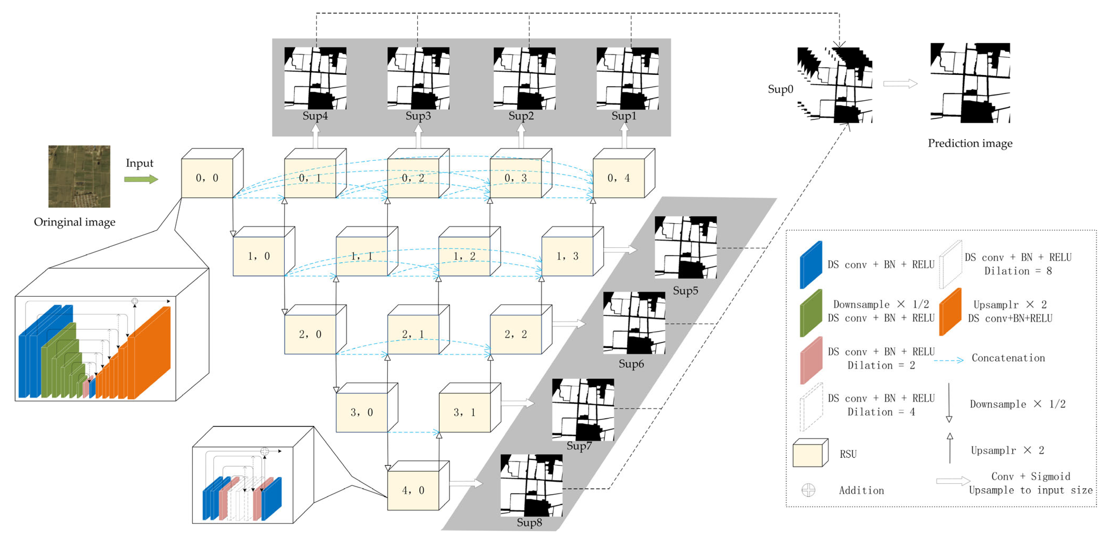
The overall framework of the designed farmland extraction model, U-Net++, is shown in Figure 3. U2-Net++ consists of an input layer; several nested, densely connected RSU modules that process and aggregate the outputs at different stages; and an attention module that generates a farmland area map. There are 15 stages, represented by the squares in the figure below, each of which is filled with a well-configured RSU module. Dense skip connections are nested between RSU modules. Therefore, multiscale features and multiscale diagnoses can be extracted within the stage. The depth of each RSU module in the horizontal direction is consistent, with depth L of the (0, x) module being 7, depth L of the (1, x) module being 6, depth L of the (2, x) module being 5, and depth L of the (3, x) module being 4. The (4, 0) module does not continue to downsample because the resolution of the input feature map is relatively low, and further reduction in these feature maps would result in the loss of useful context. L is typically configured based on the spatial resolution of the input feature map. For feature maps with large heights and widths, a larger L value was used to capture large-scale information.
In the vertical direction of the encoding process, downsampling was performed each time it ran downward, thereby reducing the size of the feature map by half. If our original input image is 512 × 512 pixels, the feature map obtained after passing through the (0, 0) module is 512 × 512 pixels. Before entering the (1, 0) module, downsampling was performed to obtain a feature map of 256 × 256 pixels. Conversely, in the vertical direction of the decoding process, upsampling was performed using bilinear interpolation to upsample the feature map to its original size. In the horizontal direction, the input of the next RSU module receives the feature map that has been upsampled by the lower module in the vertical direction and all previous steps in the horizontal direction and concatenates them. The input of module (0, 3) was obtained by upsampling the output feature map of module (1, 2) and concatenating it with the output feature maps of (0, 0), (0, 1), and (0, 2). The complete image size change process is shown in Table 1.
Given that our designed model uses more RSU modules and more feature maps in the process, we recorded the channel numbers (“I”, “M”, and “O” represent the number of input channels (Cin), intermediate channels, and output channels (Cout) of each block, respectively) of the feature maps during the process. The complete channel number change process is shown in Table 2.
A probability map fusion module was used to generate the field block probability map. In the model design, we input the feature map output using the outermost RSU module of U2-Net++ into the spatiotemporal attention mechanism module. We then used a 3 × 3 convolutional layer and sigmoid function to output field block probability maps S(8), S(7), S(6), S(5), S(4), S(3), S(2), and S(1) from stages (0, 1), (0, 2), (0, 3), (0, 4), (4, 0), (3, 1), (2, 2), and (1, 3). These probability maps were then fused through cascading operations to obtain S(0), and a 1 × 1 convolutional layer and sigmoid function were used to generate the final saliency probability mapping.

2.3.1. RSU Structure

Residual Split-Upsampling (RSU) is a module that consists of three parts, namely, the Residual Block, the Split Block, and the Upsampling Block, similarly to the U-Net used for image segmentation. This can gradually perform downsampling, upsampling, and concatenation operations on the input feature map to extract multiscale information.
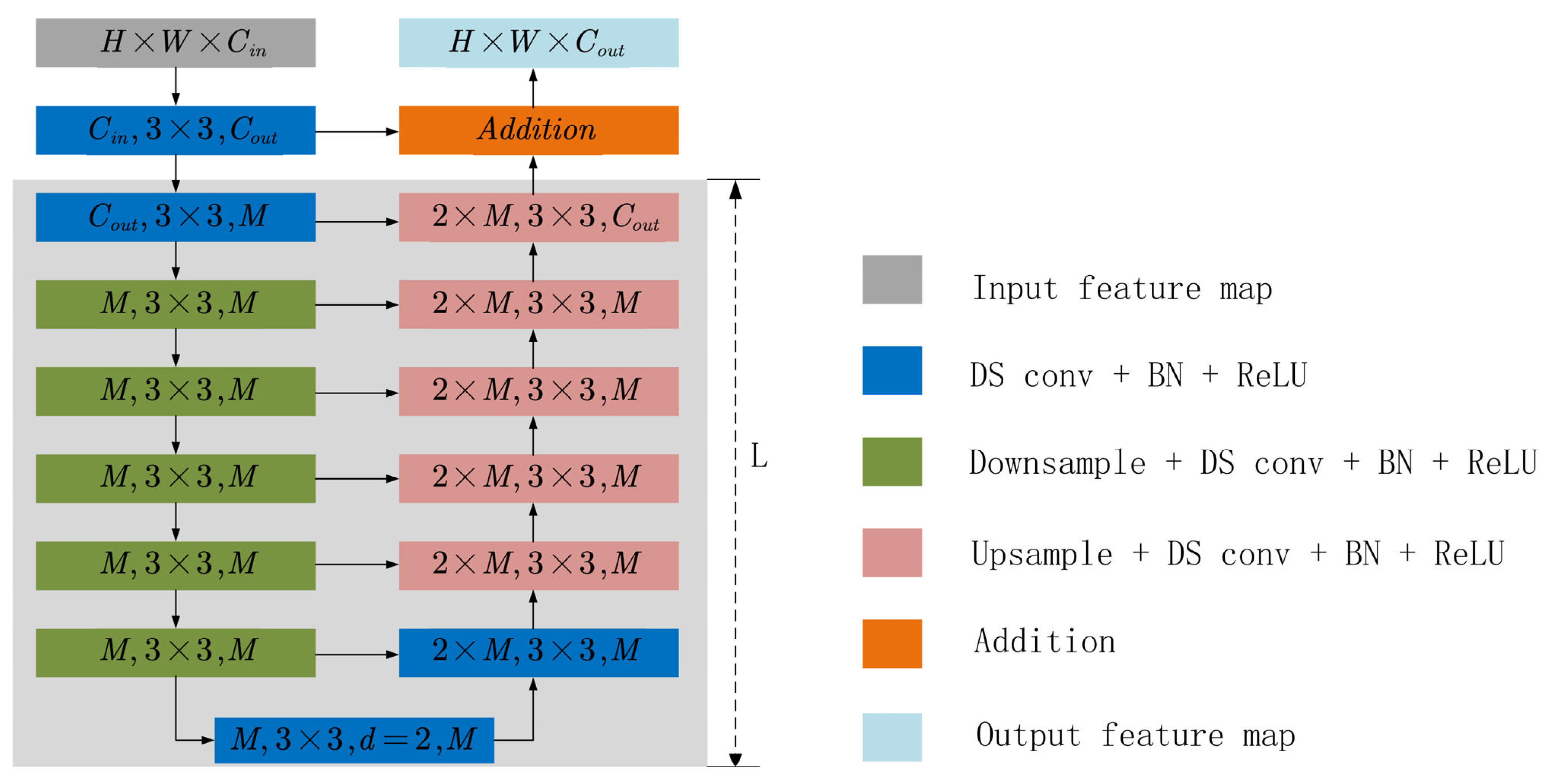
The Residual Block is used to extract multilevel features, including operations such as convolution, batch normalization, and activation, and its structure is shown in Figure 4. The Split Block extracts high-level features through parallel convolution, further separating different feature representations. The Upsampling Block upsamples the low-resolution feature map to the original resolution through transposed convolution and merges the high-resolution feature map with the low-resolution feature map through skip connections to extract more comprehensive multiscale information. In recent convolutional neural networks, small convolution filters (1 × 1 or 3 × 3) such as VGG, ResNet, and ResU-Net have been widely used for feature extraction because of their small size. However, because our model is deeper and has more parameters than U2-Net, we applied a depth-wise separable convolution to our model to speed up the training process (Figure 5). The three most important parts of the RSU module are as follows:
(1)
The input convolution layer was used for local feature extraction by converting the input feature map x (H × W × Cin) into an intermediate feature map F1(x) with Cout channels. This is a typical convolutional layer that is used for local feature extraction.
(2)
The model has a symmetrical encoder–decoder structure similar to U-Net with a height of L, taking the intermediate feature map F1(x) as the input to learn to extract and encode multiscale contextual information U(F1(x)), where U denotes the U-net structure. A larger L results in deeper U-blocks (RSUs), more pooling operations, a larger receptive field range, and richer local and global features. By configuring this parameter, multiscale features can be extracted from input feature maps at any spatial resolution. Multiscale features were extracted from the gradually downsampled feature maps and encoded into high-resolution feature maps through progressive upsampling, concatenation, and convolution. This process alleviated the loss of detail caused by large-scale upsampling.
The model performs more effectively with the U-Net structure for multiscale feature extraction and encoding, where the L parameter determines the depth of the model and the range of the receptive field. Meanwhile, gradual downsampling and progressive upsampling, concatenation, and convolution processes help alleviate the loss of details caused by direct upsampling.
(3)
Local and multiscale features are fused through residual connections, that is, HRSU(x) = U(F1(x)) + F1(x).

2.3.2. Depth-Wise Separable Convolution

Depth-wise separable convolution (Figure 5) is a convolution operation that decomposes a standard convolution operation into two steps, significantly reducing the computational complexity and number of parameters while maintaining a certain level of accuracy. This is because depth-wise separable convolution decomposes the convolution operation into two steps, that is, channel-wise and point-wise.
In the channel-wise convolution (Figure 5a) stage, each input channel has an independent spatial filter applied to all the spatial positions of each channel, which generates a feature map. Subsequently, point-wise convolution convolves (Figure 5b) the feature map to transform the feature map produced by the depth-wise convolution into a new feature space. Depth-wise separable convolution reduces the computational cost because each input channel has an independent spatial filter, which reduces the amount of computation required for convolution. In point-wise convolution, the size of the convolution kernel was 1 × 1, which significantly reduced the number of parameters.
Depth-wise separable convolution has been shown to perform well in various computer vision tasks such as image classification, object detection, and semantic segmentation. In addition, depth-wise separable convolution is an important component of modern deep learning architectures such as MobileNet and Xception.

2.3.3. Spatial-Channel Attention Mechanism

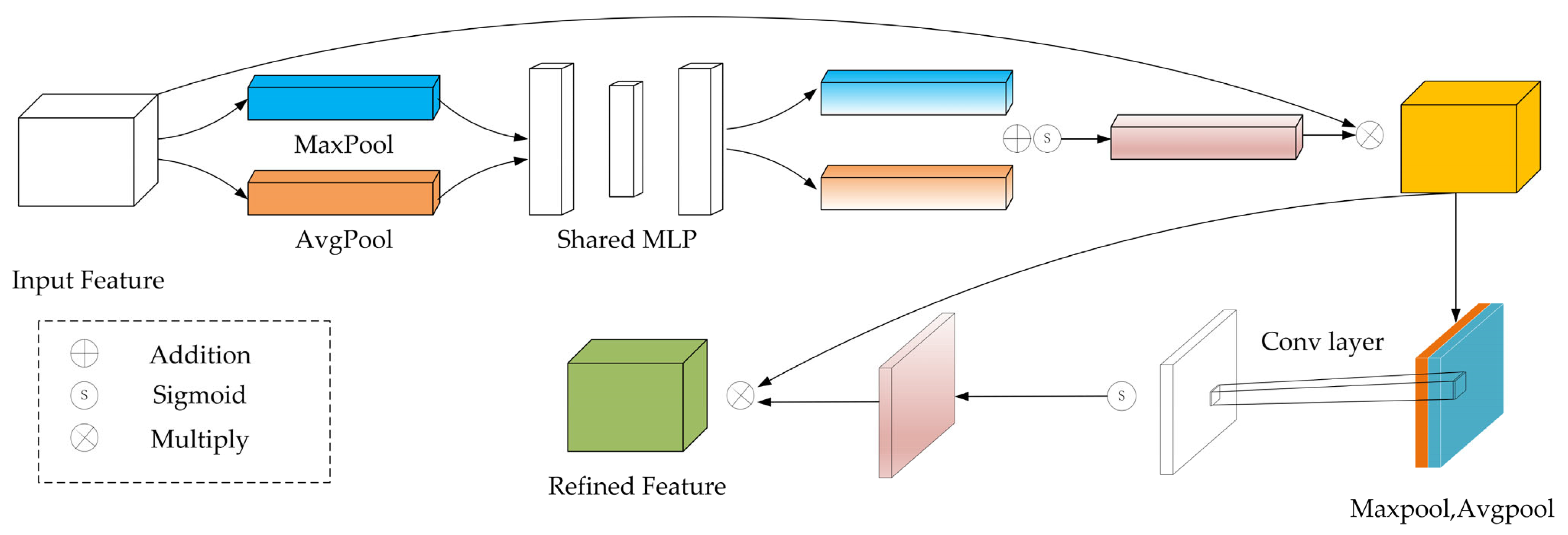
The CBAM (Convolutional Block Attention Module) is an attention mechanism for convolutional neural networks (CNNs) that can adaptively learn the feature representations of different regions in an image. The CBAM consists of two modules, that is, the Channel Attention Module and the Spatial Attention Module. The Channel Attention Module adapts to the importance of each channel by learning the relationships between the different channels. This module captures global information between channels through global average-pooling and global max-pooling operations. It then processes this information through two fully connected layers and an activation function to generate channel weights. The channel weights were multiplied by the feature map of each channel to produce an adaptive feature representation. The structure of the spatial-channel attention mechanism is shown in Figure 6.
The Spatial Attention Module adaptively adjusts the importance of each position by learning the relevance of each spatial location in the image. This module uses a series of convolutional and pooling operations to capture spatial information in the image. It then processes this information through two fully connected layers and an activation function to generate position weights. The position weights were multiplied by the feature map at each position to produce an adaptive feature representation.

2.3.4. Loss

During the training process, our model’s prediction results not only included the final field block prediction map but also eight feature maps of different scales from S(1) to S(8). Therefore, when training the model, we supervised not only the final output map of the network but also the feature maps of different scales in the middle. To achieve this goal, we used a depth supervision method similar to the holistic nested-edge detection (HED, Equation (1)) method [37], outputting eight losses for each iteration. These losses were used to adjust the model parameters to minimize errors and accurately depict the overlapping field blocks.
L = m = 1 M w s i d e ( m ) l s i d e ( m ) + w f u s e l f u s e
Among these, l s i d e ( m ) (M = 8, Sup1–8 in Figure 3 above) is the loss of the side-output saliency map, and S s i d e ( m ) and l f u s e are the losses of the final fused output saliency map. w s i d e ( m ) and l f u s e are the weights of each lost item. For each term l, we use the standard binary cross-entropy function to calculate the loss, as shown in Equation (2):
L = ( i ,   j ) ( H ,   W ) [ P G ( i ,   j ) log P S ( i ,   j ) + ( 1 P G i ,   j ) log ( 1 P S ( i ,   j ) ) ]
where ( i ,   j ) are the pixel coordinates and ( H ,   W ) are the image size, height, and width, respectively. P G ( i ,   j ) and P S ( i ,   j ) represent the pixel values of the true value and the predicted saliency probability map, respectively. The training process attempts to minimize the overall loss L (Equation (1)). The fused output l f u s e was selected as the final saliency map during the testing process.

2.4. Accuracy Evaluation

Intersection over Union ( I o U , Equation (3)) is a metric used to evaluate the prediction results of models in tasks such as object detection and semantic segmentation. It measures the degree of overlap between the predicted result and the true target, where R and P represent the regions predicted by the model and the true target region, respectively. The comparison between the true category of the sample and the prediction result of the model can be divided into four situations, that is, True Positive ( T P ), where the predicted value of the olive crown is consistent with the true value; False Positive ( F P ), where the actual situation is the background but is mistakenly predicted as a crown; False Negative ( F N ), where the crown in the real scene is not correctly recognized; and True Negative ( T N ), where the background is consistent with the true value. Precision (Equation (4)), recall (Equation (5)), overall accuracy ( O A , Equation (6)), and F 1 S c o r e (Equation (7)) were used as indicators to evaluate the model. The higher the precision, recall, O A , and F 1 S c o r e , the closer the predicted value is to the true value.
I o U = | R     P R   P |
P r e c i s i o n = T P T P + F P
R e c a l l = T P T P + F N
O A = T P + T N T P + F P + T N + F N
F 1 S c o r e = 2 × P r e c i s i o n × R e c a l l   P r e c i s i o n + R e c a l l  

3. Results

The software and hardware parameters used in this study are shown in Table 3. Although we designed a relatively deep network structure owing to the design of the RSU block and the use of a depth-separable convolution, our model does not require a large amount of computational power. We randomly split the dataset into three subsets (training, validation, and test) according to different types of plots with a ratio of 8:1:1. Each subset contains data from all three plot types. We used the training and validation subsets for model training, and the test subset did not participate in the training process. During the training process, we used data augmentation, such as random cropping and rotation of the input image, and the AdamW [38] optimizer to adjust the model training process. The batch size of the model was set to four, the number of iterations was 360, and other hyperparameters were set to default values, that is, the learning rate was 0.001, the weight decay was 1 × 10⁻⁴, and the evaluation interval was 10. According to the given parameters for configuration training, we input our samples for iterative training, which required 14 h.

3.1. CBAM and Depth-Separable Convolution Performance Deviation

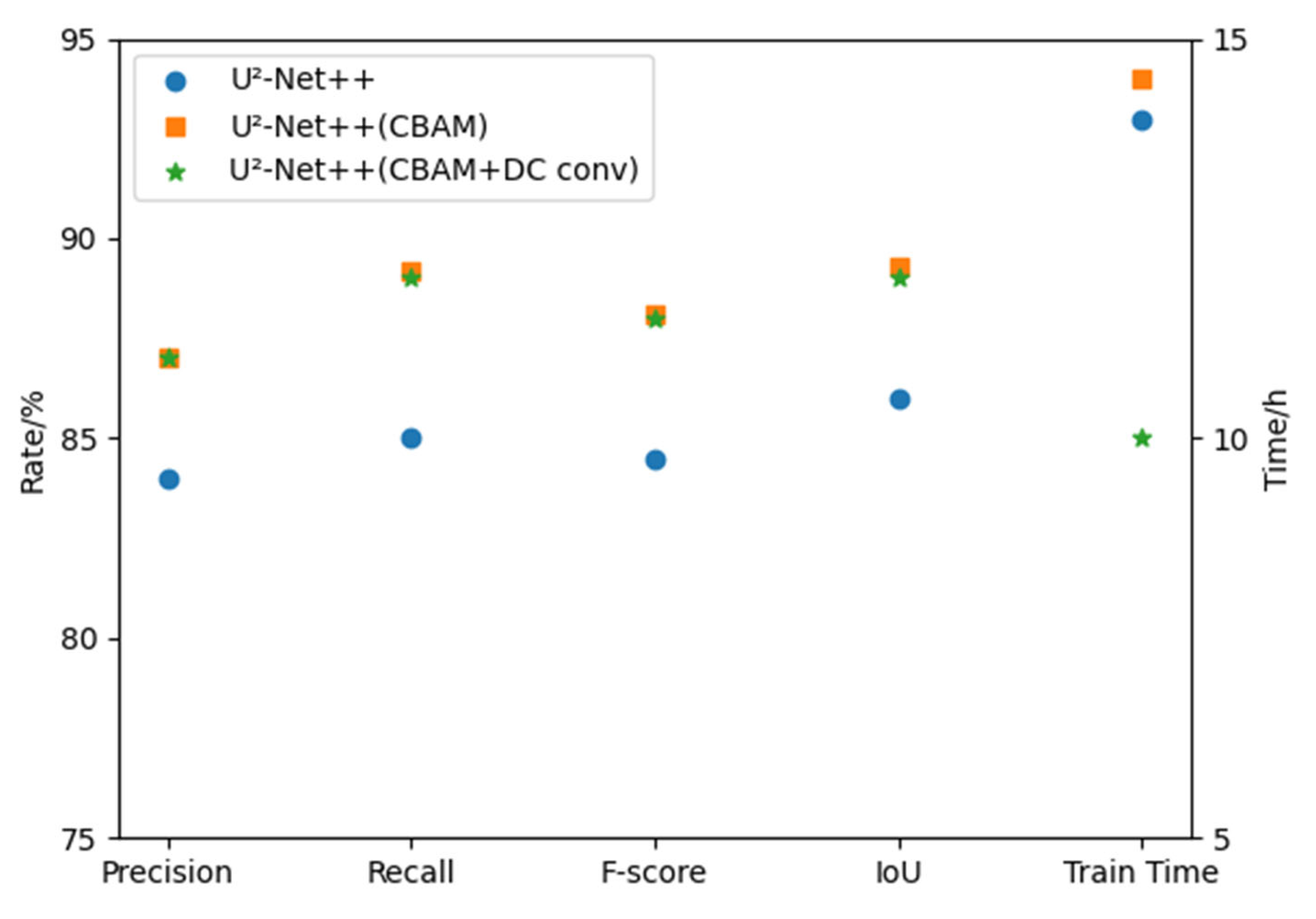
To evaluate the impact of separable convolution and the spatial-channel attention mechanism on the model’s performance, we tested the results of field extraction and training speed before and after adding these two methods to our model. We used U2-Net++ to test the performance of the models using traditional and separable convolutions. The results showed that after using depth-separable convolution, the accuracy of the model could be maintained, with the accuracy of precision, recall, F1-score, and IoU fluctuating within ±1%. However, the training speed was reduced by 4 h. This demonstrated that depth-separable convolution plays an important role in convolutional neural networks, thereby significantly reducing the time required for training while ensuring accuracy.
The time required for training did not significantly change after the addition of the spatial-channel attention mechanism. The time required to train our data before adding it was 14 h, and the time required after adding it was 14.5 h. However, for the four indicators, the accuracy improved to varying degrees. The precision increased by 3.05%, the recall increased by 4.21%, the F1-score increased by 3.63%, and the IoU increased by 3.31%. The data plot is shown in Figure 7. Therefore, the spatial-channel attention mechanism improved the accuracy of field extraction.

3.2. Extract Effects from Different Areas

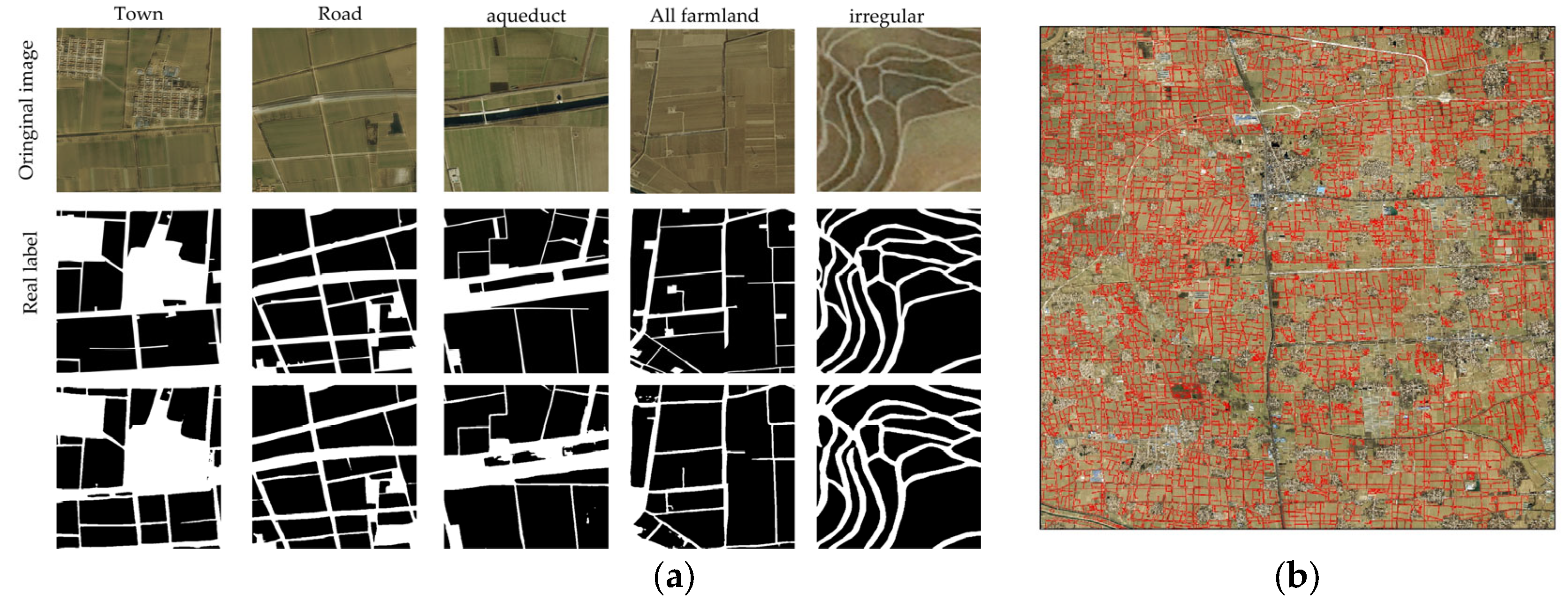
We used our U2-Net++ model to extract fields from different regions, as shown in Figure 8. Figure 8 shows that the extraction effect worked successfully in all test areas. In areas where towns and farmlands intersected, the proportion of farmland was relatively small, and the boundary was adjacent to buildings. Some fields did not have prominent ridges. However, our model could still extract clear outlines of the fields, which were consistent with the actual shape. In areas where roads and farmland intersected, our model was not affected by the road and could accurately extract the field boundary. In areas where the canal and farmland intersected, the extraction effect of small fields on the side of the canal was not as effective as in other areas. We concluded that this was because our sketched samples contained less content. In areas where an entire field was present, our model had the strongest extraction effect, and the field boundary was complete. The boundary of the irregular plot area is extracted completely and realistically by our model. In all divisions, we did not have a “misclassification” situation, that is, areas that are not fields extracted as fields, and the accuracy rate was relatively high. This was a situation of “missing points.” Given our limited manpower, the number of samples drawn was relatively small, and there were many actual situations such as these in the fields. Therefore, our samples did not contain all the information, resulting in a “missing point” situation.
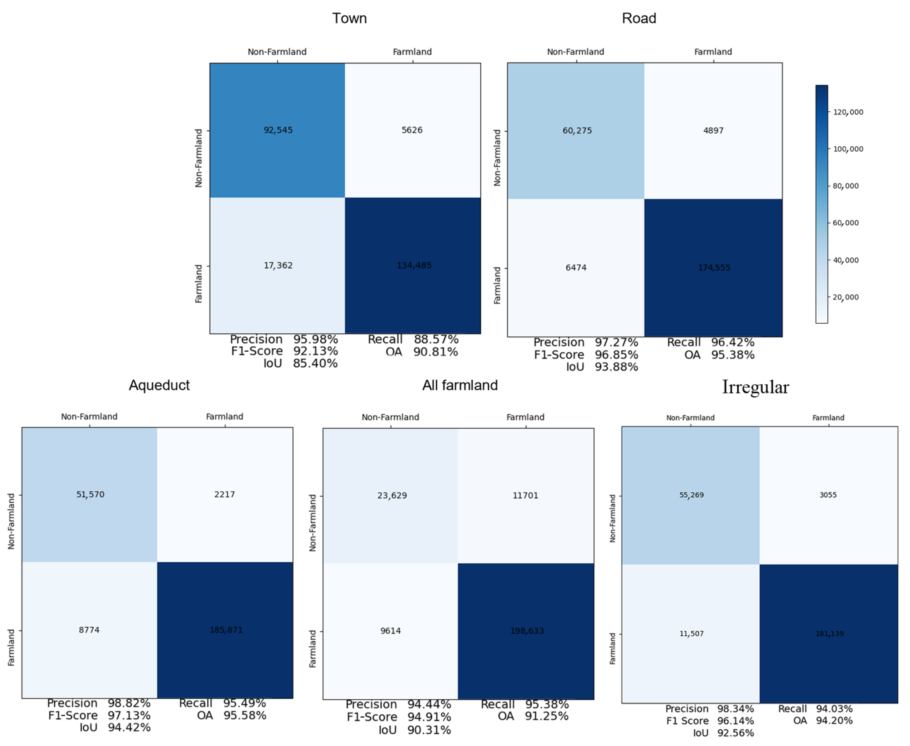
The results of the quantitative evaluation of our model’s farmland extraction under different scenarios are shown in Figure 9. Scenario 1 indicates farmland extraction alongside the town, whereas Scenarios 2, 3, and 4 indicate farmland extraction along the road, aqueduct, and all farmlands, respectively. We observed a high level of precision (>94.44%) for all the scenarios. The accuracy rate and F1-score were also significant across towns, roads, aqueducts, and all farmlands, with values greater than 90.81% and 92.13%, respectively.
An analysis of the accuracy of farmland extraction under different scenarios showed that the boundaries of farmland around cities were not smooth, and there were errors in boundary recognition and unrecognized situations. The highest rate of precision (98.82%) was achieved using this model for farmland extraction along the channel. This was followed by irregular (98.43%) farmland extraction along roads (97.27%), towns (95.98%), and all farmlands (94.44%) (Figure 9). The highest accuracy rate for this model was also observed for farmland extraction along the channel, whereas the lowest was observed for farmland extraction alongside the town (Figure 9). The same trend was observed for the F1-score, OA, and IoU values. The higher precision, accuracy level, and F1-score values for Scenarios 3 and 2 indicated that the extraction efficiency was less affected by roads and canals. The entire scenario showed that our model had a high level of applicability under all given conditions (Figure 9).

3.3. Performance Evaluation of Different Deep Learning Models

To study the applicability of the U2-Net++ model, the extraction results were compared with those of other mainstream deep learning models for image segmentation, that is, FCN, U-Net, Deeplabv-3, and U2-Net. These models used the same training method as U2-Net++, did not use pretrained weights, and used our sample data for training. The test visualization extraction results are presented in Figure 10. In the same experimental area, the extraction effects of several deep learning models did not show pronounced misclassification. This indicated that these models could effectively distinguish the target features from background features. However, in areas with only farmland and where roads and farmland intersected, FCN, U-Net, and SegNet had severe overall omissions, poor extraction integrity, and severe noise. The extraction results of the Deeplabv-3 and U2-Net models were more accurate than those of U-Net and FCN overall. However, there were still omissions and noise, especially in areas where the boundaries of farmland were less prominent, such as around cities. The U2-Net++ model used in this study significantly reduced misclassifications and omissions. Although some defects still occurred, the effects of the farmland boundary segmentation were relatively positive. Although there were still small boundaries around cities and some noise, the U2-Net++ model used in this study significantly reduced misclassification and omission and had a positive effect on farmland extraction.
The results of the quantitative analysis of the extraction accuracy of several models are listed in Table 4. There were differences in the performances of several algorithms for the five indicators of precision, recall, F1-score, OA, and IoU. U2-Net++ performed well for all the indicators, demonstrating its superiority in image segmentation tasks. U2-Net++ achieved an impressive accuracy of 98.82%, which is a significant improvement over the highest competing models, that is, FCN and SegNet (97.04%). The accuracy of U2-Net++ was nearly 10 percentage points higher than that of U-Net (89.54%). This indicates that the model could accurately identify and classify pixels and minimize misclassifications. A high level of accuracy is an important indicator of a model in image segmentation applications because it is directly related to the classification ability and accuracy of the model.
In terms of recall, U2-Net++ also performed successfully, reaching 95.49%, which is an improvement over the highest competing models, that is, DeepLabv3+ (92.99%) and U2-Net (93.99%). By contrast, the U-Net recall rate (72.20%) was significantly lower than that of U2-Net++. This indicates that the model could effectively detect and recover target areas in the true segmentation mask. A high recall is important for image segmentation tasks because it ensures the integrity and accuracy of the target area.
The F1-score is an important indicator that considers both precision and recall to evaluate the overall performance of the model. U2-Net++ achieved a satisfactory F1-score of 97.13%, surpassing those of the competing models, DeepLabv3+ (95.185%) and U2-Net (95.49%). In contrast, the F1-score of U-Net (79.50%) was significantly lower than that of the U2-Net++ group. This indicates that the model achieved an appropriate balance between accuracy and recall and maintained a high recall rate while maintaining high accuracy.
In addition to its advantages in terms of individual indicators, U2-Net++ performed well in terms of overall accuracy (OA) and IoU. The overall accuracy was 95.58%, indicating the classification accuracy of the model for the entire image. The IoU reached 94.42%, indicating that U2-Net++ could produce segmentation results that strongly overlapped with the true segmentation mask, further demonstrating its accuracy and reliability.
In terms of computational cost, we trained all models using the same dataset and hyperparameters. The total training time of relatively simple models such as U-Net and FCN with low segmentation accuracy was about 8 h, while the total training time of the DeepLabv3+, U2-Net, and U2-Net++ models with high accuracy was about 10 h. Among them, SegNet had the shortest training time, which took 7.06 h; U2-Net++ had the longest training time, which took 10.12 h. The computing cost of U2-Net++ was 3.48% higher than that of U2-Net and 2.95% higher than that of DeepLabv3+.
Overall, U2-Net++ achieved significant improvements in precision, recall, and F1-score compared with the other models. Compared with the most accurate competing model, the precision of U2-Net++ increased by approximately 1.78 percentage points, the recall increased by approximately 1.5 percentage points, and the F1-score increased by approximately 1.36 percentage points. These improvements indicate that U2-Net++ had a higher level of accuracy and reliability in pixel classification and target area recovery.

3.4. Applicability of Different Resolutions in Different Regions

To validate the applicability of our model, it was applied to areas with three different types of cultivated land. The results have demonstrated that our model performed effectively in extracting cultivated land blocks across diverse land types. Despite the varying influencing factors in different cultivated land types, our model exhibited robustness in handling these challenges. The adaptability of our model to different regions and distinct conditions has demonstrated its versatility and effectiveness. The ability to effectively extract cultivated land blocks from diverse areas and land cover types reinforces the reliability and generalizability of our model, making it a valuable tool for land use and agricultural planning.

3.4.1. Dryland in Northern China (Gaoqing County)

The partial view in Figure 11 shows that our model not only detected the boundaries of cultivated land but also performed successfully in detecting other boundary types, such as residential areas, roads, canals, and forest boundaries. However, these non-cultivated areas, particularly forest regions, caused some interference in the detection of the model. This was because of the similarity in color and texture between forest and cultivated land during image capture, which affected the extraction accuracy.
Some rivers were misidentified as cultivated land. This could be attributed to the high sediment content in the downstream area of the Yellow River, resulting in a similar appearance to that of cultivated land in the imagery. Given that our model performs inferences after cropping the images, the size of the cropped images sometimes causes the model to mistakenly interpret certain river sections as large, cultivated land blocks.
Overall, our model exhibited high precision in the extraction results for the northern dryland region, displaying clarity in the boundaries and completeness in the land parcel extraction.

3.4.2. Paddy Fields in Southern China (Suxicheng District)

The overall view in Figure 12 shows that the distribution of paddy field blocks extracted by the model aligns with the actual distribution in the southern region. The extraction results for planted and unplanted areas had a high level of performance with clear and complete boundaries, validating the accuracy of the extraction algorithm.
However, in certain areas, the extraction accuracy of paddy fields decreased slightly. This was because of the presence of residential areas and thin clouds in the imagery. The accuracy of the paddy field extraction was particularly affected in small block areas within residential regions. This may be because of image artifacts caused by clouds, leading to limitations in the edge-detection algorithm. A spatial distribution analysis of the extracted paddy fields highlighted a certain degree of spatial aggregation in terms of size and shape. This suggests that, in specific regions, farmers tended to have relatively larger and more regular-shaped paddy fields, which was likely influenced by local land use policies and agricultural practices.

3.4.3. Terraced Fields in Southwestern China (Yuanyang County)

The extraction outcome was highly satisfactory despite the narrow and elongated terraced fields. In the extracted images of the terraced fields shown in Figure 13, the cultivated land blocks appear to be complete and accurate, and the extracted terraced field boundaries closely align with the ground truthing from the field surveys, confirming the accuracy of the algorithm.
However, the extraction results were limited to areas with steep slopes. We found that this limitation was because of the small proportion of terraced fields in the imagery. This meant that it was challenging to accurately determine the boundaries. Consequently, the performance of the model was constrained in such areas. Overall, the model demonstrated excellent extraction results for terraced fields with high accuracy and precision and performed well in most terraced field areas. However, there may be limitations in regions with substantial slopes and small proportions of cultivated land.

4. Discussion

This study proposes a method for using the U2-Net++ model in combination with remote sensing data for field extraction, with the aim of achieving efficient and accurate field boundary extraction and area estimation. The results have shown that this method has considerable advantages and importance in field extraction tasks and is capable of meeting the demand for field information in agricultural management and land use planning. Compared with traditional manual measurement methods, the method using the U2-Net++ model in combination with remote sensing data has many advantages. Traditional manual measurement methods require a substantial amount of time and human resources and are prone to errors. By using the U2-Net++ model in combination with remote sensing data, automatic field extraction could be achieved, with improved efficiency and data processing accuracy. Traditional manual measurement methods have difficulties with real-time monitoring and cannot be used to obtain timely information on field boundaries and areas. By using the U2-Net++ model in combination with remote sensing data, high spatiotemporal resolution image data could be obtained through unmanned aerial vehicle remote sensing platforms, enabling real-time monitoring and updating of fields and providing reliable data support for agricultural management and decision-making.
As a deep learning algorithm, the U2-Net++ model has a high level of accuracy and generalization ability in processing remote sensing data. Compared with traditional machine learning algorithms, U2-Net++ can extract deep, non-linear feature information from complex remote sensing images, making the field extraction results more accurate and stable. Therefore, using the U2-Net++ model in combination with remote sensing data provides a more reliable and efficient solution for agricultural management tasks, such as field boundary extraction and area estimation.
We tested the newly built U2-Net++ model based on the RSU module and compared the effectiveness of several different deep neural networks for field extraction, including U-Net, FCN, U-Net++, SegNet, DeepLabv3+, and U2-Net. Our results show that the U2-Net++ model performs well in terms of field extraction accuracy. Compared with older algorithms, the U2-Net++ model improved the F1-score by 7.36% to 17.63%. Compared with more advanced and complex models (DeepLabv3+, U2Net), it was also improved by more than 2%. This indicates that the U2-Net model could acquire more accurate extraction results in a field with fewer data and more complex scenarios. We evaluated the impact of depth-wise separable convolution and spatial-channel attention mechanisms on model performance. The results show that after using depth-wise separable convolution, the model accuracy could be maintained, and the training time could be reduced by 4 h. The training time did not change significantly before and after the addition of the spatial-channel attention mechanism. However, the accuracy improved to varying degrees. These results demonstrate that our model has a high level of ability to extract fields and meet the requirements of improving field survey efficiency, achieving precise agricultural management, improving farmers’ production conditions, protecting the ecological environment, and promoting local economic development. Despite some achievements in our research, there were some limitations. The number of samples used was relatively small and may not encompass all situations. In addition, we only tested a few deep learning models; therefore, more models should be considered in future research.
In summary, this study demonstrates that deep learning methods have strong application prospects for field extraction. However, our method has some limitations that require improvement:
(1)
Although the proposed model has been proven to be accurate and effective, it has certain limitations. Analyzing the results showed that when the image contained unclear field boundaries, boundaries obscured by trees or shadows, large changes in crops within the field, or irregular field shapes, the extracted field boundaries were unclear. However, this was to be expected because, combined with human observation, the boundaries of the fields were less visible. Trees and shadows could cause changes in the color of an image, which could prevent the model from detecting the field or generating curved boundaries that are not conducive to engineering applications. There are some post-processing methods for obtaining smoother boundaries, but this is not in line with our original intention for the use of deep learning. Despite these issues, we were still able to extract the field boundaries effectively.
(2)
The images used in this study were obtained in the winter and spring. During this period, no crops were planted in the fields, which is why we chose to extract more accurate field boundaries and minimize the impact of other factors on the extraction results. However, if there are no corresponding high-resolution images of the area where the field must be extracted during this period, it is difficult to continue this work. The samples used for training were all bare soil. Therefore, they would not have a positive effect on images with crops. If the images of bare soil and crops were trained together, the model would not achieve the highest accuracy in both scenarios. Therefore, the proposed method trains different weights for different regions and seasons for engineering applications. This still requires a substantial amount of work. Therefore, follow-up research will be conducted from the aspect of samples and models to ensure that all fields can be extracted with a complete set of sample sets.

5. Conclusions

In this study, we used high-resolution remote sensing imagery (GF-7, ZY-3, and Google Earth images) to create samples of cultivated land blocks. We developed a deep learning model known as U2-Net++ for the automatic extraction of selected cultivated land blocks using the RSU module, depth-wise separable convolution, and spatial-channel attention mechanism. The results of the cultivated land block extraction demonstrated that the U2-Net++ model exhibited exceptional precision. Compared with several older algorithms, the U2-Net++ model achieved the highest scores in terms of recognition accuracy, recall rate, and F1-score, with improvements ranging from 7.36% to 17.63%. When compared with more complex and advanced models, such as DeepLabv3+ and U2-Net, the U2-Net++ model showed an improvement of over 2%.
We generated large-scale maps for three different types of cultivated land, that is, drylands, paddy fields, and terraced fields, all of which displayed high accuracy, confirming the applicability of our model. By combining the U2-Net++ model with remote sensing data, our approach provides a reliable and efficient solution for tasks such as cultivated land boundary extraction and area estimation, thereby contributing to more effective agricultural management.

Author Contributions

Conceptualization, C.L. and S.W.; methodology, C.L., S.W. and S.T.; software, C.L., S.W. and L.Y.; validation, C.L., S.W. and L.H.; formal analysis, C.L., L.H. and G.R.; investigation, C.L., L.H. and G.R.; resources, C.L., F.T. and H.Q.; data curation, C.L., L.S. and L.J.; writing—original draft preparation, C.L.; writing—review and editing, C.L., S.W., L.Y., J.W. and H.A.; visualization, C.L. and M.L.; supervision, C.L., S.W. and L.Y.; project administration, S.W., L.Y. and L.H.; funding acquisition, S.W. All authors have read and agreed to the published version of the manuscript.

Funding

This research was funded by the Jiangsu Water Conservancy Science and Technology Project (2021081); the Hunan Province Water Conservancy Science and Technology Project “Research and Application of Key Technologies for Remote Sensing Monitoring and Evaluation of Flood Control and Drought Control in Hunan Province”; the Three Gorges Follow-up Work “Remote Sensing Investigation and Evaluation of Flood Control Safety in the Three Gorges Section”; the Basic scientific research business fund of the Chinese Academy of Water Sciences (JZ110145B0012021); and the key technology research of the “four precautions” intelligent platform for flood and drought disaster prevention in River Basin Digital Twinning.

Data Availability Statement

The dataset analyzed in this study is managed by the China Institute of Water Resources and Hydropower Research. The dataset can be made available upon request from the corresponding authors.

Conflicts of Interest

The authors declare no conflict of interest.

References

  1. Haworth, B.T.; Biggs, E.; Duncan, J.; Wales, N.; Boruff, B.; Bruce, E. Geographic Information and Communication Technologies for Supporting Smallholder Agriculture and Climate Resilience. Climate 2018, 6, 97. [Google Scholar] [CrossRef]
  2. Jain, M.; Singh, B.; Srivastava, A.A.K.; Malik, R.K.; McDonald, A.J.; Lobell, D.B. Using Satellite Data to Identify the Causes of and Potential Solutions for Yield Gaps in India’s Wheat Belt. Environ. Res. Lett. 2017, 12, 094011. [Google Scholar] [CrossRef]
  3. Neumann, K.; Verburg, P.H.; Stehfest, E.; Müller, C. The Yield Gap of Global Grain Production: A Spatial Analysis. Agric. Syst. 2010, 103, 316–326. [Google Scholar] [CrossRef]
  4. Wagner, M.P.; Oppelt, N. Extracting Agricultural Fields from Remote Sensing Imagery Using Graph-Based Growing Contours. Remote Sens. 2020, 12, 1205. [Google Scholar] [CrossRef]
  5. Persello, C.; Tolpekin, V.A.; Bergado, J.R.; de By, R.A. Delineation of agricultural fields in smallholder farms from satellite images using fully convolutional networks and combinatorial grouping. Remote Sens. Environ. 2019, 231, 111253. [Google Scholar] [CrossRef] [PubMed]
  6. Zhao, W.Z.; Du, S.H.; Emery, W.J. Object-based convolutional neural network for high-resolution imagery classification. IEEE J. Sel. Top. Appl. Earth Obs. Remote Sens. 2017, 10, 3386–3396. [Google Scholar] [CrossRef]
  7. Blaschke, T. Object based image analysis for remote sensing. ISPRS J. Photogramm. Remote Sens. 2010, 65, 2–16. [Google Scholar] [CrossRef]
  8. Matton, N.; Canto, G.; Waldner, F.; Valero, S.; Morin, D.; Inglada, J.; Arias, M.; Bontemps, S.; Koetz, B.; Defourny, P. An automated method for annual cropland mapping along the season for various globally- distributed agrosystems using high spatial and temporal resolution time series. Remote Sens. 2015, 7, 13208–13232. [Google Scholar] [CrossRef]
  9. Marvaniya, S.; Devi, U.; Hazra, J.; Mujumdar, S.; Gupta, N. Small, sparse, but substantial: Techniques for segmenting small agricultural fields using sparse ground data. Int. J. Remote Sens. 2021, 42, 1512–1534. [Google Scholar] [CrossRef]
  10. Turker, M.; Kok, E.H. Field-based sub-boundary extraction from remote sensing imagery using perceptual grouping. ISPRS J. Photogramm. Remote Sens. 2013, 79, 106–121. [Google Scholar] [CrossRef]
  11. Yan, L.; Roy, D.P. Automated crop field extraction from multi- temporal Web Enabled Landsat Data. Remote Sens. Environ. 2014, 144, 42–64. [Google Scholar] [CrossRef]
  12. Cheng, T.; Ji, X.S.; Yang, G.X.; Zheng, H.; Ma, J.; Yao, X.; Zhu, Y.; Cao, W. DESTIN: A new method for delineating the boundaries of crop fields by fusing spatial and temporal information from WorldView and Planet satellite imagery. Comput. Electron. Agric. 2020, 178, 105787. [Google Scholar] [CrossRef]
  13. Evans, C.; Jones, R.; Svalbe, I.; Berman, M. Segmenting multispectral Landsat TM images into field units. IEEE Trans. Geosci. Remote Sens. 2002, 40, 1054–1064. [Google Scholar] [CrossRef]
  14. Watkins, B.; van Niekerk, A. Automating field boundary delineation with multi- temporal Sentinel-2 imagery. Comput. Electron. Agric. 2019, 167, 105078. [Google Scholar] [CrossRef]
  15. García-Pedrero, A.; Gonzalo-Martín, C.; Lillo-Saavedra, M. A machine learning approach for agricultural parcel delineation through agglomerative segmentation. Int. J. Remote Sens. 2017, 38, 1809–1819. [Google Scholar] [CrossRef]
  16. Chen, B.; Qiu, F.; Wu, B.; Du, H. Image Segmentation Based on Constrained Spectral Variance Difference and Edge Penalty. Remote Sens. 2015, 7, 5980–6004. [Google Scholar] [CrossRef]
  17. Belgiu, M.; Csillik, O. Sentinel-2 cropland mapping using pixel-based and object-based time-weighted dynamic time warping analysis. Remote Sens. Environ. 2018, 204, 509–523. [Google Scholar] [CrossRef]
  18. Crommelinck, S.; Bennett, R.; Gerke, M.; Yang, M.Y.; Vosselman, G. Contour Detection for UAV-Based Cadastral Mapping. Remote Sens. 2017, 9, 171. [Google Scholar] [CrossRef]
  19. Masoud, K.M.; Persello, C.; Tolpekin, V.A. Delineation of Agricultural Field Boundaries from Sentinel-2 Images Using a Novel Super-Resolution Contour Detector Based on Fully Convolutional Networks. Remote Sens. 2020, 12, 59. [Google Scholar] [CrossRef]
  20. Xu, W.; Deng, X.; Guo, S.; Chen, J.; Wang, X. High-Resolution U-Net: Preserving Image Details for Cultivated Land Extraction. Sens. Multidiscip. Digit. Publ. Inst. 2020, 20, 4064. [Google Scholar] [CrossRef]
  21. Waldner, F.; Diakogiannis, F.I. Deep Learning on Edge: Extracting Field Boundaries from Satellite Images with a Convolutional Neural Network. Remote Sens. Environ. 2020, 245, 111741. [Google Scholar] [CrossRef]
  22. Wang, S.; Waldner, F.; Lobell, D.B. Delineating Smallholder Fields Using Transfer Learning and Weak Supervision. In AGU Fall Meeting 2021; AGU: Washington, DC, USA, 2021. [Google Scholar]
  23. Shelhamer, E.; Long, J.; Darrell, T. Fully convolutional networks for semantic segmentation. IEEE Trans. Pattern Anal. Mach. Intell. 2017, 39, 640–651. [Google Scholar] [CrossRef]
  24. Xia, L.; Luo, J.; Sun, Y.; Yang, H. Deep extraction of cropland parcels from very high-resolution remotely sensed imagery. In Proceedings of the 2018 7th International Conference on Agro-geoinformatics (Agro-geoinformatics), Hangzhou, China, 6–9 August 2018; pp. 1–5. [Google Scholar] [CrossRef] [PubMed]
  25. Pal, M.; Rasmussen, T.; Porwal, A. Optimized lithological mapping from multispectral and hyperspectral remote sensing images using fused multi-classifiers. Remote Sens. 2020, 12, 177. [Google Scholar] [CrossRef]
  26. Zhou, Z.; Siddiquee, M.M.R.; Tajbakhsh, N.; Liang, J. UNet++: A Nested U-Net Architecture for Medical Image Segmentation. arXiv 2018, arXiv:1807.10165. [Google Scholar]
  27. Sun, J.; Peng, Y.; Li, D.; Guo, Y. Segmentation of the Multimodal Brain Tumor Images Used Res-U-Ne; Springer: Cham, Switzerland, 2021; pp. 263–273. [Google Scholar]
  28. Yanan, V.; Kendall, A. SegNet: A deep convolutional encoder-decoder architecture for image segmentation. IEEE Trans. Pattern Anal. Mach. Intell. 2017, 11, 1. [Google Scholar]
  29. Qin, X.B.; Zhang, Z.C.; Huang, C.Y.; Dehghan, M.; Zaiane, O.R.; Jagersand, M. U2-Net: Going deeper with nested Ustructure for salient object detection. Pattern Recognit. 2020, 106, 107404. [Google Scholar] [CrossRef]
  30. Howard, A.G.; Zhu, M.; Chen, B.; Kalenichenko, D.; Wang, W.; Weyand, T.; Andreetto, M.; Adam, H. Mobilenets: Efficient convolutional neural networks for mobile vision applications. arXiv 2017, arXiv:1704.04861. [Google Scholar]
  31. Woo, S.; Park, J.; Lee, J.Y.; Kweon, I.S. Cbam: Convolutional block attention module. In Proceedings of the European Conference on Computer Vision (ECCV), Munich, Germany, 8–14 September 2018; pp. 3–19. [Google Scholar]
  32. Dong, Z.; Wang, K.; Qu, Z.; Haibo, W.A. New Rural Scenery of ‘Four Harvests a Year’ in Huagou Town, Gaoqing County. Zibo Daily, 23 May 2023. [Google Scholar]
  33. Cheng, X. Research on Comprehensive Evaluation of Urban Green Logistics Distribution. Ph.D. Thesis, Hunan University of Technology, Zhuzhou, China, 2017. [Google Scholar]
  34. Bradski, G. The OpenCV Library. Dr. Dobbs J. Softw. Tools Prof. Program. 2000, 25, 120–123. [Google Scholar]
  35. GDAL/OGR Contributors GDAL/OGR Geospatial Data Abstraction Software Library. Available online: https://gdal.org (accessed on 1 June 2020).
  36. van Kemenade, H.; Wiredfool; Murray, A.; Clark, A.; Karpinsky, A.; Gohlke, C.; Dufresne, J.; Nulano; Crowell, B.; Schmidt, D.; et al. Python-Pillow/Pillow 7.1.2 (7.1.2). Available online: https://zenodo.org/record/3766443 (accessed on 1 June 2020).
  37. Xie, S.; Tu, Z. Holistically Nested edge detection. In Proceedings of the IEEE International Conference on Computer Vision, Santiago, Chile, 7–13 December 2015; pp. 1395–1403. [Google Scholar]
  38. Li, C.; Kao, C.; Gore, J.; Ding, Z. Minimization of region-scalable fitting energy for image segmentation. IEEE Trans. Image Process. 2008, 17, 1940–1949. [Google Scholar]
Figure 1. The geographic location of the study area. Red squares are geographic images, with blue line arrows pointing to each study area: (a) preprocessed ZY-3 Gaoqing County image; (b) terraced fields of Yuanyang, Yunnan Province, China, as seen in Google Earth imagery; (c) ZY-3 satellite imagery of Gaoqing County, Shandong Province, China; (d) GF-7 satellite imagery of Suxicheng District, Jiangsu Province, China.
Remotesensing 15 04900 g001
Figure 2. Sample display. The red area is the sample outline area, and the blue line is the field boundary: (a) Gaoqing County images and labels; (b) Sucheng District images and labels; and (c) Yuanyang rice terraces images and labels.
Remotesensing 15 04900 g002
Figure 3. U2-Net++ network structure.
Remotesensing 15 04900 g003
Figure 4. RSU module structure diagram.
Remotesensing 15 04900 g004
Figure 5. Depth-wise separable convolution structure diagram: (a) depth-wise convolution; (b) point-wise convolution.
Remotesensing 15 04900 g005
Figure 6. Structural diagram of the spatial-channel attention mechanism.
Remotesensing 15 04900 g006
Figure 7. Comparison diagram of CBAM and depth-separable convolution.
Remotesensing 15 04900 g007
Figure 8. Renderings extracted using the U2-Net model. The red line is the boundary of the extracted cultivated land,: (a) extraction effects for different areas; (b) large-area extraction effect.
Remotesensing 15 04900 g008
Figure 9. Using the U2-Net++ model to extract the accuracy of field plots.
Remotesensing 15 04900 g009
Figure 10. Field extractions conducted using different models.
Remotesensing 15 04900 g010
Figure 11. Map showing the extraction results for Gaoqing County. The red frame is the magnified area and the green frame is the extraction result.
Remotesensing 15 04900 g011
Figure 12. Maps showing the extraction results for the Sucheng District. The red frame is the magnified area and the green frame is the extraction result.
Remotesensing 15 04900 g012
Figure 13. Maps showing the extraction results for the Yuanyang County. The red frame is the magnified area and the green frame is the extraction result.
Remotesensing 15 04900 g013
Table 1. Image size change process.
Module(0, x)(1, x)(2, x)(3, x)(4, x)
Image size512 × 512256 × 256128 × 12864 × 6432 × 32
Table 2. U2-Net++ channel number change process.
0, 01, 02, 03, 04, 00, 11, 12, 13, 10, 21, 22, 20, 31, 30, 4
I36412825651219238425610242565121024320640384
M323264128256323232126323264323232
O6412825651251264128128512541282566412864
Table 3. Software and hardware parameters.
ItemsParameters and Versions
CPUIntel® Core™ i9-10980XE @3.00 GHz
RAM128 GB
HDDDELL PERC H730P Adp SCSI Disk Device 21T
GPUNVIDIA GeForce RTX 3090
OSWindows 10 Professional
ENVSPyTorch 1.10.0+ Python 3.8
Table 4. Field extraction accuracy of different models.
MethodsPrecision (%)Recall (%)F1-Score (%)OA (%)IoU (%)Time (h)
U-Net89.5472.2079.5071.3266.747.40
FCN97.04 84.20 89.77 85.39 81.92 7.55
U-Net++96.64 89.75 92.94 89.79 86.84 7.59
SegNet97.0484.2089.7785.3981.927.06
DeepLabv3+97.5392.9995.1993.2390.879.83
U2-Net97.0693.9995.4993.6991.449.78
U2-Net++98.8295.4997.1395.5894.4210.12
Disclaimer/Publisher’s Note: The statements, opinions and data contained in all publications are solely those of the individual author(s) and contributor(s) and not of MDPI and/or the editor(s). MDPI and/or the editor(s) disclaim responsibility for any injury to people or property resulting from any ideas, methods, instructions or products referred to in the content.