Hybrid Attention-Based Encoder–Decoder Fully Convolutional Network for PolSAR Image Classification

Abstract

Recently, methods based on convolutional neural networks (CNNs) achieve superior performance in polarimetric synthetic aperture radar (PolSAR) image classification. However, the current CNN-based classifiers follow patch-based frameworks, which need input images to be divided into overlapping patches. Consequently, these classification approaches have the drawback of requiring repeated calculations and only relying on local information. In addition, the receptive field size in conventional CNN-based methods is fixed, which limits the potential to extract features. In this paper, a hybrid attention-based encoder–decoder fully convolutional network (HA-EDNet) is presented for PolSAR classification. Unlike traditional CNN-based approaches, the encoder–decoder fully convolutional network (EDNet) can use an arbitrary-size image as input without dividing. Then, the output is the whole image classification result. Meanwhile, the self-attention module is used to establish global spatial dependence and extract context characteristics, which can improve the performance of classification. Moreover, an attention-based selective kernel module (SK module) is included in the network. In the module, softmax attention is employed to fuse several branches with different receptive field sizes. Consequently, the module can capture features with different scales and further boost classification accuracy. The experiment results demonstrate that the HA-EDNet achieves superior performance compared to CNN-based and traditional fully convolutional network methods.

1. Introduction

Remote sensing is a significant component of earth observation since it can detect and identify scenes based on physical characteristics. Remote-sensing detectors measure reflected and emitted radiation of objects without establishing direct touch. Polarimetric synthetic aperture radar (PolSAR), an efficient microwave detector, has attracted great attention [1,2,3]. PolSAR employs different polarimetric channels to obtain the polarimetric scattering characteristics of objects, which offers conveniences for subsequent information extraction of geoscience applications. In particular, it can provide more structural information than single-polarized SAR systems. Moreover, PolSAR can be used at any time and in any weather, so several successful applications have been made in environmental monitoring [4], resource management [5], urban planning [6], military [7], and so on. Among these applications, classification is a critical and difficult process that entails categorizing polarimetric scattering points into some predefined categories according to their scattering properties [8].

In recent years, copious classification methods for PolSAR image classification have been developed. Scattering-mechanism-based methods are frequently used, which employ the scattering information and imaging mechanism to increase the classification accuracy [9,10]. These techniques extract different scattering characteristics from the coherency matrix or covariance matrix of PolSAR images, such as Krogager decomposition [11], Huynen decomposition [12], Cameron decomposition [13], Freeman decomposition [14], H/alpha decomposition [15], Pauli decomposition [16], and so on. The methods based on scattering mechanisms are straightforward and efficient. Statistical-distribution-based methods have achieved considerable interest in the past few years. These approaches use different distributions to represent PolSAR data. Lee et al. [17] utilized the H/alpha decomposition and the complex Wishart classifier to process unsupervised PolSAR classification. Liu et al. [18] used a Wishart deep belief network (W-DBN) and local spatial information to classify. Jiao and Liu [19] combined Wishart distribution with a deep stacking network (W-DSN) for PolSAR classification. Xie et al. [20] proposed a PolSAR classification approach based on the complex Wishart distribution and convolutional autoencoder. Recently, with the advancement of machine learning, some classifiers such as support vector machines (SVMs) [21], decision trees (DTs) [22], and K-nearest neighbor (KNN) [23] are used for PolSAR classification and achieve superior performance compared with target decomposition approaches. However, these approaches require manual feature extraction and use only pixel-based polarimetric features. Deep-learning-based algorithms have been developed in several fields, including natural language processing [24] and computer vision [25], because of their exceptional performance. The deep structure of deep learning enables the model to learn discriminative, invariant, and high-dimensional data features autonomously. Several deep-learning-based frameworks have been introduced into PolSAR classification. For example, deep transfer learning [26], deep reinforcement learning [27], the sparse autoencoder [28], the convolutional neural network (CNN) [29], and the long short-term memory (LSTM) network [30] are frequently used. In these methods, CNN-based methods are commonly employed and have achieved tremendous success.

Due to its advantages in local contextual perception and feature transformation with parameter sharing, CNN-based approaches have gained popularity. Nevertheless, within the local learning framework, these CNN-based approaches often have repetitive calculations [31] for PolSAR image classification. The framework process consists of two parts: generating overlapping image patches and assigning labels to the corresponding central pixels. Patches generated by adjacent pixels overlap with each other, resulting in redundant computation. For this reason, approaches under the patch-based framework have difficulty running quickly. Moreover, the finite patch size only constrains some local features. Hence, it is hard for CNN-based methods to build long-range dependency. Additionally, traditional CNN-based methods usually adopt the fixed kernel size for feature extraction, which restricts the capability of context information extraction [32]. In general, the fixed kernel size cannot capture fine-grained and coarse-grained terrain structures simultaneously, which influences the performance of PolSAR classification. Recent research indicates that varying spatial kernel sizes are helpful to classification. Unfortunately, it is not easy to choose the weights of various kernel sizes.

In the recent years, attention-based methods have also been applied in PolSAR image classification. The purpose of the attention mechanism is to allow a neural network to focus on specific parts of its input when processing it, rather than having to consider the entire input equally. The existing attention-based methods for PolSAR image classification are generally based on two kinds of attention mechanisms: channel-driven attention and spatial-driven attention. Dong et al. [33] proposed an attention-based polarimetric feature selection module for a CNN network, which captures the relationship between input polarimetric features and ensures the validity of high-dimensional data classification. Hua et al. [34] introduced a feature selection method based on spatial attention to enhance the relationship between pixel spatial information. Yang et al. [35] introduced a convolutional block attention module to achieve better classification performance and accelerate network convergence. Ren et al. [36] proposed a residual attention module to enhance discriminate features in multiple resolutions. The existing attention-based methods are focused on channel and spatial features, but multi-scale features obtained by using different receptive fields are often ignored.

In light of the challenges mentioned above, we proposed a hybrid attention-based encoder–decoder fully convolutional network (EDNet) called HA-EDNet for PolSAR classification. In HA-EDNet, the EDNet is constructed as the patch-free backbone network. The network accepts arbitrary-size input data without any pretreatment. Similar to the human visual system, the attention mechanism is commonly used in computer vision since it can inhibit irrelevant features and enhance important features. Self-attention is one the most popular attention mechanisms and has become the dominant paradigm in NLP [37]. In this paper, self-attention is designed to build the long-range dependency between pixels of a PolSAR image. Moreover, the attention-based selective kernel module (SK-module) [38] is utilized to replace traditional convolution operations. This module can adjust the kernel sizes automatically for different terrain sizes. Compared with the conventional CNN models, the HA-EDNet framework can deal with repeated calculation and observe objects from multi-scale and long-distance perspectives.

The main contributions are summarized as follows:

(1)

An end-to-end encoder–decoder fully convolution network called EDNet is proposed to classify PolSAR images. The approach follows a patch-free architecture and accepts arbitrary-size input images. Then, the output is the whole image classification result.

(2)

A self-attention module is embedded into EDNet for global information extraction, where long-distance dependencies are modeled. Moreover, the self-attention module makes the classification results more refined and discriminative.

(3)

To further boost the performance, the SK module is used to extract multi-scale features, where different kernel sizes are fused by softmax attention. In this module, more discriminating features are extracted for better PolSAR classification.

(4)

Four widely known datasets are employed to test the effectiveness of the proposed approach. The experimental results show that the approach has better visual performance and classification accuracy than state-of-the-art methods.

The remainder of this paper is structured as follows. In Section 2, the related works on the fully convolutional network, attention mechanism, and self-attention are shown. In Section 3, we formulate the proposed methods in detail. Section 4 exhibits experimental results and discussions of four widely used PolSAR images. Finally, Section 5 depicts the conclusion and future work.

2. Related Works

This section introduces the fundamental principles of fully convolutional networks, attention mechanisms, and self-attention.

2.1. Fully Convolutional Network

A fully convolutional network (FCN) is built on the foundation of a traditional CNN and was originally intended for pixel-by-pixel image semantic segmentation [39]. A FCN model comprises three basic layers: convolution layers, pooling layers, and deconvolution layers. The convolution layer based on the shared-weight structure is used as a feature extraction layer, which can extract abstract and advanced information. The convolutional process in a CNN reduces the feature map’s size and resolution. The pooling layer aids in the transformation of high-dimensional characteristics into low-dimensional representative features, resulting in a reduction in spatial size and computation parameters. The deconvolution layer is the inverse operation of the convolution layer and pooling layer. The FCN changes the final fully connected layers with a 1 × 1 kernel size convolution operation to recover the size of the input data. The deconvolution operations restore the feature map created by the convolution and pooling layers to the original size using bilinear interpolation. This continuous upsampling operation assigns each predicted result to a pixel of input image, achieving end-to-end and dense classification. Moreover, the skip connection operations are used by FCN to reduce the loss of detailed information during the downsampling procedure by merging local and global feature information. Skip connection operations use the shallow convolutional layers’ spatial detail characteristics to augment the semantic features of the higher convolutional layers.

2.2. Attention Mechanism

The attention mechanism is a sophisticated cognition that is vital for human beings [40]. The key aspect of perception is that humans typically do not process all information simultaneously. Instead, people have a tendency to focus only on the information that is relevant at the time and place when it is required while ignoring other perceptible information at the same time. For example, while visually observing objects, individuals often do not see all of the scenery from beginning to finish but instead notice and pay attention to particular areas as required. People will learn to concentrate on it when comparable scenarios recur and pay greater attention to the advantageous feature if they discover that a scene often includes something they wish to notice in a certain portion. The mechanism allows people to swiftly choose high-value information from huge amounts of data while utilizing restricted processing capabilities. The attention mechanism substantially improves the speed and accuracy of processing perceptual information [41].

2.3. Self-Attention

Self-attention, often referred to as intra-attention, is a special attention mechanism that connects different points and models long-range dependency of features to calculate a representation of the same feature [42]. It is very beneficial in video classification, semantic segmentation, or image description generation. In an image or a sentence, the context at one point is calculated by self-attention as the total weight of all points. Self-attention was first used in machine translation to gauge the inputs’ overall interdependencies. Following that, several self-attention-based strategies in the area of computer vision have been presented [43]. These methods use contextual data to improve feature representation by various self-attention processes.

3. Proposed Method

In this section, the HA-EDNet is discussed in depth. First, the representation of PolSAR data is shown. Secondly, the SK module is introduced. Thirdly, the self-attention module is presented. Finally, the structure of the proposed network is shown.

3.1. Representation of PolSAR Data

To identify the scattering characteristics of targets, the scattering matrix is employed. The scattering matrix represents the horizontal and vertical polarization states of the sent and received signals. The following is the representation of the scattering matrix:

$$S=\left[\begin{array}{cc}{S}_{HH}& S_{HV}\\ S_{VH}& S_{VV}\end{array}\right]$$

(1)

Complex-valued scattering coefficients are denoted by $S_{HH}$, $S_{HV}$, $S_{VH}$, and $S_{VV}$ in this formula, where $S_{HV}$ represents horizontal transmitting and vertical receiving. The other coefficients are defined similarly.

The scattering features of PolSAR were previously represented using a statistical coherence matrix due to speckle noise. In the condition of reciprocity ($S_{HV}=S_{VH}$), every pixel’s coherence matrix is expressed as a complex value matrix:

$$\mathbf{T}=〈{\mathbf{k}}_p{\mathbf{k}}_p^H〉=\left[\begin{array}{ccc}{T}_{11}& T_{12}& T_{13}\\ T_{21}& T_{22}& T_{23}\\ T_{31}& T_{32}& T_{33}\end{array}\right]$$

(2)

where ${\mathbf{k}}_p=\frac{1}{\sqrt{2}}{\left[S_{HH}+S_{VV}{S}_{HH}-S_{VV}2S_{HV}\right]}^T$ is the Pauli scattering vector, and the superscript H is the conjugate transpose. Because the coherence matrix $\mathbf{T}$ is a Hermitian matrix, it is equivalent to its conjugate transpose. As a result, the polarimetric characteristics are represented by a 9-dimensional real vector, denoted as:

$$\begin{array}{c}\mathbf{v}=\left[T_{11},T_{22},T_{33},\mathrm{Re}\left(T_{12}\right),\mathrm{Im}\left(T_{12}\right)\right.\left.\mathrm{Re}\left(T_{13}\right),\mathrm{Im}\left(T_{13}\right),\mathrm{Re}\left(T_{23}\right),\mathrm{Im}\left(T_{23}\right)\right]\end{array}$$

(3)

where $\mathrm{Re}\left(·\right)$ and $\mathrm{Im}\left(·\right)$ represent the real and imaginary components of a complex value, respectively. For subsequent processing, every pixel of a PolSAR image is represented as the 9-dimensional real vector.

3.2. Attention-Based Selective Kernel Module

In PolSAR classification, approaches based on CNN have produced satisfactory results. However, in the above ways, the fixed kernel size is used for feature extraction, which limits the capability of multi-scale feature extraction. Therefore, it is necessary to automatically alter the kernel sizes of the network to improve the efficiency of PolSAR classification, which can be achieved by the SK module [44].

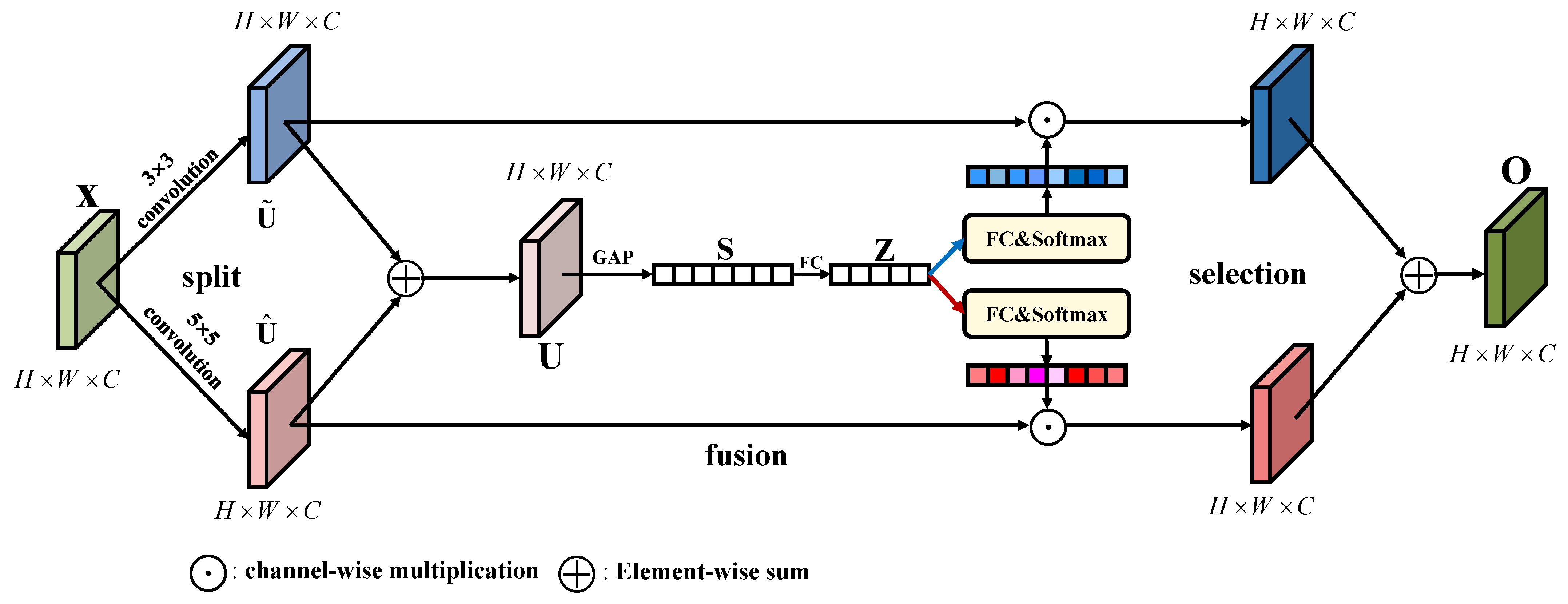
Figure 1 shows the illustration of the SK module, which is made up of three operations: split, fusion, and selection. The module utilizes feature maps $\mathit{X}\in {\mathbb{R}}^{H\times W\times C}$ as input and produces the output feature maps $\mathit{O}\in {\mathbb{R}}^{H\times W\times C}$. Therefore, the module can be presented as:

$$\mathit{O}=f_{\mathrm{sk}}(\mathit{X};\theta )$$

(4)

where $\theta$ denotes parameters in the module. H, W, and C are the height, width, and channel of feature maps. In the split operation, two transformations: $\mathit{X}\to \tilde{\mathit{U}}\in {\mathbb{R}}^{H\times W\times C}$ and $\mathit{X}\to \widehat{\mathit{U}}\in {\mathbb{R}}^{H\times W\times C}$ are utilized to illustrate, and 3 × 3 and 5 × 5 kernel sizes are used in the two transformations, respectively. Two output feature maps $\tilde{\mathit{U}}$ and $\widehat{\mathit{U}}$ can be formulated as:

$$\tilde{\mathit{U}}=\tilde{f}\left(\mathit{X}\right)=\mathit{X}\times {\mathit{W}}_{3\times 3}+\mathit{b}$$

(5)

$$\widehat{\mathit{U}}=\widehat{f}\left(\mathit{X}\right)=\mathit{X}\times {\mathit{W}}_{5\times 5}+\mathit{b}$$

(6)

where $\mathit{W}$ and $\mathit{b}$ are convolutional kernels and biases, respectively. Different kernel sizes are employed to extract multi-scale information. Moreover, the Batch Normalization (BN) and activation function are included in the two transformations.

In the SK module, the fusion operation aims to allow neurons to learn multi-scale features by automatically adjusting the kernel sizes jointly. Firstly, an element-wise summation combines feature maps from the split operation. The output $\mathit{U}\in {\mathbb{R}}^{H\times W\times C}$ is given by:

$$\mathit{U}=\tilde{\mathit{U}}\oplus \widehat{\mathit{U}}$$

(7)

where ⊕ represents element-wise addition operation. Then, a squeeze-and-excitation block (SE block) is utilized to extract the global information via global average pooling [45]. Finally, the output $\mathit{S}\in {\mathbb{R}}^C$ contains channel-wise statistics and is calculated by reducing $\mathit{U}$ through spatial dimensions using global average pooling (GAP):

$${\mathit{S}}_c=f_{GAP}\left({\mathit{U}}_c\right)=\frac{1}{H\times W}\sum _{i=1}^H\sum _{j=1}^W{\mathit{U}}_c(i,j)$$

(8)

where ${\mathit{S}}_c$ denotes the cth element of output $\mathit{S}$, and ${\mathit{U}}_c$ is the cth channel of the fusion feature map $\mathit{U}$. Then, a fully connected layer with a ReLU function is used to generate compact features that can guide precise and adaptive selections. The compact feature $\mathit{Z}\in {\mathbb{R}}^{\frac{C}{r}\times 1}$ can be formulated as:

$$\mathit{Z}=\mathrm{ReLU}(\mathit{W}·\mathit{S}),$$

(9)

where $\mathit{W}\in {\mathbb{R}}^{\frac{C}{r}\times C}$ is a weight matrix, and r denotes a reduction ratio. In this paper, the reduction ratio r is fixed at 16.

In the selection operation, selective kernel attention across channels is utilized to select different scales of features adaptively. The compact feature $\mathit{Z}$ is applied to compute the selective kernel attention vectors $\mathit{a}$ and $\mathit{b}$ by the fully connected layer and softmax function:

$${\mathit{a}}_c=\frac{e^{{\mathit{A}}_c\mathit{Z}}}{e^{{\mathit{A}}_c\mathit{Z}}+e^{{\mathit{B}}_c\mathit{Z}}}$$

(10)

$${\mathit{b}}_c=\frac{e^{{\mathit{B}}_c\mathit{Z}}}{e^{{\mathit{A}}_c\mathit{Z}}+e^{{\mathit{B}}_c\mathit{Z}}}$$

(11)

where ${\mathit{a}}_c$ and ${\mathit{b}}_c$ denote the cth element of attention vector $\mathit{a}$ and $\mathit{b}$. Here, $\mathit{A},\mathit{B}\in {\mathbb{R}}^{C\times \frac{C}{r}}$ and ${\mathit{A}}_c$ and ${\mathit{B}}_c$ are the cth row of $\mathit{A}$, $\mathit{B}$. Moreover, the elements ${\mathit{a}}_c$ and ${\mathit{b}}_c$ have the following relationship:

$${\mathit{a}}_c+{\mathit{b}}_c=1$$

(12)

Finally, the output feature map $\mathit{O}$ of the SK module with two kernel sizes is calculated by the attention vector as follows:

$$\mathit{O}=(\mathit{a}\otimes \tilde{\mathit{U}})\oplus (\mathit{b}\otimes \widehat{\mathit{U}})$$

(13)

Each neuron can modify the size of its receptive field using the SK module depending on multiple scales of input features. In the module, softmax attention is used to fuse different kernel sizes with the information in corresponding branches. Moreover, the module can capture target objects with multi-scales information, which is important for classification.

3.3. Self-Attention Module

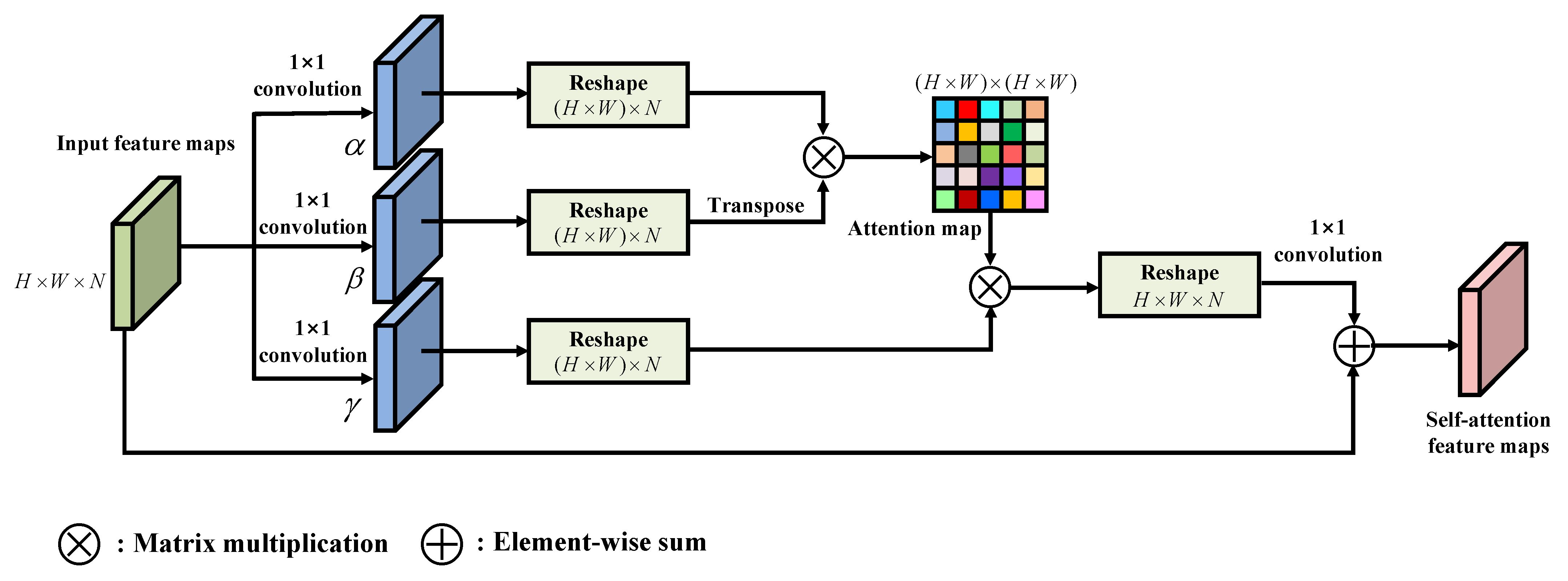
In order to capture more contextual and spatial information in the learning network, we use a self-attention module to build long-range dependency and extract the complex land cover areas effectively. The self-attention module is illustrated in Figure 2, where $\mathit{X}\in {\mathbb{R}}^{H\times W\times C}$ is the input feature map. H, W, and C denote the width, height, and channel, respectively. Then, three convolutions with $1\times 1$ kernel are employed to transform the input feature map into three diverse embeddings.

$$\begin{array}{cc}\hfill \alpha & ={\mathit{W}}_{\alpha }\left(\mathit{X}\right)\hfill \\ \hfill \beta & ={\mathit{W}}_{\beta }\left(\mathit{X}\right)\hfill \\ \hfill \gamma & ={\mathit{W}}_{\gamma }\left(\mathit{X}\right)\hfill \end{array}$$

(14)

where $\alpha \in {\mathbb{R}}^{H\times W\times N}$, $\beta \in {\mathbb{R}}^{H\times W\times N}$, $\gamma \in {\mathbb{R}}^{H\times W\times N}$, and N indicate the channel of reshaped feature map. Then, $\alpha$, $\beta$, and $\gamma$ are reshaped to $(H\times W)\times N$. To obtain the spatial self-attention map $\mathit{A}\in {\mathbb{R}}^{HW\times HW}$, the matrix multiplication is applied between $\alpha$ and the transpose of $\beta$ with the softmax function:

$${\mathit{A}}_{(i,j)}=\frac{exp\left({\alpha }_i\times {\beta }_j^T\right)}{{\sum }_{k=1}^{HW}exp\left({\alpha }_k\times {\beta }_j^T\right)}$$

(15)

Then, the spatial self-attention map $\mathit{A}$ is multiplied by $\gamma$, and the result is $\mathit{B}=\mathit{A}\times \gamma$.

The result $\mathit{B}$ is reshaped to $H\times W\times N$. The final self-attention enhanced feature map $\mathit{P}$ is formulated as:

$$\mathit{P}=F\left(\mathit{B}\right)+\mathit{X}$$

(16)

where $F(·)$ is the nolinear transformation implemented by a convolutional layer with $1\times 1$ kernel. It can be seen from Equation (16) that the attention feature map $\mathit{P}$ is the sum of the the global feature map and input feature map. The global feature map contains relationships across all positions in the PolSAR image. This property enables the network to build the global spatial dependency for pixels belonging to the same category. Moreover, the global information contained in the PolSAR image can significantly improve the robustness of deep neural networks when confronted with blur [46].

3.4. PolSAR Classification with HA-EDNet

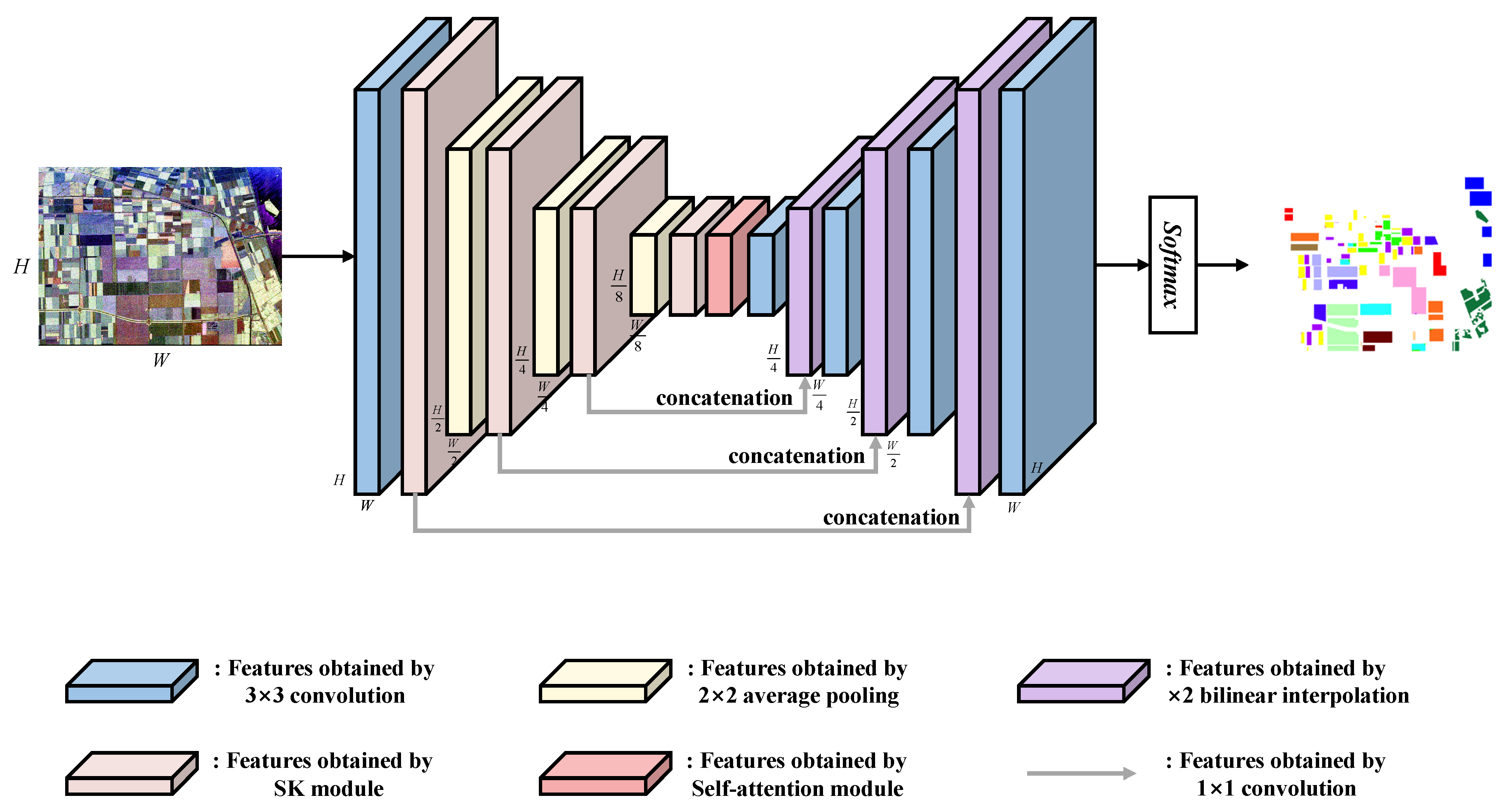
Patch-based CNN methods need to divide the input image into overlapping patches, which results in high computational complexity. This paper proposes a patch-free network architecture called HA-EDNet for full image classification. In patch-free networks, the explicit patching is replaced with the implicit receptive field of the model. The patch-free networks can avoid redundant computation on the overlapping areas and obtain a wider latent spatial context. The network accepts arbitrary-size images as input without pretreatment, and the output is the classification results of the whole image. The proposed model is described in the following.

As shown in Figure 3, the HA-EDNet is comprised of two basic subnetworks: (1) the encoder subnetwork and (2) the decoder subnetwork. As input, the coherence matrices of the whole PolSAR image are employed. Then, the encoder subnetwork is used to compute the hierarchical convolutional feature maps of the input PolSAR image, which is started with a 3 × 3 convolutional layer, a BN layer, and a ReLU function. The remaining part is composed of three SK modules and three downsampling layers. Here, 2 × 2 average pooling layers are utilized as the downsampling layers. In the top layer of the encoder subnetwork, the self-attention module is used to build long-range dependency. The decoder subnetwork is used to recover the spatial dimension of the coarsest convolutional feature map, which is a sample composed of three 3 × 3 convolutional layers and three upsample layers. Here, the upsampling layer is the bilinear interpolate function with a factor of 2. To effectively combine the spatial detail features in the encoder subnetwork and the semantic features in the decoder subnetwork, the feature maps of every SK module are added to the same size output of the decoder subnetwork. Finally, the softmax function is utilized to classify.

In the training process, the model is optimized by the cross-entropy loss function, which is written as:

$$\mathcal{L}=-\frac{1}{n}\sum _{i=1}^{n}y\times log\left(\sigma {\left(z\right)}_i\right)$$

(17)

$$y=\left\{\begin{array}{cc}1,\hfill & \mathrm{if}z\mathrm{belongs}\mathrm{to}\mathrm{class}i\hfill \\ 0,\hfill & \mathrm{otherwise}\hfill \end{array}\right.$$

(18)

where z is the predicted result of the network. When z belongs to the ith class, $y=1$; otherwise, $y=0$. $\sigma {\left(z\right)}_i$ is the output of the softmax function, which is the probability of belonging to a certain category.

4. Experiments and Results

In this part, we introduce four widely used PolSAR datasets employed in our experiments and experimental settings of the proposed approach. Additionally, classification results based on the proposed network and comparison approaches are presented.

4.1. Datasets

To evaluate the effectiveness of the proposed network, four PolSAR datasets are employed as follows:

(1)

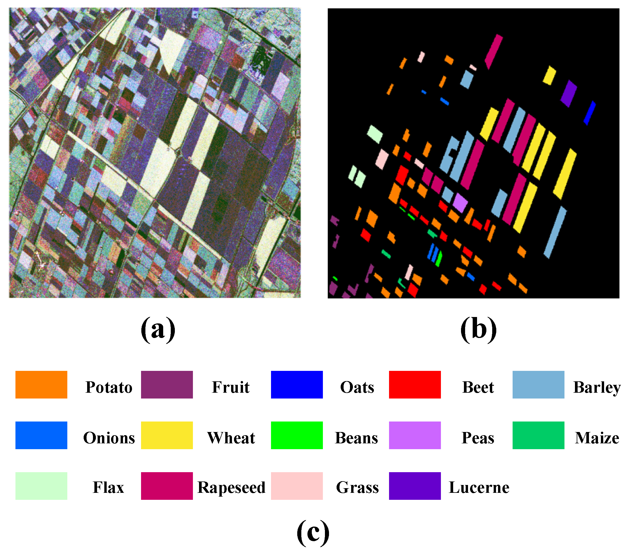
Flevoland-15 dataset: The Flevoland-15 dataset is the most widely used PolSAR dataset and is L-band polarimetric data obtained by the Airborne Synthetic Aperture Radar (AIRSAR) of Flevoland, Netherlands, in 1989. This dataset is regarded as a benchmark dataset for PolSAR classification. The pseudocolor image, ground truth, and legends of classes are shown in Figure 4.

(2)

Flevoland-14 dataset: The Flevoland-14 dataset is also L-band data collected by the AIRSAR in 1991 over Flevoland. The pseudocolor image, ground truth, and legends of classes are shown in Figure 5. This dataset includes fourteen types of objects.

(3)

Oberpfaffenhofen dataset: The Oberpfaffenhofen dataset is acquired from the L-band ESAR sensor that covers Oberpfaffenhofen, Germany. The pseudocolor image, ground truth, and legends of classes are shown in Figure 6. The ground truth contain three land cover types.

(4)

San Francisco dataset: The San Francisco dataset is obtained from the C-band RADARSAT-2, which covered San Francisco in 2008. The pseudocolor image, the ground truth, and legends of classes are shown in Figure 7. The ground truth of the dataset includes five types of objects.

4.2. Experimental Setting

In this paper, training samples adopt a randomly selected strategy from each class, while the remaining samples serve as the testing set. Three assessment measures, including overall accuracy (OA), average accuracy (AA), and the kappa coefficient (Kappa), are used to assess classification performance. The experiments of four datasets are implemented in Python 3.7 and Pytorch, with Intel Silver 4210v4 2.2GHz CPU, NVIDIA RTX 2080Ti GPU, and 64G RAM.

The input layer of the proposed approach has a size of $H\times W\times C$, where H and W are the height and width of the input, respectively. C denotes the channel of a PolSAR dataset, which is the nine-dimensional real vector. The initial weights are chosen randomly for all methods. Two improtant training parameters: learning rate and the number of iterations are set as 0.005 and 300, respectively. Every method is tested ten times using different training samples. The averaged results are employed to compare.

In the experiments, the training set is selected randomly from the ground truth. To solve the imbalance issue, we randomly choose labeled samples of each annotated class for the training set instead of dividing the labeled samples by an average percentage. Finally, the training and testing samples of four datasets are listed in

Table 1. Trainingand testing samples of the Flevoland-15 dataset.

Class Number	Region	Training Number	Testing Number	Total Number
1	Stem beam	100	6003	6103
2	Peas	100	9011	9111
3	Forest	100	14,844	14,944
4	Lucerne	100	9377	9477
5	Wheat 2	100	17,183	17,283
6	Beet	100	9950	10,050
7	Potato	100	15,192	15,292
8	Bare soil	100	2978	3078
9	Grass	100	6169	6269
10	Rapeseed	100	12,590	12,690
11	Barley	100	7059	7159
12	Wheat 1	100	10,491	10,591
13	Wheat 3	100	21,200	21,300
14	Water	100	13,376	13,476
15	Building	100	376	476
Total		1500	155,799	157,299

,

Table 2. Training and testing samples of the Flevoland-14 dataset.

Class Number	Region	Training Number	Testing Number	Total Number
1	Potato	100	21,513	21,613
2	Fruit	100	4252	4352
3	Oats	100	1294	1394
4	Beet	100	10,717	10,817
5	Barley	100	24,443	24,543
6	Onions	100	2030	2130
7	Wheat	100	26,177	26,277
8	Beans	100	982	1082
9	Peas	100	2060	2160
10	Maize	100	1190	1290
11	Flax	100	4201	4301
12	Rapeseed	100	28,135	28,235
13	Grass	100	4104	4204
14	Lucerne	100	2852	2952
Total		1400	133,950	135,350

,

Table 3. Training and testing samples of the Oberpfaffenhofen dataset.

Class Number	Region	Training Number	Testing Number	Total Number
1	Built-up	100	327,951	328,051
2	Wood land	100	246,573	246,673
3	Open areas	100	736,794	736,894
Total		300	1,311,318	1,311,618

and

Table 4. Training and testing samples of the San Francisco dataset.

Class Number	Region	Training Number	Testing Number	Total Number
1	Water	100	689,707	689,807
2	Vegetation	100	198,502	198,602
3	High-Density Urban	100	112,161	112,261
4	Low-Density Urban	100	275,576	275,674
5	Developed	100	65,473	65,573
Total		500	1,497,218	1,497,718

.

4.3. Result on the Flevoland-15 Dataset

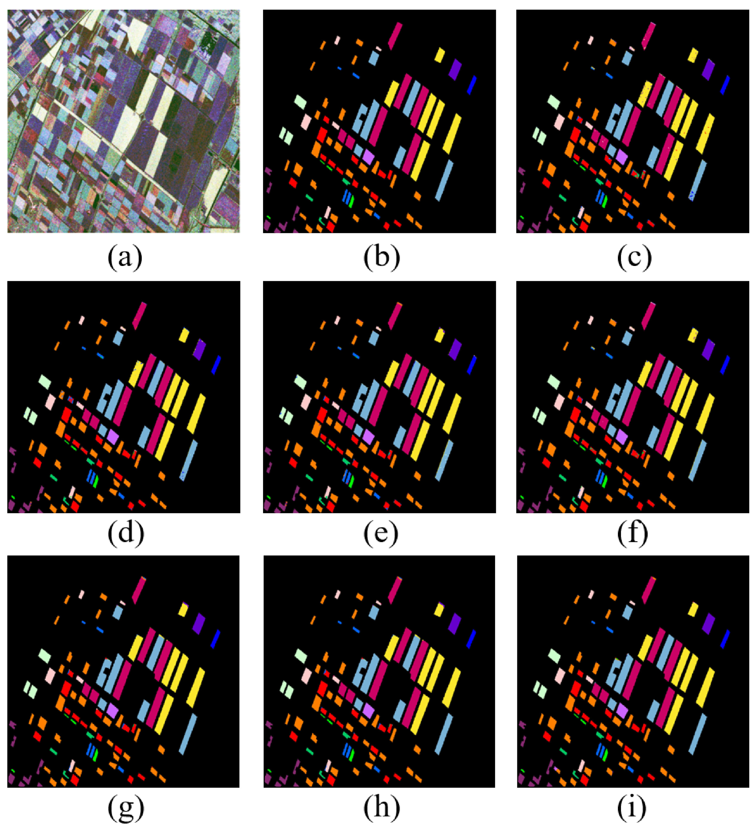
The first dataset in Flevoland is employed to evaluate the efficiency of the proposed HA-EDNet method. Several state-of-the-art models are chosen for comparison, including CNN, 3D-CNN [47], multi-scale CNN (MS-CNN) [48], complex-valued CNN (CV-CNN) [49], FCN [50], and U-Net [51]. The classification accuracies of seven different approaches are shown in

Table 5. Classification results of different methods in the Flevoland-15 dataset.

Region	CNN	3D-CNN	MS-CNN	CV-CNN	FCN	U-Net	Proposed
Stem beam	68.02	69.21	74.06	98.48	95.45	97.90	99.35
Peas	96.81	96.66	96.44	97.50	99.73	99.89	99.89
Forest	96.24	95.51	99.32	92.09	99.83	98.90	99.73
Lucerne	97.29	97.11	96.09	96.63	95.81	92.96	97.61
Wheat 2	87.66	87.60	83.99	93.39	99.01	98.10	99.58
Beet	98.77	93.73	97.78	96.62	99.57	98.14	99.78
Potato	91.62	95.16	96.29	95.35	99.67	98.18	99.26
Bare soil	99.57	100	99.80	99.83	100	100	100
Grass	86.82	86.19	89.48	90.14	99.82	99.47	99.92
Rapeseed	88.82	89.72	93.70	78.05	66.57	64.83	98.19
Barley	99.17	97.93	99.68	95.01	99.86	99.97	100
Wheat 1	92.57	92.54	94.26	80.81	96.81	95.83	99.98
Wheat 3	98.47	98.45	99.08	95.52	99.93	99.82	99.04
Water	71.52	87.06	78.24	98.85	92.80	84.29	100
Building	56.69	98.94	71.55	98.67	100	97.61	100
OA	91.05	92.48	92.82	93.05	95.81	94.35	99.39
AA	88.67	92.39	91.32	93.80	96.32	95.06	99.49
Kappa	0.9024	0.9180	0.9217	0.9241	0.9543	0.9384	0.9933

. For the PolSAR classification task, the visual performance of the classification network is essential. Figure 8 shows the classification results of the Flevoland-15 dataset. The pseudocolor image, ground truth map, CNN, 3D-CNN, MS-CNN, CV-CNN, FCN, U-Net, and HA-EDNet classification map are shown in Figure 8a–i, respectively. Consequently, several conclusions can be achieved from Figure 8 and Table 5. As is shown in Figure 8c,e, the MS-CNN classifier has a better performance than the CNN classifier because the MS-CNN classifier can extract multi-scale features that are strongly discriminative. HA-EDNet methods are superior to the FCN and U-Net classifier in spatial uniformity when comparing Figure 8g–i. It can be attributed to the fusion of spatial detail features, and the introduction of the hybrid attention mechanism can capture more discriminative features. In addition, the proposed HA-EDNet approach produces classification results with less noise and more precision than prior methods. Table 5 lists the results of the seven methods. From Table 5, we can find that the MS-CNN method wins nine categories and achieves higher accuracies (OA of 92.82%, AA of 91.32%, and Kappa of 0.9217) than CNN. It indicates that using multi-scale features improve the classification accuracy. Comparing the results of patch-wise with patch-free methods, patch-free methods obtain more accurate results than patch-based methods. It demonstrates that patch-free models can effectively extract spatial features. From Table 5, it is shown that the proposed HA-EDNet method obtained a higher OA of 99.39%, exceeding CNN by about 8.3%. These results demonstrate the effectiveness of the proposed module. In

Table 6. Classification of state-of-the-art methods on the Flevoland-15 dataset.

Method	Training Ratio	Class Number	OA
N-cluster GAN [52]	5%	15	99.10%
PolMPCNN [53]	1%	15	99.14%
HCapsNet [54]	1%	15	99.04%
AMSE-LSTM [34]	1%	15	97.09%
Proposed method	<1%	15	99.39%

, we also compare the proposed method with the other four state-of-the-art methods, and the results are shown in Table 6. The proposed method achieves the highest accuracy with less than 1% training samples.

4.4. Result on the Flevoland-14 Dataset

In the experiment on the Flevoland-14 dataset,

Table 7. Classification results of different methods in the Flevoland-14 dataset.

Region	CNN	3D-CNN	MS-CNN	CV-CNN	FCN	U-Net	Proposed
Potato	99.54	99.23	99.39	99.29	99.83	99.87	98.56
Fruit	99.69	98.89	98.68	99.98	100	100	100
Oats	99.07	99.23	98.30	99.31	100	100	100
Beet	91.44	94.67	95.98	95.24	90.33	91.28	99.73
Barley	98.02	98.14	96.96	98.72	99.74	99.79	99.28
Onions	92.22	94.78	91.23	93.15	98.28	97.54	99.80
Wheat	98.33	98.50	99.19	98.94	99.78	99.79	99.81
Beans	98.68	98.47	98.57	99.08	95.51	97.66	98.98
Peas	99.32	99.81	99.95	100	100	100	99.95
Maize	97.31	96.05	96.64	99.16	98.99	99.92	100
Flax	99.57	99.38	97.24	99.91	100	100	100
Rapeseed	98.43	99.03	99.07	99.02	99.23	99.27	99.48
Grass	96.17	96.98	95.57	97.47	96.66	97.95	100
Lucerne	96.84	95.16	98.88	96.84	99.76	99.86	100
OA	97.84	98.23	98.19	98.59	98.77	98.93	99.46
AA	97.47	97.74	97.55	98.29	98.44	98.78	99.69
Kappa	0.9746	0.9791	0.9787	0.9833	0.9855	0.9873	0.9936

provides the comparisons of OA, AA, Kappa, and the accuracy of each terrain. As shown in Table 7, the classification results of the HA-EDNet method are superior to those of the other comparison methods. The OA value of the proposed method is about 1.62%, 1.23%, 1.27%, 0.87%, 0.69%, and 0.53% higher than other methods. The proposed method achieves the highest accuracies in ten areas and achieved 100% accuracies in six areas. Figure 9 presents the classification maps for each approach. Figure 9c–f gives the classification results of CNN, 3D-CNN, MS-CNN, and CV-CNN, respectively. It is clear that the discrete misclassifications of patch-wise methods exist. Figure 9g,f show the classification results of FCN and U-Net. It can be seen that patch-free methods have better uniformity than patch-wise methods. However, they still have some misclassification in border regions. The classification map for the proposed method is shown in Figure 9i. We can notice that the proposed HA-attention has the best uniformity and performs better in border regions. The primary reason is the extraction capacity of multi-scale features and contextual information by the SK module and self-attention. In conclusion, the classification results can demonstrate the efficacy of the HA-attention model.

4.5. Result on the Oberpfaffenhofen Dataset

Table 8. Classification results of different methods in the Oberpfaffenhofen dataset.

Region	CNN	3D-CNN	MS-CNN	CV-CNN	FCN	U-Net	Proposed
Built-up areas	86.23	85.49	86.56	79.12	90.89	92.87	93.99
Wood land	45.07	52.32	56.30	94.31	97.65	97.95	98.82
Open areas	92.77	93.31	92.50	92.40	92.61	94.57	96.97
OA	82.17	83.65	84.21	89.44	93.13	94.78	96.57
AA	74.69	77.04	78.45	88.61	93.72	95.13	96.59
Kappa	0.6937	0.7191	0.7300	0.8225	0.8847	0.9120	0.9418

shows the classification results of each model for three terrain classes in the Oberpfaffenhofen dataset. It can be seen from Table 8 that the performance of the proposed approach is superior to other comparison methods. The OA value of the proposed approach is 14.4%, 12.92%, 12.36%, 7.13%, 4.44%, and 1.79% higher than other comparison methods. It is obvious that patch-wise methods have poor performance. The Kappa coefficients of the patch-wise methods are no more than 0.83. It indicates that these methods do not have good consistency. The patch-free methods perform better in the dataset. The OA values of FCN and U-Net are over 90%. Moreover, the consistency is enhanced due to the spatial information. The proposed method makes further improvements compared to FCN and v. The HA-attention method presents an appealing classification performance, attaining a 96.57% OA value, a 96.59% AA value, and a Kappa coefficient of 0.9418. The experimental results demonstrate that the overall performance of the proposed approach is better than other comparison approaches. Figure 10 depicts classification maps of each method. It can be seen that CNN, 3D-CNN, MS-CNN, and CV-CNN have poor accuracies and present more misclassifications. The FCN and U-Net classifications have been improved, although border areas still include several misclassifications. Compared with the other approaches, the visual performance of the proposed approaches on each land cover area shows a better consistency. In addition, the border regions of the proposed approach on the classification map are much more uniform than those of existing comparison approaches.

4.6. Result on the San Francisco Dataset

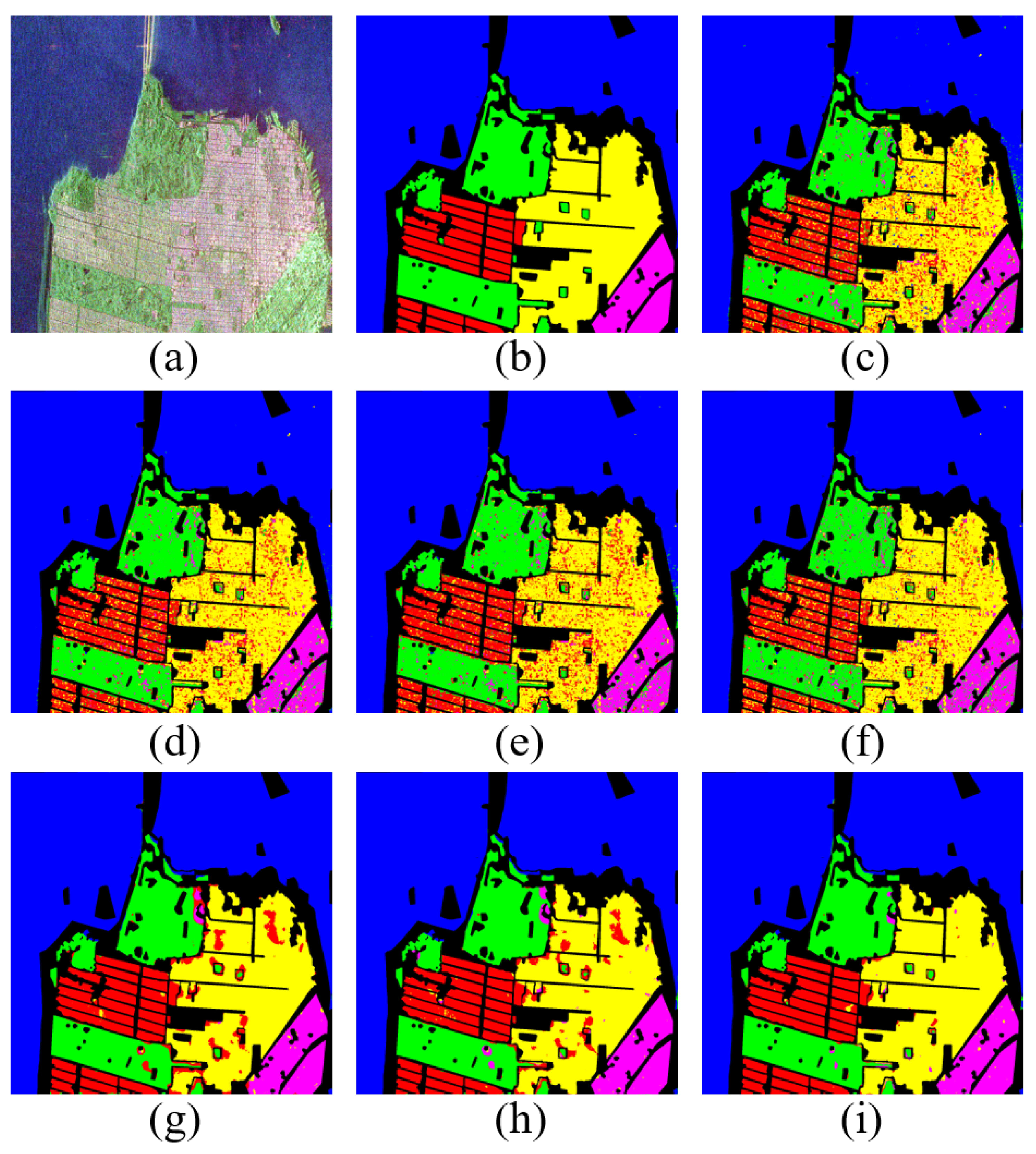
In order to evaluate the effectivity of the HA-EDNet approach, we also performed experiments on the RADARSAT-2 San Francisco dataset. The dataset has 1300 × 1300 pixels, and the ground truth comprises five classes. The classification results of various approaches on the San Francisco dataset are shown in

Table 9. Classification results of different methods in the San Francisco dataset.

Region	CNN	3D-CNN	MS-CNN	CV-CNN	FCN	U-Net	Proposed
Water	99.53	99.87	99.82	99.97	99.99	99.97	99.93
Vegetation	88.32	88.81	89.13	86.69	95.36	96.63	95.53
High-Density Urban	79.16	79.80	85.25	78.59	94.78	96.94	99.21
Low-Density Urban	81.12	82.55	79.71	85.13	83.80	85.82	98.47
Developed	84.22	86.82	86.89	85.38	95.91	95.39	98.55
OA	91.64	92.36	92.26	92.45	95.35	96.10	98.85
AA	86.47	87.57	88.16	87.15	93.97	94.95	98.34
Kappa	0.8744	0.8851	0.8838	0.8862	0.9302	0.9413	0.9827

. From Table 9, the results show that the proposed approach obtains the optimal classification performance. The OA of the proposed network is 7.21%, 6.49%, 6.59%, 6.4%, 3.5%, and 2.75% higher than CNN, 3D-CNN, MS-CNN, CV-CNN, FCN, and U-Net, respectively. The proposed approach reaches a classification of 98.85% OA, 98.34% AA, and a Kappa coefficient of 0.9827. The classification maps of each model are shown in Figure 11. It is obvious that the classification results of CNN, 3D-CNN, MS-CNN, and CV-CNN models are poor, with more noise and speckles. The classification results of the FCN and U-Net model have less noise, which improves the classification performance of these models. The proposed model achieves significant performance gains with a combination of the hybrid attention blocks. The results demonstrate the effectiveness of the HA-EDNet approach.

5. Analysis and Discussion

5.1. Ablation Study

In this part, we evaluate how the classification performance is affected by each module of the proposed method. The effectiveness of different modules are presented in

Table 10. Performance contribution of each module in HA-EDNet.

Method	Based Method	+SK	+SA	+SA+SK
Patch-free model	✓	✓	✓	✓
Selective kernel attention (SK)		✓		✓
Self-attention (SA)			✓	✓
Flevoland-15	96.27	98.66	98.89	99.39
Flevoland-14	98.76	99.25	98.96	99.46
Oberpfaffenhofen	95.61	95.81	96.26	96.57
San Francisco	97.44	98.46	98.30	98.85

. From Table 10, the results indicate that both selective kernel attention and self-attention can significantly improve classification performance. It can be seen that the selective kernel attention increases the OA values by 2.39%, 0.49%, 0.2%, and 1.02% for four datasets, owing to its capability of attention-based multi-scale feature extraction. The attention-based multi-scale features can highlight and combine different scale information in the network. The self-attention module increases the OA values by 2.72%, 0.2%, 0.65%, and 0.86%, respectively. It is useful for exploring long-range dependency over local spatial features. Combining the SK module and self-attention module for all four datasets can achieve the best OA values.

5.2. Effect of Training Samples

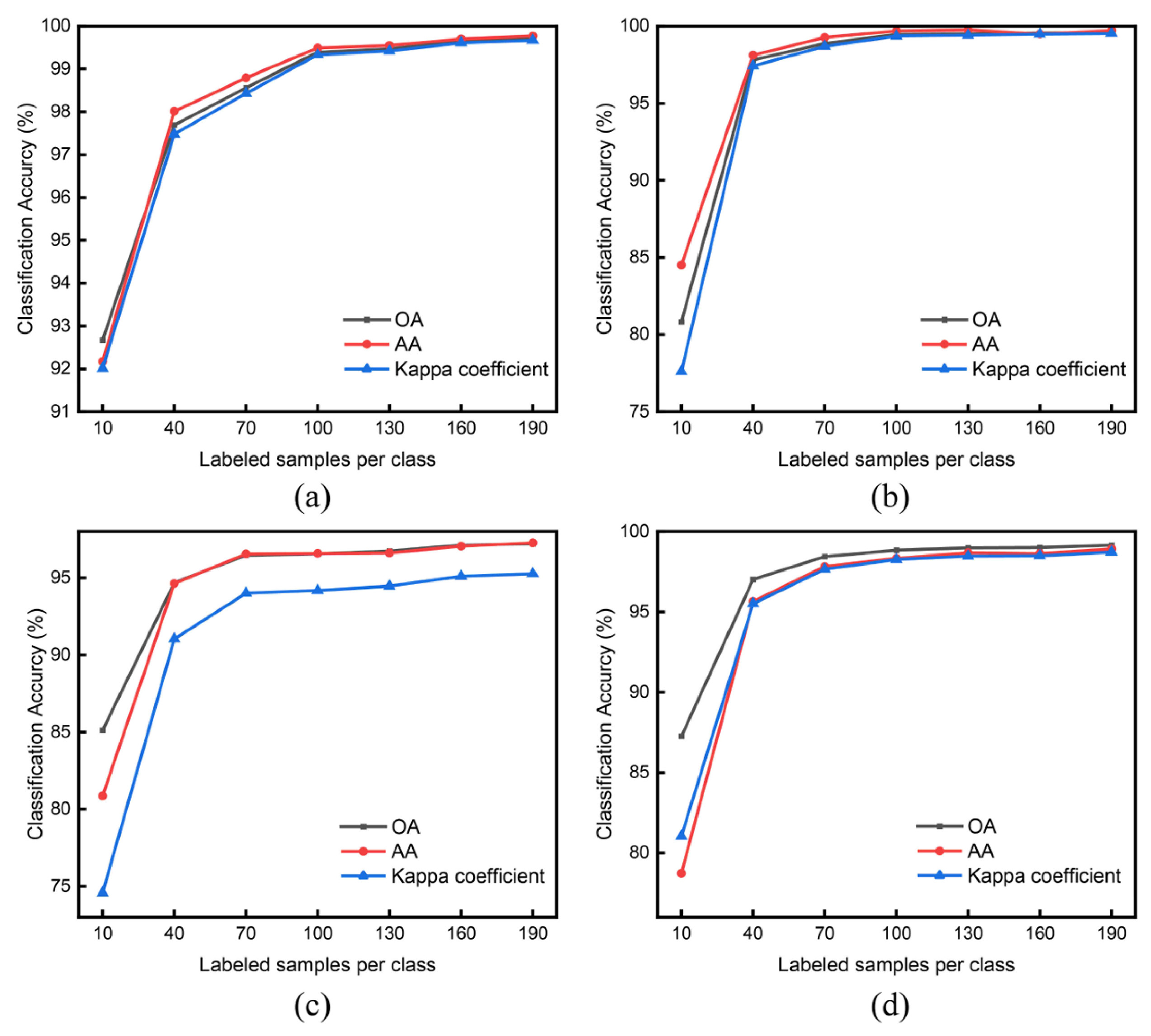
The experimental results have demonstrated that the HA-EDNet network achieves excellent performance for PolSAR image classification, especially in cases of fewer training samples. In this part, we would like to further explore the scenarios of extremely rare training samples. The results of OA, AA, and Kappa with respect to a changed number of training samples are shown in Figure 12. For four datasets, training samples of per class are varied from 10 to 190 with an interval of 30. As expected, the classification accuracies increase with the training number increasing. It is obvious that the proposed approach performs well (up to 80%) when it only has 10 training samples of per class. Therefore, the proposed approach is suitable in the environment when training samples are rare.

5.3. Effect of Different Kernels

In the proposed method, the main parameter that affects the model performance is the kernel number of SK modules. The kernel size determines the range of the receptive field that is used to extract features. We verify the model performance when the kernel groups are (1, 3), (3, 5), (5, 7), (1, 3, 5), (3, 5, 7), and (1, 3, 5, 7). In

Table 11. Performance contribution of different kernels in the SK module.

Kernel Number	(1, 3)	(3, 5)	(5, 7)	(1, 3, 5)	(3, 5, 7)	(1, 3, 5, 7)
Flevoland-15	98.24	99.39	99.31	98.89	99.26	99.22
Flevoland-14	98.01	99.46	99.39	99.18	99.36	99.33
Oberpfaffenhofen	96.02	96.57	96.22	96.16	96.08	95.89
San Francisco	98.48	98.85	98.51	98.73	98.81	98.69

and Figure 13, the classification results show that using 3 × 3, 5 × 5, and 7 × 7 kernels can achieve better classification performance. When the kernel group is (3, 5), the model obtains the best classification accuracies. It demonstrates that 3 × 3 and 5 × 5 kernel groups are beneficial for capturing multi-scale features and significantly improve the classification performance.

6. Conclusions

A novel encoder–decoder method is proposed to extract multi-scale features and long-range dependency based on a hybrid attention mechanism for PolSAR classification in this paper. Inspired by the way humans mimic cognitive attention, the network devotes more focus to the small but important parts of the data, known as the attention mechanism. This mechanism is incorporated into our model. In this method, the patch-free framework, SK module, and self-attention module are utilized. First, an encoder–decoder network is built for patch-free classification, allowing an entire PolSAR image as input and not requiring dividing the image into overlapping patches. Then, the SK module is embedded into the EDNet, which can capture multi-scale features by automatically adjusting the kernel size. Finally, self-attention is employed to extract long-range dependency, which can improve classification performance. In the experiments, four PolSAR datasets are employed to test the effectiveness of the HA-EDNet architecture. The experimental results show that the proposed approach has effective and superior performance compared with some state-of-the-art approaches.

Other attention mechanisms will be introduced into the model for better feature extraction performance in future work. Moreover, a more effective patch-free model will also be investigated in our future works.

References

1. Duan, D.; Wang, Y. Reflection of and vision for the decomposition algorithm development and application in earth observation studies using PolSAR technique and data. Remote Sens. Environ. 2021, 261, 112498. [Google Scholar] [CrossRef]
2. Zhai, W.; Zhang, J.; Xiao, X.; Wang, J.; Zhang, H.; Yin, X.; Wu, Z. Damaged building extraction from post-earthquake PolSAR data based on the Fourier transform. Remote Sens. Lett. 2021, 12, 594–603. [Google Scholar] [CrossRef]
3. Parrella, G.; Hajnsek, I.; Papathanassiou, K. Model-Based Interpretation of PolSAR Data for the Characterization of Glacier Zones in Greenland. IEEE J. Sel. Top. Appl. Earth Obs. Remote Sens. 2021, 14, 11593–11607. [Google Scholar] [CrossRef]
4. Mahdavi, S.; Salehi, B.; Huang, W.; Amani, M.; Brisco, B. A PolSAR Change Detection Index Based on Neighborhood Information for Flood Mapping. Remote Sens. 2019, 11, 1854. [Google Scholar] [CrossRef] [Green Version]
5. Fan, J.; Zhao, J.; An, W.; Hu, Y. Marine Floating Raft Aquaculture Detection of GF-3 PolSAR Images Based on Collective Multikernel Fuzzy Clustering. IEEE J. Sel. Top. Appl. Earth Obs. Remote Sens. 2019, 12, 2741–2754. [Google Scholar] [CrossRef]
6. Zhai, W.; Shen, H.; Huang, C.; Pei, W. Fusion of Polarimetric and Texture Information for Urban Building Extraction from Fully Polarimetric SAR Imagery. Remote Sens. Lett. 2016, 7, 31–40. [Google Scholar] [CrossRef]
7. Han, P.; Han, B.; Shi, Q.; Song, T.; Lu, X.; Zhang, Z. Aircraft Detection Based on Eigen Decomposition and Scattering Similarity for PolSAR Image. In Proceedings of the 2018 IEEE/AIAA 37th Digital Avionics Systems Conference (DASC), London, UK, 23–27 September 2018; pp. 1–6. [Google Scholar] [CrossRef]
8. Wang, H.; Xing, C.; Yin, J.; Yang, J. Land Cover Classification for Polarimetric SAR Images Based on Vision Transformer. Remote Sens. 2022, 14, 4656. [Google Scholar] [CrossRef]
9. Cloude, S.R.; Pottier, E. A Review of Target Decomposition Theorems in Radar Polarimetry. IEEE Trans. Geosci. Remote Sens. 1996, 34, 498–518. [Google Scholar] [CrossRef]
10. Chiang, C.Y.; Chen, K.S.; Chu, C.Y.; Chang, Y.L.; Fan, K.C. Color Enhancement for Four-Component Decomposed Polarimetric SAR Image Based on a CIE-Lab Encoding. Remote Sens. 2018, 10, 545. [Google Scholar] [CrossRef]
11. Krogager, E. New Decomposition of the Radar Target Scattering Matrix. Electron. Lett. 1990, 18, 1525–1527. [Google Scholar] [CrossRef]
12. Lee, J.S.; Schuler, D.L.; Ainsworth, T.L. Polarimetric SAR Data Compensation for Terrain Azimuth Slope Variation. IEEE Trans. Geosci. Remote Sens. 2000, 38, 2153–2163. [Google Scholar] [CrossRef]
13. Cameron, W.L.; Rais, H. Conservative Polarimetric Scatterers and Their Role in Incorrect Extensions of the Cameron Decomposition. IEEE Trans. Geosci. Remote Sens. 2006, 44, 3506–3516. [Google Scholar] [CrossRef]
14. Ballester-Berman, J.D.; Lopez-Sanchez, J.M. Applying the Freeman–Durden Decomposition Concept to Polarimetric SAR Interferometry. IEEE Trans. Geosci. Remote Sens. 2009, 48, 466–479. [Google Scholar] [CrossRef]
15. Guo, S.; Tian, Y.; Li, Y.; Chen, S.; Hong, W. Unsupervised Classification Based on H/alpha Decomposition and Wishart Classifier for Compact Polarimetric SAR. In Proceedings of the 2015 IEEE International Geoscience and Remote Sensing Symposium (IGARSS), Milan, Italy, 26–31 July 2015; pp. 1614–1617. [Google Scholar] [CrossRef]
16. Erith, M.; Alfonso, Z.; Erik, L. A Multi-Sensor Approach to Separate Palm Oil Plantations from Forest Cover Using NDFI and a Modified Pauli Decomposition Technique. In Proceedings of the IGARSS 2020-2020 IEEE International Geoscience and Remote Sensing Symposium, Waikoloa, HI, USA, 26 September–2 October 2020; pp. 4481–4484. [Google Scholar] [CrossRef]
17. Lee, J.S.; Grunes, M.R.; Ainsworth, T.L.; Du, L.J.; Schuler, D.L.; Cloude, S.R. Unsupervised Classification Using Polarimetric Decomposition and the Complex Wishart Classifier. IEEE Trans. Geosci. Remote Sens. 1999, 37, 2249–2258. [Google Scholar] [CrossRef]
18. Liu, F.; Jiao, L.; Hou, B.; Yang, S. POL-SAR Image Classification Based on Wishart DBN and Local Spatial Information. IEEE Trans. Geosci. Remote Sens. 2016, 54, 3292–3308. [Google Scholar] [CrossRef]
19. Jiao, L.; Liu, F. Wishart Deep Stacking Network for Fast POLSAR Image Classification. IEEE Trans. Image Process. 2016, 25, 3273–3286. [Google Scholar] [CrossRef]
20. Xie, W.; Jiao, L.; Hou, B.; Ma, W.; Zhao, J.; Zhang, S.; Liu, F. POLSAR Image Classification via Wishart-AE Model or Wishart-CAE Model. IEEE J. Sel. Top. Appl. Earth Obs. Remote Sens. 2017, 10, 3604–3615. [Google Scholar] [CrossRef]
21. Okwuashi, O.; Ndehedehe, C.E.; Olayinka, D.N.; Eyoh, A.; Attai, H. Deep Support Vector Machine for PolSAR Image Classification. Int. J. Remote Sens. 2021, 42, 6498–6536. [Google Scholar] [CrossRef]
22. Yin, Q.; Cheng, J.; Zhang, F.; Zhou, Y.; Shao, L.; Hong, W. Interpretable POLSAR Image Classification Based on Adaptive-Dimension Feature Space Decision Tree. IEEE Access 2020, 8, 173826–173837. [Google Scholar] [CrossRef]
23. Richardson, A.; Goodenough, D.G.; Chen, H.; Moa, B.; Hobart, G.; Myrvold, W. Unsupervised Nonparametric Classification of Polarimetric SAR Data Using the K-nearest Neighbor Graph. In Proceedings of the 2010 IEEE International Geoscience and Remote Sensing Symposium, Honolulu, HI, USA, 25–30 July 2010; pp. 1867–1870. [Google Scholar] [CrossRef]
24. Otter, D.W.; Medina, J.R.; Kalita, J.K. A Survey of the Usages of Deep Learning for Natural Language Processing. IEEE Trans. Neural Netw. Learn. Syst. 2020, 32, 604–624. [Google Scholar] [CrossRef] [Green Version]
25. Ouhami, M.; Hafiane, A.; Es-Saady, Y.; El Hajji, M.; Canals, R. Computer Vision, IoT and Data Fusion for Crop Disease Detection Using Machine Learning: A Survey and Ongoing Research. Remote Sens. 2021, 13, 2486. [Google Scholar] [CrossRef]
26. Wu, W.; Li, H.; Li, X.; Guo, H.; Zhang, L. PolSAR Image Semantic Segmentation Based on Deep Transfer Learning—Realizing Smooth Classification With Small Training Sets. IEEE Geosci. Remote Sens. Lett. 2019, 16, 977–981. [Google Scholar] [CrossRef]
27. Nie, W.; Huang, K.; Yang, J.; Li, P. A Deep Reinforcement Learning-Based Framework for PolSAR Imagery Classification. IEEE Trans. Geosci. Remote Sens. 2021, 60, 1–15. [Google Scholar] [CrossRef]
28. Zhang, L.; Ma, W.; Zhang, D. Stacked Sparse Autoencoder in PolSAR Data Classification Using Local Spatial Information. IEEE Geosci. Remote Sens. Lett. 2016, 13, 1359–1363. [Google Scholar] [CrossRef]
29. Zhou, Y.; Wang, H.; Xu, F.; Jin, Y.Q. Polarimetric SAR Image Classification Using Deep Convolutional Neural Networks. IEEE Geosci. Remote Sens. Lett. 2016, 13, 1935–1939. [Google Scholar] [CrossRef]
30. Wang, L.; Xu, X.; Dong, H.; Gui, R.; Yang, R.; Pu, F. Exploring Convolutional LSTM for PolSAR Image Classification. In Proceedings of the IGARSS 2018-2018 IEEE International Geoscience and Remote Sensing Symposium, Valencia, Spain, 22–27 July 2018; pp. 8452–8455. [Google Scholar] [CrossRef]
31. Zheng, Z.; Zhong, Y.; Ma, A.; Zhang, L. FPGA: Fast Patch-Free Global Learning Framework for Fully End-to-End Hyperspectral Image Classification. IEEE Trans. Geosci. Remote Sens. 2020, 58, 5612–5626. [Google Scholar] [CrossRef]
32. Chen, Z.; Tong, L.; Qian, B.; Yu, J.; Xiao, C. Self-Attention-Based Conditional Variational Auto-Encoder Generative Adversarial Networks for Hyperspectral Classification. Remote Sens. 2021, 13, 3316. [Google Scholar] [CrossRef]
33. Dong, H.; Zhang, L.; Lu, D.; Zou, B. Attention-Based Polarimetric Feature Selection Convolutional Network for PolSAR Image Classification. IEEE Geosci. Remote Sens. Lett. 2022, 19, 1–5. [Google Scholar] [CrossRef]
34. Hua, W.; Wang, X.; Zhang, C.; Jin, X. Attention-Based Multiscale Sequential Network for PolSAR Image Classification. IEEE Geosci. Remote Sens. Lett. 2022, 19, 1–5. [Google Scholar] [CrossRef]
35. Yang, Z.; Zhang, Q.; Chen, W.; Chen, C. PolSAR Image Classification Based on Resblock Combined with Attention Model. In Proceedings of the 2021 IEEE 6th International Conference on Signal and Image Processing (ICSIP), Nanjing, China, 22–24 October 2021; pp. 340–344. [Google Scholar] [CrossRef]
36. Ren, S.; Zhou, F. Polsar Image Classification with Complex-Valued Residual Attention Enhanced U-NET. In Proceedings of the 2021 IEEE International Geoscience and Remote Sensing Symposium IGARSS, Brussels, Belgium, 11–16 July 2021; pp. 3045–3048. [Google Scholar] [CrossRef]
37. Yang, B.; Wang, L.; Wong, D.F.; Shi, S.; Tu, Z. Context-Aware Self-Attention Networks for Natural Language Processing. Neurocomputing 2021, 458, 157–169. [Google Scholar] [CrossRef]
38. Gao, W.; Zhang, L.; Huang, W.; Min, F.; He, J.; Song, A. Deep Neural Networks for Sensor-Based Human Activity Recognition Using Selective Kernel Convolution. IEEE Trans. Instrum. Meas. 2021, 70, 1–13. [Google Scholar] [CrossRef]
39. Long, J.; Shelhamer, E.; Darrell, T. Fully Convolutional Networks for Semantic Segmentation. In Proceedings of the IEEE Conference on Computer Vision and Pattern Recognition, Boston, MA, USA, 7–12 June 2015; pp. 3431–3440. [Google Scholar]
40. Xu, R.; Tao, Y.; Lu, Z.; Zhong, Y. Attention-Mechanism-Containing Neural Networks for High-Resolution Remote Sensing Image Classification. Remote Sens. 2018, 10, 1602. [Google Scholar] [CrossRef] [Green Version]
41. Ghaffarian, S.; Valente, J.; van der Voort, M.; Tekinerdogan, B. Effect of Attention Mechanism in Deep Learning-Based Remote Sensing Image Processing: A Systematic Literature Review. Remote Sens. 2021, 13, 2965. [Google Scholar] [CrossRef]
42. Shaw, P.; Uszkoreit, J.; Vaswani, A. Self-Attention with Relative Position Representations. arXiv 2018, arXiv:1803.02155. [Google Scholar] [CrossRef]
43. Zhao, H.; Jia, J.; Koltun, V. Exploring Self-Attention for Image Recognition. In Proceedings of the IEEE/CVF Conference on Computer Vision and Pattern Recognition, Seattle, WA, USA, 13–19 June 2020; pp. 10076–10085. [Google Scholar] [CrossRef]
44. Li, X.; Wang, W.; Hu, X.; Yang, J. Selective kernel networks. In Proceedings of the IEEE/CVF Conference on Computer Vision and Pattern Recognition, Long Beach, CA, USA, 15–20 June 2019; pp. 510–519. [Google Scholar]
45. Hu, J.; Shen, L.; Sun, G. Squeeze-and-excitation networks. In Proceedings of the IEEE Conference on Computer Vision and Pattern Recognition, Salt Lake City, UT, USA, 18–23 June 2018; pp. 7132–7141. [Google Scholar]
46. Pu, W.; Bao, Y. RPCA-AENet: Clutter Suppression and Simultaneous Stationary Scene and Moving Targets Imaging in the Presence of Motion Errors. IEEE Trans. Neural Networks Learn. Syst. 2022, 1–14. [Google Scholar] [CrossRef]
47. Zhang, L.; Chen, Z.; Zou, B.; Gao, Y. Polarimetric SAR Terrain Classification Using 3D Convolutional Neural Network. In Proceedings of the IGARSS 2018-2018 IEEE International Geoscience and Remote Sensing Symposium, Valencia, Spain, 22–27 July 2018; pp. 4551–4554. [Google Scholar] [CrossRef]
48. Gong, Z.; Zhong, P.; Yu, Y.; Hu, W.; Li, S. A CNN with Multiscale Convolution and Diversified Metric for Hyperspectral Image Classification. IEEE Trans. Geosci. Remote Sens. 2019, 57, 3599–3618. [Google Scholar] [CrossRef]
49. Zhang, Z.; Wang, H.; Xu, F.; Jin, Y.Q. Complex-valued Convolutional Neural Network and Its Application in Polarimetric SAR Image Classification. IEEE Trans. Geosci. Remote Sens. 2017, 55, 7177–7188. [Google Scholar] [CrossRef]
50. Liu, X.; Jiao, L.; Tang, X.; Sun, Q.; Zhang, D. Polarimetric Convolutional Network for PolSAR Image Classification. IEEE Trans. Geosci. Remote Sens. 2018, 57, 3040–3054. [Google Scholar] [CrossRef] [Green Version]
51. Ronneberger, O.; Fischer, P.; Brox, T. U-net: Convolutional Networks for Biomedical Image Segmentation. In Proceedings of the International Conference on Medical Image Computing and Computer-Assisted Intervention, Munich, Germany, 5–9 October 2015; Springer: Berlin/Heidelberg, Germany, 2015; pp. 234–241. [Google Scholar] [CrossRef] [Green Version]
52. Yang, C.; Hou, B.; Chanussot, J.; Hu, Y.; Ren, B.; Wang, S.; Jiao, L. N-Cluster Loss and Hard Sample Generative Deep Metric Learning for PolSAR Image Classification. IEEE Trans. Geosci. Remote Sens. 2022, 60, 1–16. [Google Scholar] [CrossRef]
53. Cui, Y.; Liu, F.; Jiao, L.; Guo, Y.; Liang, X.; Li, L.; Yang, S.; Qian, X. Polarimetric Multipath Convolutional Neural Network for PolSAR Image Classification. IEEE Trans. Geosci. Remote Sens. 2022, 60, 1–18. [Google Scholar] [CrossRef]
54. Cheng, J.; Zhang, F.; Xiang, D.; Yin, Q.; Zhou, Y.; Wang, W. PolSAR Image Land Cover Classification Based on Hierarchical Capsule Network. Remote Sens. 2021, 13, 3132. [Google Scholar] [CrossRef]
Figure 1. Illustration of the SK module.
Remotesensing 15 00526 g001
Figure 2. Illustration of the self-attention module.
Remotesensing 15 00526 g002
Figure 3. Illustration of the architecture of the HA-EDNet.
Remotesensing 15 00526 g003
Figure 4. The pseudocolor image (a), the ground truth (b), and legends of classes (c) for Flevoland-15 dataset.
Remotesensing 15 00526 g004
Figure 5. The pseudocolor image (a), the ground truth (b), and legends of classes (c) for Flevoland-14 dataset.
Remotesensing 15 00526 g005
Figure 6. The pseudocolor image (a), the ground truth (b), and legends of classes (c) for Oberpfaffenhofen dataset.
Remotesensing 15 00526 g006
Figure 7. The pseudocolor image (a), the ground truth (b), and legends of classes (c) for San Francisco dataset.
Remotesensing 15 00526 g007
Figure 8. Results of the Flevoland-15 dataset: (a) pseudocolor image; (b) ground truth; (c) CNN; (d) 3D-CNN; (e) MS-CNN; (f) CV-CNN; (g) FCN; (h) U-Net; (i) proposed method.
Remotesensing 15 00526 g008
Figure 9. Result of the Flevoland-14 dataset: (a) pseudocolor image; (b) ground truth; (c) CNN; (d) 3D-CNN; (e) MS-CNN; (f) CV-CNN; (g) FCN; (h) U-Net; (i) proposed method.
Remotesensing 15 00526 g009
Figure 10. Results of the Oberpfaffenhofen dataset: (a) pseudocolor image; (b) ground truth; (c) CNN; (d) 3D-CNN; (e) MS-CNN; (f) CV-CNN; (g) FCN; (h) U-Net; (i) proposed method.
Remotesensing 15 00526 g010
Figure 11. Results of the San Francisco dataset: (a) pseudocolor image; (b) ground truth; (c) CNN; (d) 3D-CNN; (e) MS-CNN; (f) CV-CNN; (g) FCN; (h) U-Net; (i) proposed method.
Remotesensing 15 00526 g011
Figure 12. Classification accuracy changes with the number of training samples: (a) Flevoland-15 dataset; (b) Flevoland-14 dataset; (c) Oberpfaffenhofen dataset; (d) San Francisco dataset.
Remotesensing 15 00526 g012
Figure 13. Classification accuracy changes with different kernel groups: (a) Flevoland-15 dataset; (b) Flevoland-14 dataset; (c) Oberpfaffenhofen dataset; (d) San Francisco dataset.
Remotesensing 15 00526 g013