On the Importance of Non-Gaussianity in Chlorophyll Fluorescence Imaging

Abstract

We propose a mathematical study of the statistics of chlorophyll fluorescence indices. While most of the literature assumes Gaussian distributions for these indices, we demonstrate their fundamental non-Gaussian nature. Indeed, while the noise in the raw fluorescence images can be assumed as Gaussian additive, the deterministic ratio between them produces nonlinear non-Gaussian distributions. We investigate the states in which this non-Gaussianity can affect the statistical estimation when wrongly approached with linear estimators. We provide an expectation–maximization estimator adapted to the non-Gaussian distributions. We illustrate the interest of this estimator with simulations from images of chlorophyll fluorescence indices.. We demonstrate the benefits of our approach by comparison with the standard Gaussian assumption. Our expectation–maximization estimator shows low estimation errors reaching seven percent for a more pronounced deviation from Gaussianity compared to Gaussianity assumptions estimators rising to more than 70 percent estimation error. These results show the importance of considering rigorous mathematical estimation approaches in chlorophyll fluorescence indices. The application of this work could be extended to various vegetation indices also made up of a ratio of Gaussian distributions.

1. Introduction

Chlorophyll fluorescence imaging is a well-established imaging technique for plant phenotyping [1,2,3,4,5,6]. In this imaging technique, flashes of light are sent onto leaves and the resulting emitted fluorescence is captured with grayscaled images. Images acquired during the illumination protocols are then combined to provide chlorophyll fluorescence indices. These indices are directly related to the availability of electrons in the tissue and therefore are related to their chemical content and indirectly also to the physiology of the tissue at the time of the acquisition. Chlorophyll fluorescence imaging has been widely reported to monitor plant growth and response to stress [5]. While used already, investigations on chlorophyll fluorescence continue to be extended in various directions including the search for new sequences of illumination protocols [7], the physiological interpretation of image signature [8], the genetic determinism associated with chlorophyll fluorescence signals [9,10] or the fundamental biomolecular mechanisms at work [9,11]. We position this article in this trend of further investigations of chlorophyll fluorescence but here at the level of the mathematical modeling of the statistics observed in chlorophyll fluorescence indices.

Chlorophyll fluorescence indices are mainly built with differences and ratios of images which are basically corrupted with various amounts of Gaussian additive noise. The nonlinear derministic combination of these images trivially produces images with non-Gaussian noise. An estimation of the distribution of gray levels in the resulting indices is then performed. Surprisingly, the non-Gaussianity of the chlorophyll fluorescence indices has only recently been highlighted empirically [12]. In most of the literature, Gaussianity is assumed, and therefore, one resorts to the linear associated estimators of average and standard deviation to characterize the chlorophyll fluorescence indices [13,14,15,16,17,18,19,20,21,22,23,24,25,26]. This assumption may not be an issue for the phenotyping situations considered in the literature where a measure of a biomarker is not the aim but rather a difference between a reference (genotype or control conditions) and another plant (other genotype or various stress conditions). From a methodological and mathematical point of view, it is not rigorous to systematically have this Gaussian assumption since the possible negative impact on the estimation of chlorophyll fluorescence distribution parameters is not known.

In this article, we further investigate this non-Gaussianity mathematically. We demonstrate the states where Gaussianity assumptions can be made, and we design appropriate statistical estimators of generic value in the Gaussian and non-Gaussian cases. We illustrate the advantages of our approach using simulations and on images of chlorophyll fluorescence indices.

The paper is organized as follows. We describe the empirical data sets of chlorophyll fluorescence images of diseased plants (Section 2). From the statistical analysis of these data sets, we then propose a statistical model for chlorophyll fluorescence indices (Section 3). We derive two Bayesian estimators of the resulting non-Gaussian distributions. The performance of these estimators is compared with the standard Gaussian approximation on synthetic data simulating the empirical data set (Section 4). We conclude with the importance of considering the non-Gaussianity of chlorophyll fluorescence indices. We provide mathematical proofs of the properties related to the various expressions in the Appendix A.

2. Material

2.1. Arabidopsis thaliana Inoculated by a Bacteria

We consider chlorophyll fluorescence imaging on rosettes of Arabidopsis thaliana ecotype Col0. The experiment consisted of 36 pots of four plants each. Half of the pots were inoculated with water, and the other half with the virulent DC300, a tomato bacteria. We attribute ‘Healthy’ to the pots inoculated with water and ‘Diseased’ to the ones with the bacteria. Chlorophyll fluorescence imaging was realized during six days of the experiment: D0, D2, D5, D6, D7, and D8. The same data set was used for automated disease segmentation [13,27]. A full description of the experiment is in these two papers. We got interested in $F_m$, the fluorescence after saturating actinic flash, and $F_0$, the basal fluorescence before the flash. To build a statistical model of $F_0$ and $F_m$ we manually selected areas located in the limb of the leaves as illustrated in Figure 1. The physical interpretation of the distribution observed is the thermal noise of the camera, which is expected to be Gaussian with an additive coupling.

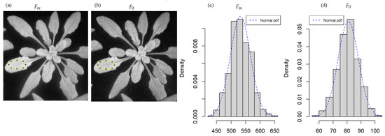
Figure 1. Example of chlorophyll fluorescence images of Arabidopsis thaliana inoculated by a bacteria, at day 2, pot 19, a healthy pot (inoculated with water): (a) $F_m$ maximum fluorescence and (b) $F_0$ minimum fluorescence. The histograms (c,d) are the associated frequency distribution of pixel counts inside the region of interest drawn in a solid yellow line in (a,b), respectively. The dashed blue line in the histograms is the fit with a normal probability density function (pdf).

Therefore, we verified the adequacy of $F_0$ and $F_m$ to a normal distribution with the D’Agostino test [28]. We chose the D’Agostino test among other normality tests since it is the recommended test in case of the presence of ex-aequo in the variable. It’s our case with the number of pixels data. We sample four pots from Healthy and Diseased for each day of the experiment, and we select areas located in the limb of the leaves as illustrated in Figure 1. Table 1 shows the mean and the standard deviation of these four p-values associated with the D’Agostino test of normality on the resulting pixel counts of the selections. From Table 1, all p-values are higher than 0.05. Consequently, we do not reject the null hypothesis that $F_0$ and $F_m$ follow a normal distribution in either healthy or diseased tissues. We extracted the mean and the standard deviation of healthy and diseased pixels from $F_0$ and $F_m$ parameters for the six days of the experiment. The results are in Table 2. It is noticeable that the standard deviation of the Gaussian distribution is relatively stable for healthy and diseased plants over the experiment. This observation is compatible with the interpretation of randomness due mainly to the stationary thermal noise of the camera.

Table 1. Mean ± the standard deviation of four p-values associated with the D’Agostino test of normality in the limb of the Arabidopsis thaliana inoculated by a bacteria for $F_m$ maximum fluorescence and $F_0$ minimum fluorescence. D0, …, and D8 are the six days of the acquisition of chlorophyll fluorescence images.

Time	${\mathit{F}}_{\mathit{m}}$		${\mathit{F}}_0$
	Healthy	Diseased	Healthy	Diseased
D0	0.53 ± 0.33	0.55 ± 0.25	0.59 ± 0.34	0.60 ± 0.33
D2	0.39 ± 0.25	0.59 ± 0.35	0.31 ± 0.25	0.57 ± 0.38
D5	0.60 ± 0.38	0.45 ± 0.31	0.33 ± 0.19	0.31± 0.18
D6	0.30 ± 0.22	0.46 ± 0.23	0.47± 0.33	0.44 ± 0.26
D7	0.27 ± 0.10	0.24 ± 0.19	0.43 ± 0.31	0.44 ± 0.10
D8	0.26 ± 0.16	0.25 ± 0.10	0.25 ± 0.14	0.11 ± 0.04

Table 2. Mean $\mu$, and standard deviation, $\sigma$, values on Healthy and Diseased tissues of chlorophyll fluorescence parameters $F_0$ (minimum fluorescence) and $F_m$ (maximum fluorescence) for images of plants inoculated with bacteria. D0, …, and D8 are the six days of the acquisition of chlorophyll fluorescence images.

Time	${\mathit{\mu }}_{{\mathit{F}}_0}$		${\mathit{\sigma }}_{{\mathit{F}}_0}$		${\mathit{\mu }}_{{\mathit{F}}_{\mathit{m}}}$		${\mathit{\sigma }}_{{\mathit{F}}_{\mathit{m}}}$
	Healthy	Diseased	Healthy	Diseased	Healthy	Diseased	Healthy	Diseased
D0	62.845	42.158	15.261	6.870	418.173	182.367	89.129	33.985
D2	64.756	78.609	16.343	15.380	432.239	338.601	95.681	63.571
D5	67.168	76.984	16.796	21.338	438.586	301.224	96.591	87.018
D6	67.402	77.424	17.150	21.545	444.460	306.174	99.267	86.616
D7	68.781	77.363	17.407	21.546	447.470	306.662	100.153	87.427
D8	67.256	74.562	16.961	21.719	441.044	305.809	98.580	86.968

2.2. Arabidopsis thaliana Infected with a Fungal Pathogen

We considered a second study aiming to score the development of fungal pathogen symptoms (Botrytis cinerea) on the Arabidopsis thaliana plant [12]. This is currently the only public data set on chlorophyll fluorescence imaging with diseased plants that we found. The data set can be found in [29]. It is composed of chlorophyll fluorescences images and RGB images acquired during 96 h post-infection at 0 h, 24 h, 72 h, and 98 h. After checking successfully (not shown) the Gaussianity of the distribution of gray levels in limbs of $F_0$ and $F_m$ images, we computed like for the previous data set the mean and standard deviation associated. The value obtained is provided in Table 3. Here again, one can notice that the standard deviation of the Gaussian distribution is relatively stable over the experiment but only for the healthy plants. For this fungal disease, spores progressively appear at the surface of the leaves. These spores act as a multiplicative filter that absorbs the incident light. The emergence of these spores may add another source of randomness here.

Table 3. Mean $\mu$, and standard deviation, $\sigma$, values on Healthy and Diseased tissues of chlorophyll fluorescence parameters $F_0$ (minimum fluorescence) and $F_m$ (maximum fluorescence) for the data set of plants infected with fungal pathogen data. 0 h, …, 96 h are the five times of the acquisition of chlorophyll fluorescence images.

Time	${\mathit{\mu }}_{{\mathit{F}}_0}$		${\mathit{\sigma }}_{{\mathit{F}}_0}$		${\mathit{\mu }}_{{\mathit{F}}_{\mathit{m}}}$		${\mathit{\sigma }}_{{\mathit{F}}_{\mathit{m}}}$
	Healthy	Diseased	Healthy	Diseased	Healthy	Diseased	Healthy	Diseased
0 h	142.747	-	31.056	-	810.626	-	192.474	-
24 h	122.533	123.685	52.404	77.543	676.331	329.290	275.724	277.567
48 h	105.450	82.616	56.436	66.731	537.056	222.493	295.606	203.232
72 h	121.525	73.177	40.216	42.067	618.474	172.596	225.188	150.189
96 h	103.579	43.691	50.808	41.099	526.299	103.953	274.768	133.111

In the following sections, we will refer to the bacteria data set, the chlorophyll fluorescence images associated with the Arabidopsis thaliana inoculated by a bacteria and by fungal pathogen data set, the chlorophyll fluorescence images of the Arabidopsis thaliana infected with a fungal pathogen.

3. Methods

3.1. Statistical Model of Fv/Fm

In the chlorophyll fluorescence imaging technique, the raw images $F_m$ and $F_0$ are not directly used [30,31]. Instead, they are combined to produce some indices, which serve as a biomarker. We focus on the most common of these indices, known as the maximum quantum yield of photosystem II (PSII) [32]:

$$\frac{F_v}{F_m}=\frac{(F_m-F_0)}{F_m}.$$

(1)

This ratio is an indicator of plant stress and is among the most used chlorophyll fluorescence parameter. It serves as a biomarker to assess the normal or abnormal photosynthetic activity of plant tissue with a threshold applied to the distributions. The choice of this parameter $F_v/F_m$ is made without loss of generality as all of the indices in chlorophyll fluorescence are based on ratios of images with variations concerning the timing of the flash of light and the wavelength.

We have shown that both $F_m$ and $F_0$ can be modeled as Gaussian distribution in the previous section.

Since the Gaussian distribution is alpha-stable, the difference between the two Gaussian distributions is known to be a Gaussian distribution. Consequently, the distribution of $F_v/F_m$ can be modeled in the following way. Let us consider the variables X and Y as $F_0$ and $F_m$, respectively, where X and Y are two identical and independent normal distributions:

$$X\sim N({\mu }_x,{\sigma }_x)\mathrm{and}Y\sim N({\mu }_y,{\sigma }_y).$$

The probability density function, $PZ$, of the ratio $Z=X/Y$ is given by [33,34]:

$$p_Z\left(z\right)=\frac{\rho }{\pi (1+{\rho }^2{z}^2)}exp\left(-\frac{{\rho }^2{\beta }^2+1}{2{\delta }_y^2}\right)\times \left[1+\sqrt{\frac{\pi }{2}}qerf\left(\frac{q}{\sqrt{2}}\right)exp\left(\frac{q^2}{2}\right)\right],$$

(2)

with ${\displaystyle \beta =\frac{{\mu }_x}{{\mu }_y}}$; ${\displaystyle \rho =\frac{{\sigma }_y}{{\sigma }_x}}$; ${\displaystyle {\delta }_y=\frac{{\sigma }_y}{{\mu }_y}}$; ${\displaystyle q=\frac{1+\beta {\rho }^{2}z}{{\delta }_y\sqrt{1+{\rho }^2{z}^2}}}$, and ${\displaystyle erf\left(\frac{q}{\sqrt{2}}\right)=\frac{2}{\sqrt{\pi }}{\int }_0^{\frac{q}{\sqrt{2}}}exp(-t^2)\mathrm{d}t}$.

We can write this $PZ$ otherwise using the confluent hypergeometric function,${}_1{F}_1(.)$ [35]:

$$p_Z\left(z\right)=\frac{\rho }{\pi (1+{\rho }^2{z}^2)}exp\left(-\frac{{\beta }^2{\rho }^2+1}{2{\delta }_y^2}\right){}_1{F}_1\left(1,\frac{1}{2};\frac{1}{2{\delta }_y^2}\frac{{(1+\beta {\rho }^{2}z)}^2}{1+{\rho }^2{z}^2}\right),$$

(3)

with ${}_1{F}_1(.)$, the confluent hypergeometric function, also known as Kummer’s function and defined as follow:

$$\begin{array}{c}\hfill {}_1{F}_1(a;c;z)=\sum _{n=0}^{+\infty }\frac{{\left(a\right)}_n}{{\left(c\right)}_n}\frac{z^n}{n!},\end{array}$$

(4)

where the Pochhammer symbol ${\left(a\right)}_n$ indicates the nth rising factorial of a, i.e.,

$$\begin{array}{c}\hfill {\left(a\right)}_n=a(a+1)\dots (a+n-1)=\frac{{\Gamma }(a+n)}{{\Gamma }\left(a\right)}\mathrm{if}n=1,2,\dots \end{array}$$

If $n=0$, ${\left(a\right)}_n=1$. The demonstration of the second form of the $PZ$ given by Equation (3) is presented in Appendix A.1.

An approximation of the distribution of Z by a normal distribution has been proposed by [34]. Most authors defined conditions on the parameters, $\beta$, $\rho$ and ${\delta }_y$ resulting from empirical or simulation works and showed the switch from a normal distribution to a bimodal distribution under certain values [36,37,38]. This is illustrated with simulation for different values of $\beta$, $\rho$ and ${\delta }_y$ in Figure 2. We draw the distribution of the ratio for three different values of the parameters and we add the normal approximation proposed by [34].

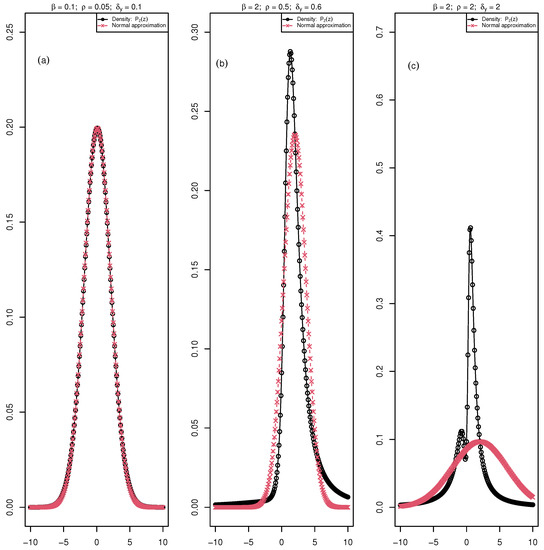
Figure 2. The black curve with circle points is the distribution $PZ$ of the ratio $F_v/F_m$ ($F_m$ maximum fluorescence and $F_v=F_m-F_0$, $F_0$ minimum fluorescence) for an increasing values of the parameters, $\beta$, $\rho$, and ${\delta }_y$ and the red curve with crossed points is the normal approximation of the distribution in each of these cases. (a) A case with perfect fit of the ratio density and the normal approximation; (b) a deviation from normal distribution; (c) a case where the ratio density is bimodal and the normal approximation is not appropriate.

In the first case ($\beta =0.1$, $\rho =0.05$, ${\delta }_y=0.1$), we see a perfect fit of the normal approximation. In the second case ($\beta =2$, $\rho =0.5$, ${\delta }_y=0.6$), we start to see the deviation from normality, whereas for ($\beta =2$, $\rho =2$, ${\delta }_y=2$), the distribution of the ratio is bimodal. Therefore, supposing a normal distribution of $Fv/Fm$ will be more or less wrong depending on the values of $\beta$, $\rho$, and ${\delta }_y$.

There is not a sufficient amount of public sets of chlorophyll fluorescence images to determine if the normal assumption can always be done in estimation of statistical parameters. Therefore, it is necessary to design estimators adapted for the non-Gaussianity of Z in general.

3.2. Estimation of the PZ Parameters

We now present two estimators of the non-Gaussian distribution Z modeling the Maximum Quantum Yield $F_v/F_m$. The first estimator is based on the Bayesian estimation and the second one follows the expectation maximization (EM) algorithm. The Bayesian estimation is chosen here with the hypothesis that two parameters are known according to some prior information and we need to estimate only one parameter. For the EM algorithm, all the parameters are unknown and need to be estimated. We consider that the latter is a more general approach than the former.

3.2.1. Bayesian Estimation

We suppose that $\beta$ and $\rho$ are known, and we aim to estimate ${\delta }_y$ using Bayesian inference. We consider the results for the first day of the experiment as our observed data to get $\beta$ and $\rho$ values. The next step is to define the prior probability for ${\delta }_y$. We recall that ${\delta }_y={\sigma }_y/{\mu }_y$. Since only the parameters of the first day are known (${\mu }_x;{\mu }_y;{\sigma }_x;{\sigma }_y$), we simulate N samples of Y associated to the first day: $Y_1,\dots ,Y_N\sim N({\mu }_y,{\sigma }_y)$. The ratio of the standard deviation to the mean value of these N samples leads to one ${\delta }_y$ value. We repeat this simulation a couple of times (let us say S times) and we define ${\delta }_y\sim N({\mu }_{{\delta }_y},{\sigma }_{{\delta }_y}$), with ${\mu }_{{\delta }_y}$ and ${\sigma }_{{\delta }_y}$ the mean and standard deviation of the ${\delta }_y$ values obtained with the S simulations. The posterior distribution is therefore given by:

$$\begin{array}{cc}\hfill p\left({\delta }_y\right|z_1,\dots ,z_N)& =\frac{p\left({\delta }_y\right)p(z_1,\dots ,z_N|{\delta }_y)}{\underset{-\infty }{\overset{+\infty }{\int }}p\left({\delta }_y\right)p(z_1,\dots ,z_N|{\delta }_y)\mathrm{d}{\delta }_y},\hfill \end{array}$$

where

$$\begin{array}{c}\hfill p(z_1,\dots ,z_N|{\delta }_y)=exp\left(\frac{-N({\rho }^2{\beta }^2+1)}{2{\delta }_y^2}\right)\prod _{i=1}^N\frac{\rho }{\pi (1+{\rho }^2{z}_i^2)}{}_1{F}_1\left(1,\frac{1}{2};\frac{1}{2{\delta }_y^2}\frac{{(1+\beta {\rho }^2{z}_i)}^2}{1+{\rho }^2{z}_i^2}\right),\end{array}$$

(5)

and

$$\begin{array}{cc}\hfill & \underset{-\infty }{\overset{+\infty }{\int }}p\left({\delta }_y\right)p(z_1,\dots ,z_N|{\delta }_y)\mathrm{d}{\delta }_y=\left(\prod _{i=1}^N\frac{\rho }{\pi (1+{\rho }^2{z}_i^2)}\right)\times \hfill \\ \hfill & \underset{-\infty }{\overset{+\infty }{\int }}exp\left(\frac{-N({\rho }^2{\beta }^2+1)}{2{\delta }_y^2}-\frac{{({\delta }_y-{\mu }_{{\delta }_y})}^2}{2{\sigma }_{{\delta }_y}^2}\right)\prod _{i=1}^N{}_1{F}_1\left(1,\frac{1}{2};\frac{1}{2{\delta }_y^2}\frac{{(1+\beta {\rho }^2{z}_i)}^2}{1+{\rho }^2{z}_i^2}\right)\mathrm{d}{\delta }_y,\hfill \end{array}$$

(6)

with $z_1=\frac{X_1}{Y_1},\dots ,z_N=\frac{X_N}{Y_N}$, N ratios of N samples of two normal distributions $X\sim N({\mu }_x,{\sigma }_x)$, and $Y\sim N({\mu }_y,{\sigma }_y)$. Last step is to determine the posterior mean estimator of ${\delta }_y$, which is given by [39]:

$$\begin{array}{cc}\hfill \widehat{{\delta }_y}& =E\left({\delta }_y\right|z_1,\dots ,z_N)\hfill \\ \hfill & =\underset{-\infty }{\overset{+\infty }{\int }}{\delta }_{y}p\left({\delta }_y\right|z_1,\dots ,z_N)\mathrm{d}{\delta }_y.\hfill \end{array}$$

(7)

It is not obvious to compute the above integral since it contains the confluent hypergeometric function. In this case, we use the Monte Carlo (MC) method to numerically approximate this integral. The approximation of ${\delta }_y$ using Monte-Carlo is detailed in Algorithm 1. The resulting quantity is an estimator without bias and highly consistent with ${\delta }_y$. The only drawback of using the MC method is that it is time-consuming. More iterations lead to better consistency but to more simulation time.

3.2.2. EM Estimation of the Parameters

Knowing that the pdf of Z is the result of the ratio of two independent normal distributions N(${\mu }_x,{\sigma }_x$) and N(${\mu }_y,{\sigma }_y$), respectively, we estimate first the parameters $({\mu }_x,{\sigma }_x,{\mu }_y,{\sigma }_y)$ by performing the expectation maximization (EM) algorithm. Thereafter, the parameters $(\beta ,\rho ,{\delta }_y)$ can be deduced from the following relations:

$$\begin{array}{c}\hfill \widehat{\beta }=\frac{{\widehat{\mu }}_x}{{\widehat{\mu }}_y},\widehat{\rho }=\frac{{\widehat{\sigma }}_y}{{\widehat{\sigma }}_x},{\widehat{\delta }}_y=\frac{{\widehat{\sigma }}_y}{{\widehat{\mu }}_y}\end{array}$$

(8)

Consider N independent and identically distributed realizations $z_i,i=\{1,\dots ,N\}$ of a random variable Z distributed according to the $PZ$ written with the confluent hypergeometric function (3). This form of the $PZ$ is more adequate to the estimation parameter procedure using the EM algorithm.

The pdf associated to the ratio Z depends on the set of unknown parameters: $\theta =({\mu }_x,{\mu }_y,{\sigma }_x^2,{\sigma }_y^2)$. The maximum likelihood estimator $\widehat{\theta }$ of the set parameter $\theta$, is given by:

$$\begin{array}{cc}\hfill {\widehat{\theta }}_{ML}& =arg\underset{\theta }{max}{p}_Z\left(z\right|\theta )=arg\underset{\theta }{max}\prod _{i=1}^N{p}_Z\left(z_i\right|\theta ).\hfill \end{array}$$

(9)

Algorithm 1: MC estimation of ${\delta }_y$.

Input: $N,S,K$ Output: $\widehat{{\delta }_y}$   Loop: K iteration:   Repeat for k in $1\dots K$     Loop: S iteration:     Initialization:     Set the parameters $({\mu }_x,{\sigma }_x,{\mu }_y,{\sigma }_y)$ of the first day of the experiment     Repeat     generate N samples $y_1,\dots ,y_N\sim N({\mu }_y,{\sigma }_y)$     calculate the associated mean ${\mu }_y^s$ and standard deviation ${\sigma }_y^s$:        ${\mu }_y^s=\frac{1}{N}{\sum }_{i=1}^N{y}_i$ and ${\sigma }_y^s=\sqrt{\frac{1}{N}{\sum }_{i=1}^N{(y_i-{\mu }_y^s)}^2}$, for $s=1,\dots ,S$     deduce ${\delta }_y^s=\frac{{\sigma }_y^s}{{\mu }_y^s}$, for $s=1,\dots ,S$     generate N samples $x_1,\dots ,x_N\sim N({\mu }_x,{\sigma }_x)$     compute N samples $z_1=\frac{x_1}{y_1},\dots ,z_N=\frac{x_N}{y_N}$     deduce $p(z_1,\dots ,z_N|{\delta }_y^s)$, for $s=1,\dots ,S$ using Equation (5)     End loop     calculate ${\mu }_{{\delta }_y}=\frac{1}{S}{\sum }_{s=1}^S{\delta }_y^s$ and ${\sigma }_{{\delta }_y}=\sqrt{\frac{1}{S}{\sum }_{s=1}^S{({\delta }_y^s-{\mu }_{{\delta }_y})}^2}$     deduce $p\left({\delta }_y^s\right)$ the pdf of ${\delta }_y^s\sim N({\mu }_{{\delta }_y},{\sigma }_{{\delta }_y})$, for $s=1,\dots ,S$     Return ${\displaystyle \widehat{{\delta }_y^k}=\frac{{\sum }_{s=1}^S{\delta }_y^s\times p\left({\delta }_y^s\right)\times p(z_1,\dots ,z_N|{\delta }_y^s)}{{\sum }_{s=1}^{S}p\left({\delta }_y^s\right)\times p(z_1,\dots ,z_N|{\delta }_y^s)}}$.   Save $\widehat{{\delta }_y^k}$ the result of the last return for k from 1 to K.   Return ${\displaystyle \widehat{{\delta }_y}=\frac{1}{K}\sum _{k=1}^K\widehat{{\delta }_y^k}}$;

In the absence of an explicit solution of the maximum likelihood Equation (9), the Expectation–Maximization (EM) algorithm is used to find an estimation $\widehat{\theta }$ given a current estimate ${\theta }^{\prime }$ of $\theta$. We suppose that for each observed $z_i$ an unobserved and hidden data $y_i$ is associated. The sequence $\{y_i,i=1,\dots ,N\}$ is also supposed to be independent and identically distributed.

$$\begin{array}{ccc}\hfill \widehat{\theta }& =& arg\underset{\theta }{max}{E}_{Y|Z}\{ln{f}_{Y,Z}(Z,Y|\theta )|z,{\theta }^{\prime }\}\hfill \\ & =& arg\underset{\theta }{max}{E}_{Y|Z}\{ln\prod _{i=1}^N{f}_{Y,Z}(Z_i,Y_i|\theta )|z_i,{\theta }^{\prime }\}\hfill \\ & =& arg\underset{\theta }{max}{E}_{Y|Z}\{\sum _{i=1}^{N}ln{f}_{Y,Z}(Z_i,Y_i|\theta )|z_i,{\theta }^{\prime }\}\hfill \\ & =& arg\underset{\theta }{max}\sum _{i=1}^N{E}_{Y|Z}\{ln{f}_{Y,Z}(Z_i,Y_i|\theta )|z_i,{\theta }^{\prime }\}.\hfill \end{array}$$

(10)

Let ${\theta }_x=({\mu }_x,{\sigma }_x)$ and ${\theta }_y=({\mu }_y,{\sigma }_y)$. By using the fact that:

$$f_{Y,Z}(z_i,y_i|\theta )=f_{Z|Y}\left(z_i\right|y_i,{\theta }_x)f_Y\left(y_i\right|{\theta }_y),$$

(11)

then (10) can be maximized separately in respect to the set of parameters ${\theta }_x$ and ${\theta }_y$ as follows:

$$\begin{array}{cc}\hfill & {\widehat{\theta }}_x=arg\underset{{\theta }_x}{max}\sum _{i=1}^N{E}_{Y|Z}\{ln{f}_{Z|Y}\left(Z_i\right|Y_i,{\theta }_x)|z_i,{\theta }^{\prime }\}\hfill \end{array}$$

(12)

$$\begin{array}{cc}\hfill & {\widehat{\theta }}_y=arg\underset{{\theta }_y}{max}\sum _{i=1}^N{E}_{Y|Z}\{ln{f}_Y\left(Y_i\right|{\theta }_y)|z_i,{\theta }^{\prime }\}.\hfill \end{array}$$

(13)

By developing these two equations, and differentiating with respect to ${\mu }_x$, ${\sigma }_x$, ${\mu }_y$ and ${\sigma }_y$ (Appendix A.2), we provide the estimate ${\widehat{\theta }}_x=({\mu }_x,{\sigma }_x)$ and ${\widehat{\theta }}_y=({\mu }_y,{\sigma }_y)$:

$$\begin{array}{cc}\hfill {\widehat{\mu }}_x& =\frac{1}{N}\sum _{i=1}^N{z}_i{E}_{Y|Z}\left\{Y_i\right|z_i,{\theta }^{\prime }\}\hfill \end{array}$$

(14)

$$\begin{array}{cc}\hfill {\widehat{\sigma }}_x^2& =\frac{1}{N}\sum _{i=1}^N{z}_i^2{E}_{Y|Z}\left\{Y_i^2\right|z_i,{\theta }^{\prime }\}-{\widehat{\mu }}_x^2\hfill \end{array}$$

(15)

$$\begin{array}{cc}\hfill {\widehat{\mu }}_y& =\frac{1}{N}\sum _{i=1}^N{E}_{Y|Z}\left\{Y_i\right|z_i,{\theta }^{\prime }\}\hfill \end{array}$$

(16)

$$\begin{array}{cc}\hfill {\widehat{\sigma }}_y^2& =\frac{1}{N}\sum _{i=1}^N{E}_{Y|Z}\left\{Y_i^2\right|z_i,{\theta }^{\prime }\}-{\widehat{\mu }}_y^2.\hfill \end{array}$$

(17)

where $E_{Y|Z}\left\{Y_i\right|z_i,{\theta }^{\prime }\}$ and $E_{Y|Z}\left\{Y_i^2\right|z_i,{\theta }^{\prime }\}$ are the posterior expectation values dependent of the distribution of Y given by:

$$\begin{array}{cc}\hfill E_{Y|Z}\left\{Y_i\right|z_i,{\theta }^{\prime }\}& =\frac{\gamma }{\mu }\frac{{}_1{F}_1\left(2,\frac{3}{2};\frac{{\gamma }^2}{4\mu }\right)}{{}_1{F}_1\left(1,\frac{1}{2};\frac{{\gamma }^2}{4\mu }\right)},\hfill \end{array}$$

(18)

and

$$\begin{array}{cc}\hfill E_{Y|Z}\left\{Y_i^2\right|z_i,{\theta }^{\prime }\}& =\frac{1}{\mu }\frac{{}_1{F}_1\left(2,\frac{1}{2};\frac{{\gamma }^2}{4\mu }\right)}{{}_1{F}_1\left(1,\frac{1}{2};\frac{{\gamma }^2}{4\mu }\right)},\hfill \end{array}$$

(19)

with ${\displaystyle \mu =\frac{1}{2}\left(\frac{z_i^2}{{\sigma }_x^2}+\frac{1}{{\sigma }_y^2}\right)}$ and ${\displaystyle \gamma =\frac{{\mu }_y}{{\sigma }_y^2}+\frac{{\mu }_x}{{\sigma }_x^2}{z}_i}$.

The proof of both these expressions is also in Appendix A.2. This leads to the following iterative Algorithm 2 for solving the maximum likelihood problem:

3.3. Comparison with Normal Assumptions Baseline

To show the benefit of using the Bayesian and EM estimations with the $PZ$ distribution, we compare them with a standard normal distribution assumption and the normal approximation proposed in [34].

3.4. Numerical Experiments

We now present the metrics used to establish the value of the proposed non-Gaussian estimator for $PZ$. We then describe the numerical simulation undertaken with these metrics.

Algorithm 2: EM algorithm.

Input: $N,z_i,ϵ$ Output: $\widehat{\theta }=({\widehat{\mu }}_x,{\widehat{\sigma }}_x,{\widehat{\mu }}_y,{\widehat{\sigma }}_y)$ and consequently ($\widehat{\beta },\widehat{\rho },{\widehat{\delta }}_y)$    Initialization:    Set the parameters ${\theta }^{\prime }=({\mu }_x^{\prime },{\sigma }_x^{\prime },{\mu }_y^{\prime },{\sigma }_y^{\prime })$    Loop:    Repeat    Calculate ${\mu }^{\prime }=\frac{1}{2}\left(\frac{z_i^2}{{\sigma }_x^{\prime 2}}+\frac{1}{{\sigma }_y^{\prime 2}}\right)$ and ${\gamma }^{\prime }=\frac{{\mu }_y^{\prime }}{{\sigma }_y^{\prime 2}}+\frac{{\mu }_x^{\prime }}{{\sigma }_x^{\prime 2}}{z}_i$    Estimate ${\widehat{\mu }}_x=\frac{1}{N}{\sum }_{i=1}^N{z}_i\frac{{\gamma }^{\prime }}{{\mu }^{\prime }}\frac{{}_1{F}_1\left(2,\frac{3}{2};\frac{{\gamma }^{\prime 2}}{4{\mu }^{\prime }}\right)}{{}_1{F}_1\left(1,\frac{1}{2};\frac{{\gamma }^{\prime 2}}{4{\mu }^{\prime }}\right)}$    Estimate ${\widehat{\sigma }}_x^2=\frac{1}{N}{\sum }_{i=1}^N{z}_i^2\frac{1}{{\mu }^{\prime }}\frac{{}_1{F}_1\left(2,\frac{1}{2};\frac{{\gamma }^{\prime 2}}{4{\mu }^{\prime }}\right)}{{}_1{F}_1\left(1,\frac{1}{2};\frac{{\gamma }^{\prime 2}}{4{\mu }^{\prime }}\right)}-{\widehat{\mu }}_x^2$    Estimate ${\widehat{\mu }}_y=\frac{1}{N}{\sum }_{i=1}^N\frac{{\gamma }^{\prime }}{{\mu }^{\prime }}\frac{{}_1{F}_1\left(2,\frac{3}{2};\frac{{\gamma }^{\prime 2}}{4{\mu }^{\prime }}\right)}{{}_1{F}_1\left(1,\frac{1}{2};\frac{{\gamma }^{\prime 2}}{4{\mu }^{\prime }}\right)}$    Estimate ${\widehat{\sigma }}_y^2=\frac{1}{N}{\sum }_{i=1}^N\frac{1}{{\mu }^{\prime }}\frac{{}_1{F}_1(2,\frac{1}{2};\frac{{\gamma }^{\prime 2}}{4{\mu }^{\prime }})}{{}_1{F}_1(1,\frac{1}{2};\frac{{\gamma }^{\prime 2}}{4{\mu }^{\prime }})}-{\widehat{\mu }}_y^2$    Calculate the stop criterion: $D\leftarrow \parallel \widehat{\theta }-{\theta }^{\prime }\parallel$    Define the next iteration initialization: ${\mu }_x^{\prime },{\sigma }_x^{\prime },{\mu }_y^{\prime },{\sigma }_y^{\prime }\leftarrow {\widehat{\mu }}_x,{\widehat{\sigma }}_x,{\widehat{\mu }}_y,{\widehat{\sigma }}_y$    Until $D<ϵ$    Return ${\displaystyle \widehat{\beta }=\frac{{\widehat{\mu }}_x}{{\widehat{\mu }}_y}}$; ${\displaystyle \widehat{\rho }=\frac{{\widehat{\sigma }}_y}{{\widehat{\sigma }}_x}}$; ${\displaystyle {\widehat{\delta }}_y=\frac{{\widehat{\sigma }}_y}{{\widehat{\mu }}_y}}$;

3.4.1. Fractional Moments

Dividing two normal distributions lead to a high variability of the mean value. This problem has been raised in agricultural research [40]. For a coefficient of variation of Y ($C{V}_Y$) strictly lower than 0.2, the mean value of the ratio is stable. The coefficient of variation of Y is equal to ${\delta }_y$: the ratio of the standard deviation to the mean of Y. Thus, we used interchangeably ${\delta }_y$ or $C{V}_Y$. For the bacteria data set, ${\delta }_y$ values are between 0.2 and 0.3 (see Table 4), and for the fungal pathogen data set, ${\delta }_y$ values are between 0.8 and 1.3 (see Table 5). Therefore, we are not in a situation with a stable mean ratio. We propose an alternative for the mean value in these cases. We suggest using the mean of the fractional moment.

Table 4. The values of $\beta$, $\rho$ and ${\delta }_y$ associated with the fluorescence data on Healthy and Diseased plants of the bacteria data set. D0, …, and D8 are the six days of the acquisition of chlorophyll fluorescence images.

Time	$\mathit{\beta }$		$\mathit{\rho }$		${\mathit{\delta }}_{\mathit{y}}$
	Healthy	Diseased	Healthy	Diseased	Healthy	Diseased
D0	0.150	0.231	5.840	4.947	0.213	0.186
D2	0.150	0.232	5.855	4.133	0.221	0.188
D5	0.153	0.256	5.751	4.078	0.220	0.289
D6	0.152	0.253	5.788	4.020	0.223	0.283
D7	0.154	0.252	5.753	4.058	0.224	0.285
D8	0.152	0.244	5.812	4.004	0.224	0.284

Table 5. The values of $\beta$, $\rho$ and ${\delta }_y$ associated with the fluorescence data on Healthy and Diseased plants of the fungal pathogen data set. 0 h, …, 96 h are the five times of the acquisition of chlorophyll fluorescence images.

Time	$\mathit{\beta }$		$\mathit{\rho }$		${\mathit{\delta }}_{\mathit{y}}$
	Healthy	Diseased	Healthy	Diseased	Healthy	Diseased
0 h	0.176		6.198		0.237
24 h	0.181	0.376	5.262	3.580	0.408	0.843
48 h	0.196	0.371	5.238	3.046	0.550	0.913
72 h	0.196	0.424	5.599	3.570	0.364	0.870
96 h	0.197	0.420	5.408	3.239	0.522	1.280

We give the expression for these moments that benefits from the independence of the variability of the denominator. The fractional moments expression is given by:

$$\begin{array}{cc}\hfill E\left\{\right|Z{|}^s\}& ={\left(\frac{{\sigma }_x}{{\sigma }_y}\right)}^s\frac{\mathsf{\Gamma }(1-s)\mathsf{\Gamma }(1+s)}{\mathsf{\Gamma }(1-\frac{s}{2})\mathsf{\Gamma }(1+\frac{s}{2})}{}_1{F}_1\left(\frac{s}{2},\frac{1}{2},-\frac{{\mu }_y^2}{2{\sigma }_y^2}\right){}_1{F}_1\left(\frac{-s}{2},\frac{1}{2},-\frac{{\mu }_x^2}{2{\sigma }_x^2}\right)\hfill \end{array}$$

(20)

$$\begin{array}{cc}\hfill & ={\rho }^{-s}\frac{\mathsf{\Gamma }(1-s)\mathsf{\Gamma }(1+s)}{\mathsf{\Gamma }(1-\frac{s}{2})\mathsf{\Gamma }(1+\frac{s}{2})}{}_1{F}_1\left(\frac{s}{2},\frac{1}{2},-\frac{1}{2{\delta }_y^2}\right){}_1{F}_1\left(\frac{-s}{2},\frac{1}{2},-\frac{1}{2{\delta }_x^2}\right)\hfill \end{array}$$

(21)

with $\beta =\frac{{\mu }_x}{{\mu }_y},\rho =\frac{{\sigma }_y}{{\sigma }_x},{\delta }_x=\frac{{\sigma }_x}{{\mu }_x},{\delta }_y=\frac{{\sigma }_y}{{\mu }_y}$. The proof of this expression is given in Appendix A.4 for $0<s<1$.

3.4.2. Monte Carlo Experiments

To have ground truth in the evaluation of the value of the estimator of $PZ$, we resorted to the use of simulation of the two empirical data sets both in the healthy and diseased plants. We considered the size of the smallest leaves and the largest ones on our two data sets. We found 10 pixels for the smallest leaves and 80 for the largest ones. Generation of Gaussian distribution for $F_m$ and $F_0$ mimicking the experimental observation of our two experimental data sets given in Table 2 and Table 3. The resulting observations of $F_v/F_m$ were computed. The two proposed non-Gaussian estimators and the Gaussian baselines estimator described in the previous section were computed. Simulations were repeated 5000 times to compute average performance and associated standard deviations. The end point of our experiments is the relative error:

$$RE=\frac{Measured-Estimated}{Estimated}$$

.

The measured value is the exact value of the fractional moment, and the estimated value is obtained with one of the compared estimators. This comparison is made at all dates of the experimental data used for the simulation. The prior values used in our proposed methods are initialized with the values of the first day of the experiment.

4. Results

We are now ready to assess the importance of non-Gaussianity in chlorophyll fluorescence images via the comparison of the relative error of our two proposed statistical estimators against the standard estimator under Gaussian assumptions.

4.1. Arabidopsis thaliana Inoculated by a Bacteria

To illustrate the non-Gaussianity of the bacteria data set, we provide the distribution of $PZ$ for the mean values of $\beta$, $\rho$, and ${\delta }_y$ over the six days of our real experimental data set both for Healthy and Diseased in Figure 3. The normal approximation is added. One can observe a small deviation from Gaussianity.

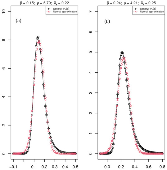
Figure 3. The distribution $PZ$ of the ratio $F_v/F_m$ ($F_m$ maximum fluorescence and $F_v=F_m-F_0$, $F_0$ minimum fluorescence) is the black curve with circle points, and the normal approximation is the red curve with crossed points. The parameters $\beta$, $\rho$, and ${\delta }_y$ of the distribution $PZ$ are associated with the mean value of these parameters over the six days of the acquisition of chlorophyll fluorescence images for (a) Healthy: $\beta =0.15$, $\rho =5.79$ and ${\delta }_y=0.22$ and (b) Diseased: $\beta =0.24$, $\rho =4.21$ and ${\delta }_y=0.25$ plants of the bacteria data set.

We considered the second-order fractional moment of $PZ$ for this first data set since it led to stable results of the mean of fractional moments for the values of ${\delta }_y$ between 0.3 and 1 (see Appendix A.5). We calculated these second-order fractional moments of $PZ$ for each day of the experiment (Table 6). These are the measured values to which we will compare the estimated values obtained with the Monte Carlo simulations with 10 and 80 samples. The results of the Monte Carlo simulation are given in Table 7. The normal distribution and the normal approximation are the methods of estimation when assuming a normal distribution of $F_v/F_m$. Bayesian and EM estimation are the two proposed non-Gaussian estimators with $PZ$ distribution.

Table 6. Second-order fractional moment of $PZ$ distribution of the ratio for the healthy and diseased leaves of the bacteria data set. D0, …., and D8 are the six days of the acquisition of chlorophyll fluorescence images.

Plants	Time
	D0	D2	D5	D6	D7	D8
Healthy	0.608	0.608	0.604	0.606	0.603	0.605
Diseased	0.514	0.514	0.478	0.482	0.483	0.492

Table 7. The mean value ($\mu$) and the associated standard deviation ($\sigma$) of the second-order fractional moment of the Monte Carlo simulation for 10 and 80 sample sizes, with the first day of the experiment as a reference value, with the assumptions of Gaussian probability density function and the Gaussian approximation proposed in [34] and with the two non-Gaussian estimators, Bayesian and EM.

Method of Estimation	Plants, Sample Size (N)
	Healthy,		Healthy,		Diseased,		Diseased,
	$\mathbf{N}=\mathbf{10}$		$\mathbf{N}=\mathbf{80}$		$\mathbf{N}=\mathbf{10}$		$\mathbf{N}=\mathbf{80}$
	$\mathbf{\mu }$	$\mathbf{\sigma }$	$\mathbf{\mu }$	$\mathbf{\sigma }$	$\mathbf{\mu }$	$\mathbf{\sigma }$	$\mathbf{\mu }$	$\mathbf{\sigma }$
Normal distribution	0.591	0.037	0.613	0.009	0.524	0.016	0.523	0.007
Normal approximation	0.618	0.021	0.618	0.007	0.523	0.019	0.523	0.007
Bayesian estimation	0.608	0.022	0.608	0.008	0.515	0.020	0.514	0.007
EM estimation	0.612	0.017	0.608	0.008	0.516	0.021	0.513	0.008

With both measured (Table 6) and estimated values (Table 7), we calculate the relative error for each day of the experiment. The mean value of the relative error over the six days of the experiment is given in Table 8, for Healthy and Diseased plants, and per sample size.

Table 8. Mean value of the relative error ( % ) for the five days of the experiment per method of estimation and per sample size, N, for Healthy and Diseased plants of the bacteria data set.

Method of Estimation	Plants, Sample Size (N)
	Healthy,	Healthy,	Diseased,	Diseased,
	$\mathbf{N}=\mathbf{10}$	$\mathbf{N}=\mathbf{80}$	$\mathbf{N}=\mathbf{10}$	$\mathbf{N}=\mathbf{80}$
Normal distribution	2	1	6	6
Normal approximation	2	2	6	6
Bayesian estimation	0	0	4	4
EM estimation	1	0	5	4

The maximum value of the relative error was not high: 6% with normal assumptions. The relative error is lower for Healthy compared to Diseased plants. Overall, we have a lower error with Bayesian and EM estimations compared to the normal distribution and normal approximation.

4.2. Arabidopsis thaliana Infected with a Fungal Pathogen

We apply the same analysis to the fluorescence images of Arabidopsis thaliana infected with a fungal pathogen. We start with a representation of the distribution of $PZ$ associated with the mean values of $\beta$, $\rho$, and ${\delta }_y$ over the five dates of the empirical data set for both Healthy and Diseased plants, Figure 4.

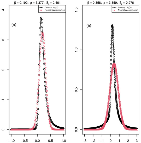
Figure 4. The distribution $PZ$ of the ratio $F_v/F_m$ ($F_m$ maximum fluorescence and $F_v=F_m-F_0$, $F_0$ minimum fluorescence) is the black curve with circle points, and the normal approximation is the red curve with crossed points. The parameters $\beta$, $\rho$, and ${\delta }_y$ of the distribution $PZ$ are associated with the mean value of these parameters over the six days of the acquisition of chlorophyll fluorescence images for (a) Healthy: $\beta =0.192$, $\rho =5.377$ and ${\delta }_y=0.461$ and (b) Diseased: $\beta =0.358$, $\rho =3.359$ and ${\delta }_y=0.976$ plants of the fungal pathogen data set.

The deviation from normality is more pronounced with this data set. We calculate the measured values of the fourth-order fractional moment of $F_v/F_m$ for each date of the experiment (Table 9). The choice to use the fourth order is due to the higher values of ${\delta }_y$ in this data set. Thus, a lower value of the fractional moment was more appropriate (cf. simulation of $C{V}_y$ in Appendix A.5). We then calculate the mean value of the fourth-order fractional moment with the Monte-Carlo simulations for 10 and 80 sample sizes. The simulation results are in Table 10. The mean values represent the estimated fourth-order fractional moment with the four methods of estimation: normal distribution assumption, the normal approximation, and the two non-Gaussian estimators, Bayesian and EM.

Table 9. Fourth-order fractional moment of $PZ$ distribution of the ratio for the Healthy and Diseased plants of the fungal pathogen data set. 0 h, …, 96 h are the five times of the acquisition of chlorophyll fluorescence images.

Plants	Time
	0 h	24 h	48 h	72 h	96 h
Healthy	0.349	0.335	0.304	0.322	0.306
Diseased	-	0.165	0.168	0.138	0.157

Table 10. The mean value ($\mu$) and the associated standard deviation ($\sigma$) of the fourth-order fractional moment of the Monte Carlo simulation with 24 h as a reference value.

Method of Estimation	Plants, Sample Size (N)
	Healthy,		Healthy,		Diseased,		Diseased,
	$\mathbf{N}=\mathbf{10}$		$\mathbf{N}=\mathbf{80}$		$\mathbf{N}=\mathbf{10}$		$\mathbf{N}=\mathbf{80}$
	$\mathbf{\mu }$	$\mathbf{\sigma }$	$\mathbf{\mu }$	$\mathbf{\sigma }$	$\mathbf{\mu }$	$\mathbf{\sigma }$	$\mathbf{\mu }$	$\mathbf{\sigma }$
Normal distribution	0.399	0.037	0.277	0.018	0.284	0.053	0.055	0.025
Normal approximation	0.370	0.035	0.369	0.012	0.231	0.055	0.231	0.019
Bayesian estimation	0.337	0.047	0.334	0.018	0.167	0.107	0.165	0.038
EM estimation	0.327	0.070	0.334	0.017	0.163	0.106	0.165	0.037

We calculate the relative error per time of experiment with the measured value of the fourth-order fractional moment (Table 9) and the estimated values (Table 10). We give in Table 11 the mean value of the relative error over all the experiment acquisition times.

Table 11. Mean value of the relative error (%) for the five times of the experiment per method of estimation and per number of observations for Healthy and Diseased plants of the fungal pathogen data set.

Method of Estimation	Plants, Sample Size (N)
	Healthy,	Healthy,	Diseased,	Diseased,
	$\mathbf{N}=\mathbf{10}$	$\mathbf{N}=\mathbf{80}$	$\mathbf{N}=\mathbf{10}$	$\mathbf{N}=\mathbf{80}$
Normal distribution	26	12	82	65
Normal approximation	17	17	48	48
Bayesian estimation	7	6	7	7
EM estimation	5	6	6	7

We see clearly on the fungal data set that the relative error is much higher if one supposes a normal distribution of the ratio: 26% for healthy ($N=10$) and 82% for diseased ($N=10$) v.s around 6% and 7% for Bayesian and EM estimations. Thus, these results show that using a normal distribution or normal approximation of the ratio $F_v/F_m$ leads to more or less wrong results depending on how pronounced is the deviation from Gaussianity.

5. Discussion

We have quantified the importance of considering the non-Gaussianity in the maximum quantum yield of photosystem II. This non-Gaussianity was only recently highlighted empirically in [12]. In most of the recent studies using the maximum quantum yield of photosystem II as phenotyping characteristic [14,15,17,18,19,20,21,22,24,25,26], the results are presented with average and standard deviation. Our mathematical study shows that this may not be the most appropriate approach especially when the distribution of the gray levels in $F_v/F_m$ strongly deviates from Gaussianity. This advocate for the use of box plots like in [23] to easily visualize the non-Gaussianity. The only use of average and standard deviation in [14,15,17,18,19,20,21,22,24,25,26] was not problematic as the maximum quantum yield of photosystem II is not used as a biomarker for its absolute value but rather to differentiate different phenotypes. However, our mathematical models show that the distribution can be nonsymmetric with heavy tails. This may explain why advanced models have been used in the literature for decision making with decisions trees [41,42] or Gaussian mixtures [12,13] for decision making. We focus on estimation in this article which is distinct from detection. It could be an interesting perspective to compare the advanced approaches [12,13,41,42] with a simple single threshold to be applied to the non-Gaussian distribution considered in our work.

6. Conclusions

In this article, we have demonstrated the importance to consider mathematically the non-Gaussianity of vegetation indices composed of a ratio of images corrupted by Gaussian noises. This was illustrated and detailed with chlorophyll fluorescence images. We have designed estimators adapted to this non-Gaussianity under the hypothesis of independence of the distribution of the images used in the ratio. Despite the simplicity of this model, the benefits of this approach by comparison with the usual Gaussian assumption was demonstrated.

In this work, we focused on estimating the distribution parameters of the ratio $F_v/F_m$ used in chlorophyll fluorescence indices. In the two chlorophyll fluorescence, infected plants data sets that we considered, the distribution of this ratio $F_v/F_m$ didn’t follow a normal distribution. If more chlorophyll fluorescence data sets are available, it could be interesting to have a range of the parameters for the density distribution of the ratio and to identify the intervals for these parameters where normality is verified.

This work could be extended in various directions. Many vegetation indices include a ratio of images and therefore could benefit from the approach proposed in the article. With the two empirical data sets considered, the deviation from Gaussianity was limited, but it was enough to show the importance to use adapted non-Gaussian models. Theoretically, the deviation from Gaussianity can be severe. Therefore, it is fundamentally important to have mathematically grounded estimators. The assumption of independence of the images is a current limitation of our approach that produced lower error but yet biased estimators, especially for small leaves (with a small number of observations). It would be interesting to design models of covariance between images used in the vegetation indices ratio in order to propose possibly unbiased estimators independently of the size of the leaves.

Appendix A.1. Ratio Distribution

The aim of this appendix is to show the passage from the distribution of the ratio written as Equation (2) to the distribution of the ratio written with the hypergeometric function Equation (3). We start by recalling two equalities that will be used hereinafter in the proof.

Prerequisite A1 ([43], Section 3.462, Equation (5)).

$$\begin{array}{cc}\hfill {\int }_0^{\infty }x{e}^{-\mu x^2-2\lambda x}\mathrm{d}x& =\frac{1}{2\mu }\left[1-\lambda \sqrt{\frac{\pi }{\mu }}{e}^{\frac{{\lambda }^2}{\mu }}\left(1-erf\left(\frac{\lambda }{\sqrt{\mu }}\right)\right)\right],\mathit{Real}\left(\mu \right)>0\hfill \end{array}$$

(A1)

Since $erf(.)$ function is an odd function, it follows:

$$\begin{array}{cc}\hfill {\int }_0^{\infty }x{e}^{-\mu x^2-2\lambda x}\mathrm{d}x+{\int }_0^{\infty }x{e}^{-\mu x^2+2\lambda x}\mathrm{d}x& =\frac{1}{\mu }\left[1+\sqrt{\pi \frac{{\lambda }^2}{\mu }}{e}^{\frac{{\lambda }^2}{\mu }}erf\left(\frac{\lambda }{\sqrt{\mu }}\right)\right]\hfill \end{array}$$

(A2)

Prerequisite A2 ([43], Section 3.462, Equation (1)).

$$\begin{array}{cc}\hfill {\int }_0^{\infty }{x}^{\nu -1}{e}^{-\mu x^2-\gamma x}\mathrm{d}x& ={\left(\frac{1}{2\mu }\right)}^{\frac{\nu }{2}}\mathsf{\Gamma }\left(\nu \right)e^{\frac{{\gamma }^2}{8\mu }}{D}_{-\nu }\left(\frac{\gamma }{\sqrt{2\mu }}\right),\mathit{Real}\left(\mu \right)>0,\mathit{real}\left(\nu \right)>0\hfill \end{array}$$

(A3)

with $D_{-\nu }\left(z\right)$ the parabolic cylinder function defined as follow:

$$\begin{array}{cc}\hfill D_{-\nu }\left(z\right)& =2^{-\frac{\nu }{2}}{e}^{-\frac{z^2}{4}}\left[\frac{\sqrt{\pi }}{\mathsf{\Gamma }\left(\frac{1+\nu }{2}\right)}{}_1{F}_1\left(\frac{\nu }{2},\frac{1}{2};\frac{z^2}{2}\right)-\frac{\sqrt{2\pi }}{\mathsf{\Gamma }\left(\frac{\nu }{2}\right)}z{}_1{F}_1\left(\frac{1+\nu }{2},\frac{3}{2};\frac{z^2}{2}\right)\right],\hfill \end{array}$$

$\mathsf{\Gamma }\left(\nu \right)$ is the gamma function and ${}_1{F}_1(.)$ is the confluent hypergeometric function.

Proof. 

Set $X\sim \mathcal{N}({\mu }_x,{\sigma }_x)$ and $Y\sim \mathcal{N}({\mu }_y,{\sigma }_y)$. We will start by proving the probability distribution of the ratio $Z=X/Y$ since, at one step of the proof, the switch to the hypergeometric function will be realised. We denote by $g(z,y)$ the pdf of the joint two random variables $(Z=X/Y,Y=Y)$. It is given as following:

$$\begin{array}{c}\hfill g(z,y)=f(x,y)|\frac{\partial (z,y)}{\partial (x,y)}{|}^{-1},\end{array}$$

(A4)

where the Jacobian determinant of the change of variables is given by $\left|J\right|=\left|\frac{\partial (z,y)}{\partial (x,y)}\right|$ and calculated as follow: $\left|J\right|=\left|\begin{array}{cc}\frac{\partial z}{\partial x}& \frac{\partial z}{\partial y}\\ \frac{\partial y}{\partial x}& \frac{\partial y}{\partial y}\end{array}\right|=\left|\begin{array}{cc}\frac{1}{y}& -\frac{x}{y^2}\\ 0& 1\end{array}\right|=|\frac{1}{y}|$.

Therefore,

$$\begin{array}{c}\hfill g(z,y)=\left|y\right|f(x,y).\end{array}$$

(A5)

The probability distribution of the ratio $Z=X/Y$, denoted $p_Z\left(z\right)$, is given by:

$$\begin{array}{c}\hfill p_Z\left(z\right)={\int }_{-\infty }^{\infty }g(z,y)\mathrm{d}y={\int }_{-\infty }^{\infty }\left|y\right|f(x,y)\mathrm{d}y.\end{array}$$

(A6)

Since the two random variables X and Y are independent then $f(x,y)=f_X\left(x\right)f_Y\left(y\right)$. The expression of $p_Z\left(z\right)$ is then given by

$$\begin{array}{cc}\hfill p_Z\left(z\right)& ={\int }_{-\infty }^{\infty }\left|y\right|f_X\left(x\right)f_Y\left(y\right)\mathrm{d}y\hfill \\ \hfill & ={\int }_{-\infty }^{\infty }\left|y\right|f_X\left(zy\right)f_Y\left(y\right)\mathrm{d}y,\sin \mathrm{ce}x=zy\hfill \\ \hfill & =\frac{1}{2\pi {\sigma }_x{\sigma }_y}{\int }_{-\infty }^{\infty }\left|y\right|e^{-\frac{{(zy-{\mu }_x)}^2}{2{\sigma }_x^2}}{e}^{-\frac{{(y-{\mu }_y)}^2}{2{\sigma }_y^2}}\mathrm{d}y\hfill \\ \hfill & =\frac{1}{2\pi {\sigma }_x{\sigma }_y}{e}^{-\frac{1}{2}\left(\frac{{\mu }_x^2}{{\sigma }_x^2}+\frac{{\mu }_y^2}{{\sigma }_y^2}\right)}{\int }_{-\infty }^{\infty }\left|y\right|e^{-\frac{1}{2}\left(\frac{z^2}{{\sigma }_x^2}+\frac{1}{{\sigma }_y^2}\right)y^2+\left(\frac{{\mu }_x}{{\sigma }_x^2}z+\frac{{\mu }_y}{{\sigma }_y^2}\right)y}\mathrm{d}y\hfill \\ \hfill & =\frac{1}{2\pi {\sigma }_x{\sigma }_y}{e}^{-\frac{1}{2}\left(\frac{{\mu }_x^2}{{\sigma }_x^2}+\frac{{\mu }_y^2}{{\sigma }_y^2}\right)}\left[{\int }_0^{\infty }y{e}^{-\frac{1}{2}\left(\frac{z^2}{{\sigma }_x^2}+\frac{1}{{\sigma }_y^2}\right)y^2+\left(\frac{{\mu }_x}{{\sigma }_x^2}z+\frac{{\mu }_y}{{\sigma }_y^2}\right)y}\mathrm{d}y-{\int }_{-\infty }^{0}y{e}^{-\frac{1}{2}\left(\frac{z^2}{{\sigma }_x^2}+\frac{1}{{\sigma }_y^2}\right)y^2+\left(\frac{{\mu }_x}{{\sigma }_x^2}z+\frac{{\mu }_y}{{\sigma }_y^2}\right)y}\mathrm{d}y\right]\hfill \\ \hfill & =\frac{1}{2\pi {\sigma }_x{\sigma }_y}{e}^{-\frac{1}{2}\left(\frac{{\mu }_x^2}{{\sigma }_x^2}+\frac{{\mu }_y^2}{{\sigma }_y^2}\right)}\left[{\int }_0^{\infty }y{e}^{-\frac{1}{2}\left(\frac{z^2}{{\sigma }_x^2}+\frac{1}{{\sigma }_y^2}\right)y^2+\left(\frac{{\mu }_x}{{\sigma }_x^2}z+\frac{{\mu }_y}{{\sigma }_y^2}\right)y}\mathrm{d}y+{\int }_0^{\infty }t{e}^{-\frac{1}{2}\left(\frac{z^2}{{\sigma }_x^2}+\frac{1}{{\sigma }_y^2}\right)t^2-\left(\frac{{\mu }_x}{{\sigma }_x^2}z+\frac{{\mu }_y}{{\sigma }_y^2}\right)t}\mathrm{d}t\right].\hfill \end{array}$$

By a direct application of Prerequisite A1, with: ${\displaystyle \mu =\frac{1}{2}\left(\frac{z^2}{{\sigma }_x^2}+\frac{1}{{\sigma }_y^2}\right)}$ and ${\displaystyle \lambda =\frac{1}{2}\left(\frac{{\mu }_x}{{\sigma }_x^2}z+\frac{{\mu }_y}{{\sigma }_y^2}\right)}$, then, ${\displaystyle \frac{{\lambda }^2}{\mu }=\frac{1}{2}\frac{{({\mu }_y{\sigma }_x^2+{\mu }_x{\sigma }_y^2)}^2}{{\sigma }_x^2{\sigma }_y^2}\frac{1}{{\sigma }_x^2+{\sigma }_y^2{z}^2}}$.

Setting: ${\displaystyle \beta =\frac{{\mu }_x}{{\mu }_y}}$, ${\displaystyle \rho =\frac{{\sigma }_y}{{\sigma }_x}}$, and ${\displaystyle {\delta }_y=\frac{{\sigma }_y}{{\mu }_y}}$, we have the three following equations:

$$\begin{array}{cc}\hfill \frac{{\lambda }^2}{\mu }& =\frac{1}{2}\frac{1}{{\delta }_y^2}\frac{{(1+\beta {\rho }^{2}z)}^2}{1+{\rho }^2{z}^2}=\frac{1}{2}{q}^2\mathrm{with}q=\frac{1}{{\delta }_y}\frac{1+\beta {\rho }^{2}z}{\sqrt{1+{\rho }^2{z}^2}}\hfill \end{array}$$

(A7)

$$\begin{array}{cc}\hfill e^{-\frac{1}{2}\left(\frac{{\mu }_x^2}{{\sigma }_x^2}+\frac{{\mu }_y^2}{{\sigma }_y^2}\right)}& =e^{-\frac{1}{2}\frac{1+{\beta }^2{\rho }^2}{{\delta }_y^2}}\hfill \end{array}$$

(A8)

$$\begin{array}{cc}\hfill \frac{1}{2\pi {\sigma }_x{\sigma }_y}\frac{1}{\mu }& =\frac{\rho }{\pi (1+{\rho }^2{z}^2)}.\hfill \end{array}$$

(A9)

The probability distribution of the ratio, $p_Z\left(z\right)$ is then given by:

$$\begin{array}{cc}\hfill p_Z\left(z\right)& =\frac{\rho }{\pi (1+{\rho }^2{z}^2)}{e}^{-\frac{1}{2}\frac{1+{\beta }^2{\rho }^2}{{\delta }_y^2}}\left[1+\sqrt{\pi \frac{q^2}{2}}{e}^{\frac{q^2}{2}}erf\left(\frac{q}{\sqrt{2}}\right)\right].\hfill \end{array}$$

(A10)

This probability distribution could be written differently using the Prerequisite A2. In fact, the integral in (A1) is a particular form of the integral in (A3). We can then write the Equation (A2) considering $\nu =2$ as follow:

$$\begin{array}{cc}\hfill {\int }_0^{\infty }x{e}^{-\mu x^2-\gamma x}\mathrm{d}x+{\int }_0^{\infty }x{e}^{-\mu x^2+\gamma x}\mathrm{d}x& =\frac{1}{2\mu }{e}^{\frac{{\gamma }^2}{8\mu }}\left[D_{-2}\left(\frac{\gamma }{\sqrt{2\mu }}\right)+D_{-2}\left(-\frac{\gamma }{\sqrt{2\mu }}\right)\right].\hfill \end{array}$$

(A11)

Since ∀ real $\left(\nu \right)>0$, we have:

$$\begin{array}{cc}\hfill D_{-\nu }\left(z\right)+D_{-\nu }(-z)& =2\times 2^{-\frac{\nu }{2}}{e}^{-\frac{z^2}{4}}\frac{\sqrt{\pi }}{\mathsf{\Gamma }\left(\frac{1+\nu }{2}\right)}{}_1{F}_1\left(\frac{\nu }{2},\frac{1}{2};\frac{z^2}{2}\right).\hfill \end{array}$$

(A12)

Therefore

$$\begin{array}{cc}\hfill D_{-2}\left(\frac{\gamma }{\sqrt{2\mu }}\right)+D_{-2}\left(-\frac{\gamma }{\sqrt{2\mu }}\right)& =e^{-\frac{{\gamma }^2}{8\mu }}\frac{\sqrt{\pi }}{\mathsf{\Gamma }\left(\frac{3}{2}\right)}{}_1{F}_1\left(1,\frac{1}{2};\frac{{\gamma }^2}{4\mu }\right)\hfill \\ \hfill & =2e^{-\frac{{\gamma }^2}{8\mu }}{}_1{F}_1\left(1,\frac{1}{2};\frac{{\gamma }^2}{4\mu }\right).\hfill \end{array}$$

(A13)

and

$$\begin{array}{cc}\hfill {\int }_0^{\infty }x{e}^{-\mu x^2-\gamma x}\mathrm{d}x+{\int }_0^{\infty }x{e}^{-\mu x^2+\gamma x}\mathrm{d}x& =\frac{1}{\mu }{}_1{F}_1\left(1,\frac{1}{2};\frac{{\gamma }^2}{4\mu }\right).\hfill \end{array}$$

(A14)

Since ${\displaystyle \gamma =2\lambda =\frac{{\mu }_y}{{\sigma }_y^2}+\frac{{\mu }_x}{{\sigma }_x^2}z}$, it’s obvious that ${\displaystyle \frac{{\gamma }^2}{4\mu }=\frac{1}{2}{q}^2}$.

In summary, the final expression of $p_Z\left(z\right)$ is given by:

$$\begin{array}{cc}\hfill p_Z\left(z\right)& =\frac{\rho }{\pi \left(1+{\rho }^2{z}^2\right)}{e}^{-\frac{1}{2}\frac{1+{\beta }^2{\rho }^2}{{\delta }_y^2}}{}_1{F}_1\left(1,\frac{1}{2};\frac{1}{2{\delta }_y^2}\frac{{(1+\beta {\rho }^{2}z)}^2}{1+{\rho }^2{z}^2}\right)\hfill \end{array}$$

(A15)

□

Appendix A.2. EM Algorithm Estimations

We recall that the aim of this appendix is to find the estimations of ${\theta }_x=({\mu }_x,{\sigma }_x)$ and ${\theta }_y=({\mu }_y,{\sigma }_y)$ associated to the maximisation problem:

$$\begin{array}{cc}\hfill & {\widehat{\theta }}_x=arg\underset{{\theta }_x}{max}\sum _{i=1}^N{E}_{Y|Z}\{ln{f}_{Z|Y}\left(Z_i\right|Y_i,{\theta }_x)|z_i,{\theta }^{\prime }\}\hfill \end{array}$$

(A16)

$$\begin{array}{cc}\hfill & {\widehat{\theta }}_y=arg\underset{{\theta }_y}{max}\sum _{i=1}^N{E}_{Y|Z}\{ln{f}_Y\left(Y_i\right|{\theta }_y)|z_i,{\theta }^{\prime }\}.\hfill \end{array}$$

(A17)

Estimation of ${\theta }_x=({\mu }_x,{\sigma }_x)$:

Since

$$\begin{array}{cc}\hfill ln{f}_{Z|Y}\left(z_i\right|y_i,{\theta }_x)& =ln\left(|y_i|f_X\left(z_i{y}_i\right)\right)\hfill \end{array}$$

(A18)

$$\begin{array}{cc}\hfill & =ln|y_i|-ln\sqrt{2\pi }{\sigma }_x-\frac{{\left(z_i{y}_i-{\mu }_x\right)}^2}{2{\sigma }_x^2},\hfill \end{array}$$

(A19)

by replacing (A18) in (A16), differentiating with respect to ${\mu }_x$ and ${\sigma }_x$, and setting the result to zero:

$$\begin{array}{cc}\hfill & {\widehat{\mu }}_x=\frac{1}{N}\sum _{i=1}^N{z}_i{E}_{Y|Z}\left\{Y_i\right|z_i,{\theta }^{\prime }\}\hfill \end{array}$$

(A20)

$$\begin{array}{cc}\hfill & {\widehat{\sigma }}_x^2=\frac{1}{N}\sum _{i=1}^N{E}_{Y|Z}\left\{{(z_i{Y}_i-{\widehat{\mu }}_x)}^2\right|z_i,{\theta }^{\prime }\}.\hfill \end{array}$$

(A21)

However,

$$\begin{array}{cc}\hfill E_{Y|Z}\left\{{\left(z_i{Y}_i-{\widehat{\mu }}_x\right)}^2\right|z_i,{\theta }^{\prime }\}& =E_{Y|Z}\{z_i^2{Y}_i^2+{\widehat{\mu }}_x^2-2z_i{Y}_i{\widehat{\mu }}_x|z_i,{\theta }^{\prime }\}\hfill \\ \hfill & =E_{Y|Z}\left\{z_i^2{Y}_i^2\right|z_i,{\theta }^{\prime }\}+{\widehat{\mu }}_x^2-2z_i{\widehat{\mu }}_x{E}_{Y|Z}\left\{Y_i\right|z_i,{\theta }^{\prime }\}.\hfill \end{array}$$

(A22)

Thus

$$\begin{array}{cc}\hfill \frac{1}{N}\sum _{i=1}^N{E}_{Y|Z}\left\{{(z_i{Y}_i-{\widehat{\mu }}_x)}^2\right|z_i,{\theta }^{\prime }\}& =\frac{1}{N}\sum _{i=1}^N{z}_i^2{E}_{Y|Z}\left\{Y_i^2\right|z_i,{\theta }^{\prime }\}+{\widehat{\mu }}_x^2-2{\widehat{\mu }}_x\frac{1}{N}\sum _{i=1}^N{z}_i{E}_{Y|Z}\left\{Y_i\right|z_i,{\theta }^{\prime }\}\hfill \\ \hfill & =\frac{1}{N}\sum _{i=1}^N{z}_i^2{E}_{Y|Z}\left\{Y_i^2\right|z_i,{\theta }^{\prime }\}-{\widehat{\mu }}_x^2.\hfill \end{array}$$

(A23)

In summary

$$\begin{array}{cc}\hfill & {\widehat{\mu }}_x=\frac{1}{N}\sum _{i=1}^N{z}_i{E}_{Y|Z}\left\{Y_i\right|z_i,{\theta }^{\prime }\}\hfill \end{array}$$

(A24)

$$\begin{array}{cc}\hfill {\widehat{\sigma }}_x^2& =\frac{1}{N}\sum _{i=1}^N{z}_i^2{E}_{Y|Z}\left\{Y_i^2\right|z_i,{\theta }^{\prime }\}-{\widehat{\mu }}_x^2,\hfill \end{array}$$

(A25)

where $E_{Y|Z}\left\{Y_i\right|z_i,{\theta }^{\prime }\}$ and $E_{Y|Z}\left\{Y_i^2\right|z_i,{\theta }^{\prime }\}$ are the posterior expectation values dependent of the distribution of Y.

Estimation of ${\theta }_y=({\mu }_y,{\sigma }_y)$:

Since

$$\begin{array}{cc}\hfill ln{f}_Y\left(Y_i\right|{\theta }_y)& =-ln\sqrt{2\pi }{\sigma }_y-\frac{{(y_i-{\mu }_y)}^2}{2{\sigma }_y^2},\hfill \end{array}$$

(A26)

by replacing (A26) in (A17), differentiating with respect to ${\mu }_x$ and ${\sigma }_x$, and setting the result to zero:

$$\begin{array}{cc}\hfill & {\widehat{\mu }}_y=\frac{1}{N}\sum _{i=1}^N{E}_{Y|Z}\left\{Y_i\right|z_i,{\theta }^{\prime }\}\hfill \end{array}$$

(A27)

$$\begin{array}{cc}\hfill & {\widehat{\sigma }}_y^2=\frac{1}{N}\sum _{i=1}^N{E}_{Y|Z}\left\{Y_i^2\right|z_i,{\theta }^{\prime }\}-{\widehat{\mu }}_y^2.\hfill \end{array}$$

(A28)

Determination of $E_{Y|Z}\left\{Y_i\right|z_i,{\theta }^{\prime }\}$ and $E_{Y|Z}\left\{Y_i^2\right|z_i,{\theta }^{\prime }\}$:

The posterior expectation $E_{Y|Z}\left\{Y_i\right|z_i,{\theta }^{\prime }\}$ and $E_{Y|Z}\left\{Y_i^2\right|z_i,{\theta }^{\prime }\}$ are given by:

$$\begin{array}{c}\hfill E_{Y|Z}\left\{Y_i\right|z_i,{\theta }^{\prime }\}={\int }_{-\infty }^{\infty }{y}_i{f}_{Y|Z}\left(y_i\right|z_i)\mathrm{d}{y}_i\end{array}$$

(A29)

$$\begin{array}{c}\hfill E_{Y|Z}\left\{Y_i^2\right|z_i,{\theta }^{\prime }\}={\int }_{-\infty }^{\infty }{y}_i^2{f}_{Y|Z}\left(y_i\right|z_i)\mathrm{d}{y}_i.\end{array}$$

(A30)

Both these equations depends on the posterior distribution $f_{Y|Z}\left(y_i\right|z_i)$ given by:

$$\begin{array}{cc}\hfill f_{Y|Z}\left(y_i\right|z_i)& =\frac{|y_i|f_X\left(y_i{z}_i\right)f_Y\left(y_i\right)}{g_Z\left(z_i\right)}\hfill \\ \hfill & =\frac{|y_i|e^{-\frac{{\left(y_i{z}_i-{\mu }_x\right)}^2}{2{\sigma }_x^2}}{e}^{-\frac{{\left(y_i-{\mu }_y\right)}^2}{2{\sigma }_y^2}}}{e^{-\frac{1}{2}\left(\frac{{\mu }_x^2}{{\sigma }_x^2}+\frac{{\mu }_y^2}{{\sigma }_y^2}\right)}\frac{1}{\mu }{}_1{F}_1\left(1,\frac{1}{2},\frac{{\gamma }^2}{4\mu }\right)}\hfill \\ \hfill & =\frac{|y_i|e^{-\mu y_i^2+\gamma y_i}}{\frac{1}{\mu }{}_1{F}_1\left(1,\frac{1}{2},\frac{{\gamma }^2}{4\mu }\right)},\hfill \end{array}$$

(A31)

with ${\displaystyle \mu =\frac{1}{2}\left(\frac{z_i^2}{{\sigma }_x^2}+\frac{1}{{\sigma }_y^2}\right)}$ and ${\displaystyle \gamma =\frac{{\mu }_y}{{\sigma }_y^2}+\frac{{\mu }_x}{{\sigma }_x^2}{z}_i}$.

Therefore, the posterior expectation $E_{Y|Z}\left\{Y_i\right|z_i,{\theta }^{\prime }\}$ is equal to:

$$\begin{array}{cc}\hfill E_{Y|Z}\left\{Y_i\right|z_i,{\theta }^{\prime }\}& ={\int }_{-\infty }^{\infty }{y}_i{f}_{Y|Z}\left(y_i\right|z_i)\mathrm{d}{y}_i\hfill \\ \hfill & =\frac{\mu }{{}_1{F}_1\left(1,\frac{1}{2},\frac{{\gamma }^2}{4\mu }\right)}{\int }_{-\infty }^{\infty }{y}_i\left|y_i\right|e^{-\mu y_i^2+\gamma y_i}\mathrm{d}{y}_i\hfill \\ \hfill & =\frac{\mu }{{}_1{F}_1\left(1,\frac{1}{2},\frac{{\gamma }^2}{4\mu }\right)}\left[{\int }_0^{\infty }{y}_i^2{e}^{-\mu y_i^2+\gamma y_i}\mathrm{d}{y}_i-{\int }_{-\infty }^0{y}_i^2{e}^{-\mu y_i^2+\gamma y_i}\mathrm{d}{y}_i\right]\hfill \\ \hfill & =\frac{\mu }{{}_1{F}_1\left(1,\frac{1}{2},\frac{{\gamma }^2}{4\mu }\right)}\left[{\int }_0^{\infty }{y}_i^2{e}^{-\mu y_i^2+\gamma y_i}\mathrm{d}{y}_i-{\int }_0^{\infty }{t}_i^2{e}^{-\mu t_i^2-\gamma t_i}\mathrm{d}{t}_i\right]\hfill \\ \hfill & =\frac{\mu }{{}_1{F}_1\left(1,\frac{1}{2},\frac{{\gamma }^2}{4\mu }\right)}{\left(\frac{1}{2\mu }\right)}^{\frac{3}{2}}\mathsf{\Gamma }\left(3\right)e^{\frac{{\gamma }^2}{8\mu }}\left[D_{-3}\left(-\frac{\gamma }{\sqrt{2\mu }}\right)-D_{-3}\left(\frac{\gamma }{\sqrt{2\mu }}\right)\right].\hfill \end{array}$$

Since ∀$Real\left(\nu \right)>0$ we have

$$\begin{array}{cc}\hfill D_{-\nu }(-z)-D_{-\nu }\left(z\right)& =2\times 2^{-\frac{\nu }{2}}{e}^{-\frac{z^2}{4}}\frac{\sqrt{2\pi }}{\mathsf{\Gamma }\left(\frac{\nu }{2}\right)}z{}_1{F}_1\left(\frac{1+\nu }{2},\frac{3}{2};\frac{z^2}{2}\right),\hfill \end{array}$$

(A32)

and $\mathsf{\Gamma }(3/2)=\sqrt{\pi }/2$, the new expression of the posterior expectation is then given by

$$\begin{array}{cc}\hfill E_{Y|Z}\left\{Y_i\right|z_i,{\theta }^{\prime }\}& =\frac{\gamma }{\mu }\frac{{}_1{F}_1\left(2,\frac{3}{2};\frac{{\gamma }^2}{4\mu }\right)}{{}_1{F}_1\left(1,\frac{1}{2},\frac{{\gamma }^2}{4\mu }\right)}.\hfill \end{array}$$

(A33)

As for the posterior expectation, $E_{Y|Z}\left\{Y_i^2\right|z_i,{\theta }^{\prime }\}$, we have:

$$\begin{array}{cc}\hfill E_{Y|Z}\left\{Y_i^2\right|z_i,{\theta }^{\prime }\}& ={\int }_{-\infty }^{\infty }{y}_i^2{f}_{Y|Z}\left(y_i\right|z_i)\mathrm{d}{y}_i\hfill \\ \hfill & =\frac{\mu }{{}_1{F}_1\left(1,\frac{1}{2},\frac{{\gamma }^2}{4\mu }\right)}{\int }_{-\infty }^{\infty }{y}_i^2\left|y_i\right|e^{-\mu y_i^2+\gamma y_i}\mathrm{d}{y}_i\hfill \\ \hfill & =\frac{\mu }{{}_1{F}_1(1,\frac{1}{2},\frac{{\gamma }^2}{4\mu })}\left[{\int }_0^{\infty }{y}_i^3{e}^{-\mu y_i^2+\gamma y_i}\mathrm{d}{y}_i-{\int }_{-\infty }^0{y}_i^3{e}^{-\mu y_i^2+\gamma y_i}\mathrm{d}{y}_i\right]\hfill \\ \hfill & =\frac{\mu }{{}_1{F}_1\left(1,\frac{1}{2},\frac{{\gamma }^2}{4\mu }\right)}\left[{\int }_0^{\infty }{y}_i^3{e}^{-\mu y_i^2+\gamma y_i}\mathrm{d}{y}_i+{\int }_0^{\infty }{t}_i^3{e}^{-\mu t_i^2-\gamma t_i}\mathrm{d}{t}_i\right]\hfill \\ \hfill & =\frac{\mu }{{}_1{F}_1\left(1,\frac{1}{2},\frac{{\gamma }^2}{4\mu }\right)}{\left(\frac{1}{2\mu }\right)}^2\mathsf{\Gamma }\left(4\right)e^{\frac{{\gamma }^2}{8\mu }}\left[D_{-4}\left(-\frac{\gamma }{\sqrt{2\mu }}\right)+D_{-4}\left(\frac{\gamma }{\sqrt{2\mu }}\right)\right]\hfill \\ \hfill & =\frac{\mu }{{}_1{F}_1\left(1,\frac{1}{2},\frac{{\gamma }^2}{4\mu }\right)}{\left(\frac{1}{2\mu }\right)}^2\mathsf{\Gamma }\left(4\right)e^{\frac{{\gamma }^2}{8\mu }}\left[2\times 2^{-2}{e}^{-\frac{{\gamma }^2}{8\mu }}\frac{\sqrt{\pi }}{\mathsf{\Gamma }\left(\frac{5}{2}\right)}{}_1{F}_1\left(2,\frac{1}{2};\frac{{\gamma }^2}{4\mu }\right)\right]\hfill \\ \hfill & =\frac{1}{\mu }\frac{{}_1{F}_1\left(2,\frac{1}{2};\frac{{\gamma }^2}{4\mu }\right)}{{}_1{F}_1\left(1,\frac{1}{2},\frac{{\gamma }^2}{4\mu }\right)}.\hfill \end{array}$$

In summary

$$\begin{array}{cc}\hfill E_{Y|Z}\left\{Y_i^2\right|z_i,{\theta }^{\prime }\}& =\frac{1}{\mu }\frac{{}_1{F}_1\left(2,\frac{1}{2};\frac{{\gamma }^2}{4\mu }\right)}{{}_1{F}_1\left(1,\frac{1}{2},\frac{{\gamma }^2}{4\mu }\right)}.\hfill \end{array}$$

(A34)

Appendix A.3. Mean Value of the Ratio

Set $X\sim \mathcal{N}({\mu }_x,{\sigma }_x)$ and $Y\sim \mathcal{N}({\mu }_y,{\sigma }_y)$. We show in this appendix that the expectation of the ratio, $E\left\{Z\right\}$ where $Z=X/Y$ is given by

$$E\left\{Z\right\}=\frac{\beta }{{\delta }_y^2}{}_1{F}_1\left(1,\frac{3}{2};-\frac{1}{2{\delta }_y^2}\right)$$

(A35)

with ${\displaystyle \beta =\frac{{\mu }_x}{{\mu }_y}}$ and ${\displaystyle {\delta }_y=\frac{{\sigma }_y}{{\mu }_y}}$.

We start by developing the mathematical expectation of the ratio, $E\left\{Z\right\}$:

$$\begin{array}{c}\hfill E\left\{Z\right\}=E\left\{X\right\}E\left\{\frac{1}{Y}\right\}={\mu }_{x}E\left\{\frac{1}{Y}\right\}.\end{array}$$

(A36)

Since $Y\sim \mathcal{N}({\mu }_y,{\sigma }_y)$, the new variable $T=1/Y$ flows the reciprocal normal distribution with a pdf $f\left(t\right)$ defined as follow

$$\begin{array}{c}\hfill f\left(t\right)=\frac{1}{\sqrt{2\pi }{\sigma }_y{t}^2}exp\left(-\frac{{\left(1/t-{\mu }_y\right)}^2}{2{\sigma }_y^2}\right).\end{array}$$

(A37)

The mean of T doesn’t exist since $tf\left(t\right)$ is not Lebesgue integrable. We propose here the expectation of the variable T by computing the Cauchy principal value of $tf\left(t\right)$ given as follows:

$$\begin{array}{cc}\hfill E\left\{T\right\}& =P.V.{\int }_{-\infty }^{+\infty }tf\left(t\right)\mathrm{d}t=P.V.\frac{1}{\sqrt{2\pi }{\sigma }_y}{\int }_{-\infty }^{+\infty }\frac{1}{t}exp\left(-\frac{{\left(1/t-{\mu }_y\right)}^2}{2{\sigma }_y^2}\right)\mathrm{d}t\hfill \\ \hfill & =\frac{1}{\sqrt{2\pi }{\sigma }_y}\left(\underset{ϵ\to 0}{lim}{\int }_{-\infty }^{-ϵ}\frac{1}{x}exp\left(-\frac{{\left(x-{\mu }_y\right)}^2}{2{\sigma }_y^2}\right)\mathrm{d}x+\underset{ϵ\to 0}{lim}{\int }_{ϵ}^{+\infty }\frac{1}{x}exp\left(-\frac{{\left(x-{\mu }_y\right)}^2}{2{\sigma }_y^2}\right)\mathrm{d}x\right)\hfill \\ \hfill & =\frac{1}{\sqrt{2\pi }{\sigma }_y}\left(\underset{ϵ\to 0}{lim}{\int }_{ϵ}^{+\infty }\frac{1}{x}exp\left(-\frac{{\left(x-{\mu }_y\right)}^2}{2{\sigma }_y^2}\right)\mathrm{d}x-\underset{ϵ\to 0}{lim}{\int }_{ϵ}^{+\infty }\frac{1}{x}exp\left(-\frac{{\left(-x-{\mu }_y\right)}^2}{2{\sigma }_y^2}\right)\mathrm{d}x\right)\hfill \\ \hfill & =\frac{1}{\sqrt{2\pi }{\sigma }_y}\underset{ϵ\to 0}{lim}{\int }_{ϵ}^{+\infty }\frac{1}{x}\left[exp\left(-\frac{{(x-{\mu }_y)}^2}{2{\sigma }_y^2}\right)-exp\left(-\frac{{(-x-{\mu }_y)}^2}{2{\sigma }_y^2}\right)\right]\mathrm{d}x\hfill \\ \hfill & =\frac{2}{\sqrt{2\pi }{\sigma }_y}exp\left(-\frac{{\mu }_y^2}{2{\sigma }_y^2}\right){\int }_0^{+\infty }\frac{1}{x}sinh\left(\frac{x{\mu }_x}{{\sigma }_y^2}\right)exp\left(-\frac{x^2}{2{\sigma }_y^2}\right)\mathrm{d}x.\hfill \end{array}$$

Using the following property (see [43], Section 3.562)

$$\begin{array}{cc}\hfill {\int }_0^{+\infty }{x}^{2\mu -1}exp\left(-\beta x^2\right)sinh\left(\gamma x\right)\mathrm{d}x& =\frac{1}{2}\mathsf{\Gamma }\left(2\mu \right){\left(2\beta \right)}^{-\mu }exp\left(\frac{{\gamma }^2}{8\beta }\right)\times \hfill \\ \hfill & \left[D_{-2\mu }\left(-\frac{\gamma }{\sqrt{2\beta }}\right)-D_{-2\mu }\left(\frac{\gamma }{\sqrt{2\beta }}\right)\right],\hfill \end{array}$$

(A38)

under the conditions $Real\left(\mu \right)>-1/2$ and $Real\left(\beta \right)>0$, and using Equation (A4), we can deduce:

$$\begin{array}{c}\hfill D_{-2\mu }\left(-\frac{\gamma }{\sqrt{2\beta }}\right)-D_{-2\mu }\left(\frac{\gamma }{\sqrt{2\beta }}\right)=2\times 2^{-\mu }exp\left(-\frac{{\gamma }^2}{8\beta }\right)\frac{\sqrt{2\pi }}{\mathsf{\Gamma }\left(\mu \right)}\frac{\gamma }{\sqrt{2\beta }}{}_1{F}_1\left(\frac{1+2\mu }{2},\frac{3}{2},\frac{{\gamma }^2}{4\beta }\right).\end{array}$$

(A39)

Thus,

$$\begin{array}{c}\hfill {\int }_0^{+\infty }{x}^{2\mu -1}exp(-\beta x^2)sinh\left(\gamma x\right)\mathrm{d}x=2^{-\mu }{\left(2\beta \right)}^{-\mu }\frac{\mathsf{\Gamma }\left(2\mu \right)}{\mathsf{\Gamma }\left(\mu \right)}\sqrt{2\pi }\frac{\gamma }{\sqrt{2\beta }}{}_1{F}_1\left(\frac{1+2\mu }{2},\frac{3}{2},\frac{{\gamma }^2}{4\beta }\right).\end{array}$$

(A40)

In the case $\mu =0$, the above equation becomes:

$$\begin{array}{c}\hfill {\int }_0^{+\infty }{x}^{-1}exp(-\beta x^2)sinh\left(\gamma x\right)\mathrm{d}x=\underset{\mu \to 0}{lim}\frac{\mathsf{\Gamma }\left(2\mu \right)}{\mathsf{\Gamma }\left(\mu \right)}\sqrt{2\pi }\frac{\gamma }{\sqrt{2\beta }}{}_1{F}_1\left(\frac{1}{2},\frac{3}{2},\frac{{\gamma }^2}{4\beta }\right).\end{array}$$

(A41)

Knowing that $\underset{\mu \to 0}{lim}\mu \mathsf{\Gamma }\left(\mu \right)=1$ then $\underset{\mu \to 0}{lim}\frac{2\mu \mathsf{\Gamma }\left(2\mu \right)}{2\mu \mathsf{\Gamma }\left(\mu \right)}=1/2$. As a consequence,

$$\begin{array}{c}\hfill {\int }_0^{+\infty }{x}^{-1}exp(-\beta x^2)sinh\left(\gamma x\right)\mathrm{d}x=\sqrt{\frac{\pi }{2}}\frac{\gamma }{\sqrt{2\beta }}{}_1{F}_1\left(\frac{1}{2},\frac{3}{2},\frac{{\gamma }^2}{4\beta }\right).\end{array}$$

(A42)

By applying this result to Equation (A38), we get then after identification:

$$\begin{array}{cc}\hfill E\left\{T\right\}& =\frac{{\mu }_y}{{\sigma }_y^2}exp\left(-\frac{{\mu }_y^2}{2{\sigma }_y^2}\right){}_1{F}_1\left(\frac{1}{2},\frac{3}{2},\frac{{\mu }_y^2}{2{\sigma }_y^2}\right)\hfill \\ \hfill & =\frac{{\mu }_y}{{\sigma }_y^2}{}_1{F}_1\left(1,\frac{3}{2},-\frac{{\mu }_y^2}{2{\sigma }_y^2}\right).\hfill \end{array}$$

(A43)

The last equation is obtained using the property (see [43], Section 9.212):

$$\begin{array}{c}\hfill {}_1{F}_1(\alpha ,\gamma ,z)=e^z{}_1{F}_1(\gamma -\alpha ,\gamma ,-z).\end{array}$$

(A44)

We have therefore proven that:

$$\begin{array}{cc}\hfill E\left\{Z\right\}& ={\mu }_x\frac{{\mu }_y}{{\sigma }_y^2}{}_1{F}_1\left(1,\frac{3}{2};-\frac{{\mu }_y^2}{2{\sigma }_y^2}\right)\hfill \\ \hfill & =\frac{\beta }{{\delta }_y^2}{}_1{F}_1\left(1,\frac{3}{2};-\frac{1}{2{\delta }_y^2}\right),\mathrm{with}\beta =\frac{{\mu }_x}{{\mu }_y}\mathrm{and}{\delta }_y=\frac{{\sigma }_y}{{\mu }_y}.\hfill \end{array}$$

(A45)

Appendix A.4. Fractional Moments of the Absolute Value of the Ratio

Set $X\sim \mathcal{N}({\mu }_x,{\sigma }_x)$ and $Y\sim \mathcal{N}({\mu }_y,{\sigma }_y)$. We provide in this appendix the fractional absolute moments given by

$$\begin{array}{c}\hfill {E\left\{\right|Z|}^s{\}=E\{\left|X\right|}^s{\left\}E\right\{|1/Y|}^s\},Z=X/Y,\forall s,0<s<1\end{array}$$

(A46)

Set $T=1/Y$. We calculate then $E\left\{\right|T{|}^s\}$:

$$\begin{array}{cc}\hfill E\left\{\right|T{|}^s\}& =\frac{1}{\sqrt{2\pi }{\sigma }_y}{\int }_{-\infty }^{+\infty }{\left|t\right|}^{s-2}exp\left(-\frac{{\left(\frac{1}{t}-{\mu }_y\right)}^2}{2{\sigma }_y^2}\right)\mathrm{d}t\hfill \\ \hfill & =\frac{1}{\sqrt{2\pi }{\sigma }_y}\left({\int }_{-\infty }^0{(-t)}^{s-2}exp-\frac{{\left(\frac{1}{t}-{\mu }_y\right)}^2}{2{\sigma }_y^2}\mathrm{d}t+{\int }_0^{\infty }{t}^{s-2}exp-\frac{{\left(\frac{1}{t}-{\mu }_y\right)}^2}{2{\sigma }_y^2}\mathrm{d}t\right)\hfill \\ \hfill & =\frac{1}{\sqrt{2\pi }{\sigma }_y}\left({\int }_0^{+\infty }{x}^{-s}exp-\frac{{\left(-x-{\mu }_y\right)}^2}{2{\sigma }_y^2}\mathrm{d}x+{\int }_0^{+\infty }{x}^{-s}exp-\frac{{\left(x-{\mu }_y\right)}^2}{2{\sigma }_y^2}\mathrm{d}x\right)\hfill \\ \hfill & =\frac{1}{\sqrt{2\pi }{\sigma }_y}exp\left(-\frac{{\mu }_y^2}{2{\sigma }_y^2}\right){\int }_0^{+\infty }{x}^{-s}exp\left(-\frac{x^2}{2{\sigma }_y^2}\right)\left[exp\left(\frac{{\mu }_{y}x}{{\sigma }_y^2}\right)+exp\left(-\frac{{\mu }_{y}x}{{\sigma }_y^2}\right)\right]\mathrm{d}x\hfill \\ \hfill & =\frac{2}{\sqrt{2\pi }{\sigma }_y}exp\left(-\frac{{\mu }_y^2}{2{\sigma }_y^2}\right){\int }_0^{+\infty }{x}^{-s}exp\left(-\frac{x^2}{2{\sigma }_y^2}\right)cosh\left(\frac{{\mu }_{y}x}{{\sigma }_y^2}\right)\mathrm{d}x.\hfill \end{array}$$

(A47)

Using the following property(see [43], Section 3.562):

$$\begin{array}{cc}\hfill {\int }_0^{+\infty }{x}^{2\mu -1}exp(-{\beta }^2{x}^2)cosh\left(\gamma x\right)\mathrm{d}x& =\frac{1}{2}\mathsf{\Gamma }\left(2\mu \right){\left(2\beta \right)}^{-\mu }exp\left(\frac{{\gamma }^2}{8\beta }\right)\times \hfill \\ \hfill & \left[D_{-2\mu }\left(-\frac{\gamma }{\sqrt{2\beta }}\right)+D_{-2\mu }\left(\frac{\gamma }{\sqrt{2\beta }}\right)\right]\hfill \\ \hfill Real\left(\mu \right)>0,Real\left(\beta \right)>0.\end{array}$$

(A48)

And knowing that

$$\begin{array}{cc}\hfill D_{-2\mu }\left(-\frac{\gamma }{\sqrt{2\beta }}\right)+D_{-2\mu }\left(\frac{\gamma }{\sqrt{2\beta }}\right)& =2\times 2^{-\mu }exp\left(\frac{-{\gamma }^2}{8\beta }\right)\frac{\sqrt{\pi }}{\mathsf{\Gamma }\left(\frac{1+2\mu }{2}\right)}{}_1{F}_1\left(\mu ,\frac{1}{2};\frac{{\gamma }^2}{4\beta }\right)\hfill \end{array}$$

(A49)

We deduce:

$$\begin{array}{c}\hfill {\int }_0^{+\infty }{x}^{2\mu -1}exp(-{\beta }^2{x}^2)cosh\left(\gamma x\right)\mathrm{d}x=\mathsf{\Gamma }\left(2\mu \right){\left(4\beta \right)}^{-\mu }\frac{\sqrt{\pi }}{\mathsf{\Gamma }\left(\frac{1+2\mu }{2}\right)}{}_1{F}_1\left(\mu ,\frac{1}{2},\frac{{\gamma }^2}{4\beta }\right)\end{array}$$

(A50)

Substituting this last property in Equation (A47) leads to:

$$\begin{array}{cc}\hfill E\left\{\right|T{|}^s\}& =\frac{2}{\sqrt{2\pi }{\sigma }_y}exp\left(-\frac{{\mu }_y^2}{2{\sigma }_y^2}\right)\mathsf{\Gamma }(1-s){\sigma }_y^{1-s}{2}^{\frac{s-1}{2}}\frac{\sqrt{\pi }}{\mathsf{\Gamma }\left(\frac{2-s}{2}\right)}{}_1{F}_1\left(\frac{1-s}{2},\frac{1}{2},\frac{{\mu }_y^2}{2{\sigma }_y^2}\right)\hfill \end{array}$$

(A51)

After simplification, we have:

$$\begin{array}{cc}\hfill E\left\{\right|T{|}^s\}& ={\left(\frac{\sqrt{2}}{{\sigma }_y}\right)}^{s}exp\left(-\frac{{\mu }_y^2}{2{\sigma }_y^2}\right)\frac{\mathsf{\Gamma }(1-s)}{\mathsf{\Gamma }(1-s/2)}{}_1{F}_1\left(\frac{1-s}{2},\frac{1}{2},\frac{{\mu }_y^2}{2{\sigma }_y^2}\right)\hfill \\ \hfill & ={\left(\frac{\sqrt{2}}{{\sigma }_y}\right)}^s\frac{\mathsf{\Gamma }(1-s)}{\mathsf{\Gamma }(1-s/2)}{}_1{F}_1\left(\frac{s}{2},\frac{1}{2},-\frac{{\mu }_y^2}{2{\sigma }_y^2}\right)\hfill \end{array}$$

(A52)

We deduce the case of X:

$$\begin{array}{cc}\hfill E\left\{\right|X{|}^s\}& ={\left(\frac{{\sigma }_x}{\sqrt{2}}\right)}^s\frac{\mathsf{\Gamma }(1+s)}{\mathsf{\Gamma }(1+s/2)}{}_1{F}_1\left(\frac{-s}{2},\frac{1}{2},-\frac{{\mu }_x^2}{2{\sigma }_x^2}\right)\hfill \end{array}$$

(A53)

To conclude:

$$\begin{array}{cc}\hfill E\left\{\right|Z{|}^s\}& ={\left(\frac{{\sigma }_x}{{\sigma }_y}\right)}^s\frac{\mathsf{\Gamma }\left(1-s\right)\mathsf{\Gamma }\left(1+s\right)}{\mathsf{\Gamma }\left(1-\frac{s}{2}\right)\mathsf{\Gamma }\left(1+\frac{s}{2}\right)}{}_1{F}_1\left(\frac{s}{2},\frac{1}{2},-\frac{{\mu }_y^2}{2{\sigma }_y^2}\right){}_1{F}_1\left(\frac{-s}{2},\frac{1}{2},-\frac{{\mu }_x^2}{2{\sigma }_x^2}\right)\hfill \\ \hfill & ={\rho }^{-s}\frac{\mathsf{\Gamma }\left(1-s\right)\mathsf{\Gamma }(1+s)}{\mathsf{\Gamma }\left(1-\frac{s}{2}\right)\mathsf{\Gamma }\left(1+\frac{s}{2}\right)}{}_1{F}_1\left(\frac{s}{2},\frac{1}{2},-\frac{1}{2{\delta }_y^2}\right){}_1{F}_1\left(\frac{-s}{2},\frac{1}{2},-\frac{1}{2{\delta }_x^2}\right)\hfill \end{array}$$

(A54)

with ${\displaystyle \beta =\frac{{\mu }_x}{{\mu }_y},\rho =\frac{{\sigma }_y}{{\sigma }_x},{\delta }_x=\frac{{\sigma }_x}{{\mu }_x},{\delta }_y=\frac{{\sigma }_y}{{\mu }_y}}$.

Appendix A.5. Simulation of the CV_Y

We investigate at first the variation of the mean value of the fractional moments for ${\delta }_y$ values between 0.2 and 0.3. These values correspond to ${\delta }_y$ of the bacteria data set. We simulate as follows: repeat 5000 times the calculation of the second-order fractional moments mean for ten pairs of observations $X_i/Y_i$, where $X_i\sim N({\mu }_X,{\sigma }_X)$ and $Y_i\sim N({\mu }_Y,{\sigma }_Y)$, under varying coefficients of variation, with ${\mu }_X/{\mu }_Y=0.15$. This corresponds to $\sqrt{{\mu }_X/{\mu }_Y}=0.39$. Deduce the standard deviation associated with these 5000 values of the fractional means. The choice of ${\mu }_X/{\mu }_Y=0.15$ does not impact the simulation as pointed out in [40]. Nevertheless, we chose a value close to the bacteria data for this first simulation. The simulation results of $C{V}_y$ are in Table A1.

Table A1. Simulation of the ratio distribution: mean values of the fractional moment of the second order and standard deviations (in brackets) for 5000 values of 10 pairs of observations $X_i/Y_i$, where $X_i\sim N({\mu }_X,{\sigma }_X)$ and $Y_i\sim N({\mu }_Y,{\sigma }_Y)$, under varying coefficients of variation of Y and X, with $\sqrt{{\mu }_X/{\mu }_Y}=0.39$.

${\mathbf{CV}}_{\mathit{X}}$	${\mathbf{CV}}_{\mathit{Y}}$
	0.20	0.22	0.23	0.24	0.25	0.26	0.27	0.28	0.29	0.30
0.20	0.40	0.40	0.40	0.40	0.40	0.40	0.40	0.41	0.41	0.41
	(0.02)	(0.02)	(0.02)	(0.02)	(0.02)	(0.03)	(0.03)	(0.03)	(0.03)	(0.05)
0.21	0.40	0.40	0.40	0.40	0.40	0.40	0.40	0.41	0.41	0.41
	(0.02)	(0.02)	(0.02)	(0.02)	(0.04)	(0.02)	(0.03)	(0.04)	(0.03)	(0.05)
0.22	0.40	0.40	0.40	0.40	0.40	0.40	0.40	0.40	0.41	0.41
	(0.02)	(0.02)	(0.02)	(0.02)	(0.04)	(0.03)	(0.03)	(0.04)	(0.03)	(0.04)
0.23	0.40	0.40	0.40	0.40	0.40	0.40	0.40	0.40	0.41	0.41
	(0.02)	(0.02)	(0.02)	(0.02)	(0.02)	(0.03)	(0.03)	(0.03)	(0.04)	(0.04)
0.24	0.40	0.40	0.40	0.40	0.40	0.40	0.40	0.40	0.41	0.41
	(0.02)	(0.02)	(0.02)	(0.02)	(0.03)	(0.03)	(0.03)	(0.03)	(0.03)	(0.04)
0.25	0.40	0.40	0.40	0.40	0.40	0.40	0.40	0.40	0.41	0.41
	(0.02)	(0.02)	(0.02)	(0.02)	(0.02)	(0.03)	(0.03)	(0.04)	(0.03)	(0.08)
0.26	0.40	0.40	0.40	0.40	0.40	0.40	0.40	0.40	0.41	0.41
	(0.02)	(0.02)	(0.02)	(0.03)	(0.03)	(0.03)	(0.03)	(0.03)	(0.04)	(0.04)
0.27	0.39	0.40	0.40	0.40	0.40	0.40	0.40	0.40	0.41	0.41
	(0.02)	(0.02)	(0.02)	(0.03)	(0.03)	(0.06)	(0.03)	(0.03)	(0.04)	(0.08)
0.28	0.39	0.40	0.40	0.40	0.40	0.40	0.40	0.40	0.40	0.41
	(0.02)	(0.02)	(0.02)	(0.03)	(0.03)	(0.03)	(0.03)	(0.03)	(0.03)	(0.05)
0.29	0.39	0.40	0.40	0.40	0.40	0.40	0.40	0.40	0.40	0.41
	(0.02)	(0.02)	(0.03)	(0.03)	(0.03)	(0.03)	(0.03)	(0.04)	(0.04)	(0.04)
0.30	0.39	0.40	0.40	0.40	0.40	0.40	0.40	0.40	0.40	0.41
	(0.02)	(0.02)	(0.02)	(0.03)	(0.03)	(0.06)	(0.03)	(0.06)	(0.04)	(0.04)

Table A1. Simulation of the ratio distribution: mean values of the fractional moment of the second order and standard deviations (in brackets) for 5000 values of 10 pairs of observations $X_i/Y_i$, where $X_i\sim N({\mu }_X,{\sigma }_X)$ and $Y_i\sim N({\mu }_Y,{\sigma }_Y)$, under varying coefficients of variation of Y and X, with $\sqrt{{\mu }_X/{\mu }_Y}=0.39$.

${\mathbf{CV}}_{\mathit{X}}$	${\mathbf{CV}}_{\mathit{Y}}$
	0.20	0.22	0.23	0.24	0.25	0.26	0.27	0.28	0.29	0.30
0.20	0.40	0.40	0.40	0.40	0.40	0.40	0.40	0.41	0.41	0.41
	(0.02)	(0.02)	(0.02)	(0.02)	(0.02)	(0.03)	(0.03)	(0.03)	(0.03)	(0.05)
0.21	0.40	0.40	0.40	0.40	0.40	0.40	0.40	0.41	0.41	0.41
	(0.02)	(0.02)	(0.02)	(0.02)	(0.04)	(0.02)	(0.03)	(0.04)	(0.03)	(0.05)
0.22	0.40	0.40	0.40	0.40	0.40	0.40	0.40	0.40	0.41	0.41
	(0.02)	(0.02)	(0.02)	(0.02)	(0.04)	(0.03)	(0.03)	(0.04)	(0.03)	(0.04)
0.23	0.40	0.40	0.40	0.40	0.40	0.40	0.40	0.40	0.41	0.41
	(0.02)	(0.02)	(0.02)	(0.02)	(0.02)	(0.03)	(0.03)	(0.03)	(0.04)	(0.04)
0.24	0.40	0.40	0.40	0.40	0.40	0.40	0.40	0.40	0.41	0.41
	(0.02)	(0.02)	(0.02)	(0.02)	(0.03)	(0.03)	(0.03)	(0.03)	(0.03)	(0.04)
0.25	0.40	0.40	0.40	0.40	0.40	0.40	0.40	0.40	0.41	0.41
	(0.02)	(0.02)	(0.02)	(0.02)	(0.02)	(0.03)	(0.03)	(0.04)	(0.03)	(0.08)
0.26	0.40	0.40	0.40	0.40	0.40	0.40	0.40	0.40	0.41	0.41
	(0.02)	(0.02)	(0.02)	(0.03)	(0.03)	(0.03)	(0.03)	(0.03)	(0.04)	(0.04)
0.27	0.39	0.40	0.40	0.40	0.40	0.40	0.40	0.40	0.41	0.41
	(0.02)	(0.02)	(0.02)	(0.03)	(0.03)	(0.06)	(0.03)	(0.03)	(0.04)	(0.08)
0.28	0.39	0.40	0.40	0.40	0.40	0.40	0.40	0.40	0.40	0.41
	(0.02)	(0.02)	(0.02)	(0.03)	(0.03)	(0.03)	(0.03)	(0.03)	(0.03)	(0.05)
0.29	0.39	0.40	0.40	0.40	0.40	0.40	0.40	0.40	0.40	0.41
	(0.02)	(0.02)	(0.03)	(0.03)	(0.03)	(0.03)	(0.03)	(0.04)	(0.04)	(0.04)
0.30	0.39	0.40	0.40	0.40	0.40	0.40	0.40	0.40	0.40	0.41
	(0.02)	(0.02)	(0.02)	(0.03)	(0.03)	(0.06)	(0.03)	(0.06)	(0.04)	(0.04)

The estimated values of $\sqrt{{\mu }_X/{\mu }_Y}$ are close to 0.39, and the standard deviations (in brackets) associated with the mean values of the fractional moments of the second order show a very low variation. Thus, we use the second-order fractional moment for the bacteria data set.

We secondly investigated the mean value of the fractional moment of the second order for the $C{V}_y$ between 0.8 and 1.3. These values correspond to ${\delta }_y$ of the Fungal pathogen data set. It had a high variability for $C{V}_y$ and a poor estimation of the mean value (we don’t show the results of this simulation for the sake of readability). We then simulated with a fractional moment of the fourth order ($s=1/4$). This corresponds to ${({\mu }_X/{\mu }_Y)}^{1/4}=0.65$. The results of this simulation are in Table A2.

Table A2. Simulation of the ratio distribution: mean values of the fractional moment of the fourth order and standard deviations (in brackets) for 5000 values of 10 pairs of observations $X_i/Y_i$, where $X_i\sim N({\mu }_X,{\sigma }_X)$ and $Y_i\sim N({\mu }_Y,{\sigma }_Y)$, under varying coefficients of variation (CV), with ${({\mu }_X/{\mu }_Y)}^{1/4}=0.65$.

${\mathbf{CV}}_{\mathit{X}}$	${\mathbf{CV}}_{\mathit{Y}}$
	0.4	0.5	0.6	0.7	0.8	0.9	1	1.1	1.2	1.3
0.4	0.67	0.68	0.69	0.70	0.71	0.71	0.70	0.70	0.69	0.69
	(0.05)	(0.06)	(0.07)	(0.08)	(0.08)	(0.08)	(0.09)	(0.09)	(0.09)	(0.09)
0.5	0.66	0.68	0.69	0.70	0.70	0.70	0.70	0.69	0.69	0.68
	(0.06)	(0.07)	(0.08)	(0.08)	(0.09)	(0.09)	(0.09)	(0.09)	(0.09)	(0.09)
0.6	0.66	0.67	0.69	0.69	0.70	0.70	0.69	0.69	0.68	0.68
	(0.06)	(0.07)	(0.08)	(0.08)	(0.09)	(0.09)	(0.09)	(0.09)	(0.09)	(0.09)
0.7	0.65	0.67	0.69	0.69	0.69	0.69	0.69	0.69	0.68	0.67
	(0.06)	(0.07)	(0.08)	(0.08)	(0.09)	(0.09)	(0.09)	(0.09)	(0.09)	(0.09)
0.8	0.66	0.67	0.69	0.70	0.70	0.70	0.69	0.69	0.68	0.68
	(0.06)	(0.07)	(0.08)	(0.09)	(0.09)	(0.09)	(0.09)	(0.09)	(0.09)	(0.09)
0.9	0.66	0.67	0.69	0.70	0.70	0.70	0.69	0.69	0.69	0.68
	(0.06)	(0.07)	(0.09)	(0.09)	(0.10)	(0.09)	(0.10)	(0.09)	(0.09)	(0.09)
1	0.66	0.68	0.70	0.70	0.71	0.70	0.70	0.70	0.69	0.68
	(0.06)	(0.08)	(0.09)	(0.09)	(0.09)	(0.10)	(0.10)	(0.10)	(0.10)	(0.09)
1.1	0.67	0.69	0.70	0.71	0.71	0.71	0.71	0.71	0.70	0.69
	(0.06)	(0.08)	(0.09)	(0.09)	(0.09)	(0.10)	(0.10)	(0.10)	(0.10)	(0.10)
1.2	0.68	0.69	0.71	0.72	0.72	0.72	0.71	0.71	0.70	0.70
	(0.06)	(0.08)	(0.09)	(0.09)	(0.09)	(0.10)	(0.10)	(0.10)	(0.10)	(0.10)
1.3	0.68	0.70	0.71	0.72	0.72	0.72	0.72	0.72	0.71	0.71
	(0.06)	(0.08)	(0.09)	(0.09)	(0.09)	(0.10)	(0.10)	(0.10)	(0.10)	(0.11)

Table A2. Simulation of the ratio distribution: mean values of the fractional moment of the fourth order and standard deviations (in brackets) for 5000 values of 10 pairs of observations $X_i/Y_i$, where $X_i\sim N({\mu }_X,{\sigma }_X)$ and $Y_i\sim N({\mu }_Y,{\sigma }_Y)$, under varying coefficients of variation (CV), with ${({\mu }_X/{\mu }_Y)}^{1/4}=0.65$.

${\mathbf{CV}}_{\mathit{X}}$	${\mathbf{CV}}_{\mathit{Y}}$
	0.4	0.5	0.6	0.7	0.8	0.9	1	1.1	1.2	1.3
0.4	0.67	0.68	0.69	0.70	0.71	0.71	0.70	0.70	0.69	0.69
	(0.05)	(0.06)	(0.07)	(0.08)	(0.08)	(0.08)	(0.09)	(0.09)	(0.09)	(0.09)
0.5	0.66	0.68	0.69	0.70	0.70	0.70	0.70	0.69	0.69	0.68
	(0.06)	(0.07)	(0.08)	(0.08)	(0.09)	(0.09)	(0.09)	(0.09)	(0.09)	(0.09)
0.6	0.66	0.67	0.69	0.69	0.70	0.70	0.69	0.69	0.68	0.68
	(0.06)	(0.07)	(0.08)	(0.08)	(0.09)	(0.09)	(0.09)	(0.09)	(0.09)	(0.09)
0.7	0.65	0.67	0.69	0.69	0.69	0.69	0.69	0.69	0.68	0.67
	(0.06)	(0.07)	(0.08)	(0.08)	(0.09)	(0.09)	(0.09)	(0.09)	(0.09)	(0.09)
0.8	0.66	0.67	0.69	0.70	0.70	0.70	0.69	0.69	0.68	0.68
	(0.06)	(0.07)	(0.08)	(0.09)	(0.09)	(0.09)	(0.09)	(0.09)	(0.09)	(0.09)
0.9	0.66	0.67	0.69	0.70	0.70	0.70	0.69	0.69	0.69	0.68
	(0.06)	(0.07)	(0.09)	(0.09)	(0.10)	(0.09)	(0.10)	(0.09)	(0.09)	(0.09)
1	0.66	0.68	0.70	0.70	0.71	0.70	0.70	0.70	0.69	0.68
	(0.06)	(0.08)	(0.09)	(0.09)	(0.09)	(0.10)	(0.10)	(0.10)	(0.10)	(0.09)
1.1	0.67	0.69	0.70	0.71	0.71	0.71	0.71	0.71	0.70	0.69
	(0.06)	(0.08)	(0.09)	(0.09)	(0.09)	(0.10)	(0.10)	(0.10)	(0.10)	(0.10)
1.2	0.68	0.69	0.71	0.72	0.72	0.72	0.71	0.71	0.70	0.70
	(0.06)	(0.08)	(0.09)	(0.09)	(0.09)	(0.10)	(0.10)	(0.10)	(0.10)	(0.10)
1.3	0.68	0.70	0.71	0.72	0.72	0.72	0.72	0.72	0.71	0.71
	(0.06)	(0.08)	(0.09)	(0.09)	(0.09)	(0.10)	(0.10)	(0.10)	(0.10)	(0.11)

The standard deviations (in brackets) associated with the mean values of the fractional moments of the fourth order show a low variation, and the exact value of 0.65 is reasonably approximated. Therefore, we propose to use higher fractional moments for higher values of ${\delta }_y$. In our data sets, we will use $s=1/2$ for the bacteria data set and $s=1/4$ for the fungal pathogen data set.

References

- Maxwell, K.; Johnson, G.N. Chlorophyll fluorescence—A practical guide. J. Exp. Bot. 2000, 51, 659–668. [Google Scholar] [CrossRef] [PubMed]
- Gorbe, E.; Calatayud, A. Applications of chlorophyll fluorescence imaging technique in horticultural research: A review. Sci. Hortic. 2012, 138, 24–35. [Google Scholar] [CrossRef]
- Kalaji, H.M.; Schansker, G.; Ladle, R.J.; Goltsev, V.; Bosa, K.; Allakhverdiev, S.I.; Brestic, M.; Bussotti, F.; Calatayud, A.; Dąbrowski, P.; et al. Frequently asked questions about in vivo chlorophyll fluorescence: Practical issues. Photosynth. Res. 2014, 122, 121–158. [Google Scholar] [CrossRef] [PubMed]
- Kalaji, H.M.; Schansker, G.; Brestic, M.; Bussotti, F.; Calatayud, A.; Ferroni, L.; Goltsev, V.; Guidi, L.; Jajoo, A.; Li, P.; et al. Frequently asked questions about chlorophyll fluorescence, the sequel. Photosynth. Res. 2017, 132, 13–66. [Google Scholar] [CrossRef] [PubMed]
- Pérez-Bueno, M.L.; Pineda, M.; Barón, M. Phenotyping plant responses to biotic stress by chlorophyll fluorescence imaging. Front. Plant Sci. 2019, 10, 1135. [Google Scholar] [CrossRef]
- Valcke, R. Can chlorophyll fluorescence imaging make the invisible visible? Photosynthetica 2021, 59, 381–398. [Google Scholar] [CrossRef]
- Küpper, H.; Benedikty, Z.; Morina, F.; Andresen, E.; Mishra, A.; Trtílek, M. Analysis of OJIP chlorophyll fluorescence kinetics and QA reoxidation kinetics by direct fast imaging. Plant Physiol. 2019, 179, 369–381. [Google Scholar] [CrossRef]
- McAusland, L.; Atkinson, J.A.; Lawson, T.; Murchie, E.H. High throughput procedure utilising chlorophyll fluorescence imaging to phenotype dynamic photosynthesis and photoprotection in leaves under controlled gaseous conditions. Plant Methods 2019, 15, 1–15. [Google Scholar] [CrossRef]
- Harbinson, J.; Croce, R.; van Grondelle, R.; van Amerongen, H.; van Stokkum, I. Chlorophyll fluorescence as a tool for describing the operation and regulation of photosynthesis in vivo. In Light Harvesting in Photosynthesis; CRC Press: Boca Raton, FL, USA, 2018; pp. 539–571. [Google Scholar]
- Schmierer, M.; Knopf, O.; Asch, F. Growth and photosynthesis responses of a super dwarf rice genotype to shade and nitrogen supply. Rice Sci. 2021, 28, 178–190. [Google Scholar] [CrossRef]
- Pleban, J.R.; Guadagno, C.R.; Mackay, D.S.; Weinig, C.; Ewers, B.E. Rapid chlorophyll a fluorescence light response curves mechanistically inform photosynthesis modeling. Plant Physiol. 2020, 183, 602–619. [Google Scholar] [CrossRef]
- Pavicic, M.; Overmyer, K.; Rehman, A.u.; Jones, P.; Jacobson, D.; Himanen, K. Image-Based Methods to Score Fungal Pathogen Symptom Progression and Severity in Excised Arabidopsis Leaves. Plants 2021, 10, 158. [Google Scholar] [CrossRef] [PubMed]
- Rousseau, C.; Belin, E.; Bove, E.; Rousseau, D.; Fabre, F.; Berruyer, R.; Guillaumès, J.; Manceau, C.; Jacques, M.A.; Boureau, T. High throughput quantitative phenotyping of plant resistance using chlorophyll fluorescence image analysis. Plant Methods 2013, 9, 17. [Google Scholar] [CrossRef] [PubMed]
- Leufen, G.; Noga, G.; Hunsche, M. Proximal sensing of plant-pathogen interactions in spring barley with three fluorescence techniques. Sensors 2014, 14, 11135–11152. [Google Scholar] [CrossRef] [PubMed]
- Su, L.; Dai, Z.; Li, S.; Xin, H. A novel system for evaluating drought–cold tolerance of grapevines using chlorophyll fluorescence. BMC Plant Biol. 2015, 15, 82. [Google Scholar] [CrossRef]
- Bresson, J.; Vasseur, F.; Dauzat, M.; Koch, G.; Granier, C.; Vile, D. Quantifying spatial heterogeneity of chlorophyll fluorescence during plant growth and in response to water stress. Plant Methods 2015, 11, 23. [Google Scholar] [CrossRef]
- Tatagiba, S.D.; DaMatta, F.M.; Rodrigues, F.Á. Leaf gas exchange and chlorophyll a fluorescence imaging of rice leaves infected with Monographella albescens. Phytopathology 2015, 105, 180–188. [Google Scholar] [CrossRef]
- Ajigboye, O.O.; Bousquet, L.; Murchie, E.H.; Ray, R.V. Chlorophyll fluorescence parameters allow the rapid detection and differentiation of plant responses in three different wheat pathosystems. Funct. Plant Biol. 2016, 43, 356–369. [Google Scholar] [CrossRef]
- Dias, C.S.; Araujo, L.; Chaves, J.A.A.; DaMatta, F.M.; Rodrigues, F.A. Water relation, leaf gas exchange and chlorophyll a fluorescence imaging of soybean leaves infected with Colletotrichum truncatum. Plant Physiol. Biochem. 2018, 127, 119–128. [Google Scholar] [CrossRef]
- Wen, Z.; Raffaello, T.; Zeng, Z.; Pavicic, M.; Asiegbu, F.O. Chlorophyll fluorescence imaging for monitoring effects of Heterobasidion parviporum small secreted protein induced cell death and in planta defense gene expression. Fungal Genet. Biol. 2019, 126, 37–49. [Google Scholar] [CrossRef]
- Polonio, Á.; Pineda, M.; Bautista, R.; Martínez-Cruz, J.; Pérez-Bueno, M.L.; Barón, M.; Pérez-García, A. RNA-seq analysis and fluorescence imaging of melon powdery mildew disease reveal an orchestrated reprogramming of host physiology. Sci. Rep. 2019, 9, 7978. [Google Scholar] [CrossRef]
- Kim, J.H.; Bhandari, S.R.; Chae, S.Y.; Cho, M.C.; Lee, J.G. Application of maximum quantum yield, a parameter of chlorophyll fluorescence, for early determination of bacterial wilt in tomato seedlings. Hortic. Environ. Biotechnol. 2019, 60, 821–829. [Google Scholar] [CrossRef]
- Wang, S.; Leus, L.; Lootens, P.; Van Huylenbroeck, J.; Van Labeke, M.C. Germination Kinetics and Chlorophyll Fluorescence Imaging Allow for Early Detection of Alkalinity Stress in Rhododendron Species. Horticulturae 2022, 8, 823. [Google Scholar] [CrossRef]
- Suárez, J.C.; Vanegas, J.I.; Contreras, A.T.; Anzola, J.A.; Urban, M.O.; Beebe, S.E.; Rao, I.M. Chlorophyll Fluorescence Imaging as a Tool for Evaluating Disease Resistance of Common Bean Lines in the Western Amazon Region of Colombia. Plants 2022, 11, 1371. [Google Scholar] [CrossRef]
- Schlie, T.P.; Dierend, W.; Köpcke, D.; Rath, T. Detecting low-oxygen stress of stored apples using chlorophyll fluorescence imaging and histogram division. Postharvest Biol. Technol. 2022, 189, 111901. [Google Scholar] [CrossRef]
- Brigmon, R.L.; McLeod, K.W.; Doman, E.; Seaman, J.C. The impact of tritium phytoremediation on plant health as measured by fluorescence. J. Environ. Radioact. 2022, 255, 107018. [Google Scholar] [CrossRef]
- Sapoukhina, N.; Boureau, T.; Rousseau, D. Plant disease symptom segmentation in chlorophyll fluorescence imaging with a synthetic dataset. Front. Plant Sci. 2022, 13, 969205. [Google Scholar] [CrossRef]
- D’Agostino, R.; Pearson, E.S. Tests for Departure from Normality. Empirical Results for the Distributions of b2 and √b1. Biometrika 1973, 60, 613–622. [Google Scholar] [CrossRef]
- Pavicic, M. MDPI_leaf_infection. Available online: https://github.com/mipavici/MDPI_leaf_infection (accessed on 15 November 2022).
- Berger, S.; Benediktyová, Z.; Matouš, K.; Bonfig, K.; Mueller, M.J.; Nedbal, L.; Roitsch, T. Visualization of dynamics of plant–pathogen interaction by novel combination of chlorophyll fluorescence imaging and statistical analysis: Differential effects of virulent and avirulent strains of P. syringae and of oxylipins on A. thaliana. J. Exp. Bot. 2006, 58, 797–806. [Google Scholar] [CrossRef]
- Sánchez-Moreiras, A.M.; Graña, E.; Reigosa, M.J.; Araniti, F. Imaging of Chlorophyll a Fluorescence in Natural Compound-Induced Stress Detection. Front. Plant Sci. 2020, 11, 583590. [Google Scholar] [CrossRef]
- Genty, B.; Meyer, S. Quantitative Mapping of Leaf Photosynthesis Using Chlorophyll Fluorescence Imaging. Aust. J. Plant Physiol. 1995, 22, 277–284. [Google Scholar] [CrossRef]
- Marsaglia, G. Ratios of Normal Variables and Ratios of Sums of Uniform Variables. J. Am. Stat. Assoc. 1965, 60, 193–204. [Google Scholar] [CrossRef]
- Díaz-Francés, E.; Rubio, F. On the existence of a normal approximation to the distribution of the ratio of two independent normal random variables. Stat. Pap. 2013, 54, 309–323. [Google Scholar] [CrossRef]
- Pham-Gia, T.; Thanh, D.N. Hypergeometric Functions: From One Scalar Variable to Several Matrix Arguments, in Statistics and Beyond. Open J. Stat. 2016, 6, 951–994. [Google Scholar] [CrossRef]
- Hayya, J.; Armstrong, D.; Gressis, N. A Note on the Ratio of Two Normally Distributed Variables. Manag. Sci. 1975, 21, 1338–1341. [Google Scholar] [CrossRef]
- Kuethe, D.O.; Caprihan, A.; Gach, H.M.; Lowe, I.J.; Fukushima, E. Imaging obstructed ventilation with NMR using inert fluorinated gases. J. Appl. Physiol. 2000, 88, 2279–2286. [Google Scholar] [CrossRef]
- Marsaglia, G. Ratios of Normal Variables. J. Stat. Softw. 2006, 16, 1–10. [Google Scholar] [CrossRef]
- Marin, J.M.; Robert, C.P. Bayesian Essentials with R, 2nd ed.; Springer Texts in Statistics; Springer: Berlin/Heidelberg, Germany, 2014. [Google Scholar]
- Qiao, C.G.; Wood, G.R.; Lai, C.D.; Luo, D.W. Comparison of two common estimators of the ratio of the means of independent normal variables in agricultural research. J. Appl. Math. Decis. Sci. 2006, 2006, 78375. [Google Scholar] [CrossRef]
- Foucher, J.; Ruh, M.; Briand, M.; Préveaux, A.; Barbazange, F.; Boureau, T.; Jacques, M.A.; Chen, N.W. Improving Common Bacterial Blight Phenotyping by Using Rub Inoculation and Machine Learning: Cheaper, Better, Faster, Stronger. Phytopathology® 2022, 112, 691–699. [Google Scholar] [CrossRef]
- Meline, V.; Delage, W.; Brin, C.; Li-Marchetti, C.; Sochard, D.; Arlat, M.; Rousseau, C.; Darrasse, A.; Briand, M.; Lebreton, G.; et al. Role of the acquisition of a type 3 secretion system in the emergence of novel pathogenic strains of Xanthomonas. Mol. Plant Pathol. 2019, 20, 33–50. [Google Scholar] [CrossRef]
- Zwillinger, D.; Moll, V. Preface to the Eighth Edition. In Table of Integrals, Series, and Products, 8th ed.; Zwillinger, D., Moll, V., Gradshteyn, I.S., Ryzhik, I.M., Eds.; Academic Press: Cambridge, MA, USA, 2014; p. xvii. [Google Scholar] [CrossRef]
Disclaimer/Publisher’s Note: The statements, opinions and data contained in all publications are solely those of the individual author(s) and contributor(s) and not of MDPI and/or the editor(s). MDPI and/or the editor(s) disclaim responsibility for any injury to people or property resulting from any ideas, methods, instructions or products referred to in the content. |
© 2023 by the authors. Licensee MDPI, Basel, Switzerland. This article is an open access article distributed under the terms and conditions of the Creative Commons Attribution (CC BY) license (https://creativecommons.org/licenses/by/4.0/).