Hyperspectral Image Classification Based on a 3D Octave Convolution and 3D Multiscale Spatial Attention Network

Abstract

Convolutional neural networks are widely used in the field of hyperspectral image classification. After continuous exploration and research in recent years, convolutional neural networks have achieved good classification performance in the field of hyperspectral image classification. However, we have to face two main challenges that restrict the improvement of hyperspectral classification accuracy, namely, the high dimension of hyperspectral images and the small number of training samples. In order to solve these problems, in this paper, a new hyperspectral classification method is proposed. First, a three-dimensional octave convolution (3D-OCONV) is proposed. Subsequently, a dense connection structure of three-dimensional asymmetric convolution (DC-TAC) is designed. In the spectral branch, the spectral features are extracted through a combination of the 3D-OCONV and spectral attention modules, followed by the DC-TAC. In the spatial branch, a three-dimensional, multiscale spatial attention module (3D-MSSAM) is presented. The spatial information is fully extracted using the 3D-OCONV, 3D-MSSAM, and DC-TAC. Finally, the spectral and spatial information extracted from the two branches is fully fused with an interactive information fusion module. Compared to some state-of-the-art classification methods, the proposed method shows superior classification performance with a small number of training samples on four public datasets.

1. Introduction

With the rapid development of imaging technology, remote sensing images have been paid more attention and have been applied in more and more fields. Spatial information and spectral information on land cover targets can be simultaneously provided by hyperspectral images (HSIs). Because of these characteristics, hyperspectral images are widely used in many remote sensing applications, such as medicine [1], agriculture [2], food [3], forest monitoring, and urban management [4]. In order to improve these applications, some tasks related to hyperspectral images have been developed in recent years, such as hyperspectral image classification [5], hyperspectral image unmixing [6], and hyperspectral image anomaly detection [7,8]. Hyperspectral image classification is considered a basic classification task. Each sample of the hyperspectral image is assigned a semantic label, which is the main principle of hyperspectral image classification. The most important aim of hyperspectral image classification is to effectively extract spatial spectral features and design a classification module.

In order to obtain better classification performance, researchers have made continuous efforts in past decades. Initially, researchers realized hyperspectral image classification using some methods based on machine learning classifiers, such as decision tree [9], random forest [10], support vector machine [11], and sparse representation [12]. However, the classification results of these pixel-level classification methods did not reach a satisfactory classification level. The reason is that these methods consider more spectral features than spatial features [13]. Some classification methods based on spectral and spatial features have been proposed by researchers. This classification method can effectively solve this problem. For example, the module feature extraction method was proposed in [14]. Using this module, spatial information in hyperspectral images can be effectively extracted. Statistical modules, such as conditional random field [15] and Markov random field [16], can be applied to hyperspectral image classification, and classification experiments can be carried out using spatial information and spectral information in hyperspectral images. Although the classification performance is improved to a certain extent, these modules heavily rely on hand-selected features. That is, the complex content in hyperspectral images may not be represented by most manual feature methods, which is one of the reasons limiting the final classification performance.

In the automatic extraction of nonlinear and hierarchical features, deep learning technology has shown excellent comprehensive performance. Computer vision tasks (such as image classification [17], semantic segmentation [18], and object detection [19]), natural language processing (such as information extraction [20], machine translation [21], and question answering systems [22]), image classification, and other tasks have achieved significant development with the support of deep learning technology. Some representative feature extraction methods [23] include structural filtering-based methods [24,25,26], morphological contour-based methods [27], random field-based methods [28,29], sparse representation-based methods [30], and segmentation-based methods [31]. With the development of artificial intelligence, researchers have gradually introduced deep learning technology into the field of remote sensing [32] and achieved good classification results. In [33], a deep belief network (DBN) was used for feature extraction and classification of hyperspectral images. In [34], the features of hyperspectral images were extracted using a stack automatic encoder (SAE). However, the inputs of DBN and SAE networks are pixel-level spectral vectors that cannot use spatial information, and classification performance still has great potential to improve. They can classify hyperspectral images using spectral information and spatial information, e.g., ResNet [35], CapsNet [36], DenseNet [37], GhostNet [38], and dual-branch network [39]. ResNet can better combine the shallow features of hyperspectral images, while DenseNet can better combine the deep features of hyperspectral images, and then classify hyperspectral images accordingly [40,41]. In the hyperspectral image classification task, the relationship between different spectral bands and the similarity between different spatial positions can be captured using CapsNet [42]. The working principle of GhostNet is to use a small amount of convolution to extract the spatial and spectral features of the input hyperspectral image before performing linear transformation on the extracted features, and finally generating the feature map through concatenation to obtain the classification results. Due to the special structure of the double branch network, it is more suitable for exploring the spectral/spatial features of hyperspectral images so as to effectively classify hyperspectral images [43]. In addition to the above methods, there are many new hyperspectral image classification methods. For example, RNN [44] and LSTM [45] were used to conduct further research after taking continuous spectral bands as temporal data. In [46], a hyperspectral image classification network, a fast dynamic graph convolution network, and CNN (FDGC), which combines graph convolution and neural networks, was proposed. This network can extract the inherent structural information of each part using the dynamic graph convolution module, which greatly avoids the disadvantage of large memory consumption by the semisupervised graph convolution neural network adjacency matrix. In [47], an HSI classification model based on a graph convolution neural network was presented. It can extract feature pixels from local spectral/spatial features, preserve specific pixels used in classification, and remove redundant pixels.

Attention mechanisms have received considerable attention in recent years because they can capture important spectral and spatial information. Many attention-based methods have been developed for hyperspectral image classification [48]. The method based on deep learning can be greatly improved. Firstly, the structure of some networks is very complex, and the number of parameters of these networks is also very large. This makes it difficult to train them with fewer training samples. Secondly, hyperspectral images contain complex spectral and spatial features. Not only is global information very important, but other local information, such as spatial information and spectral band information, is also very important for classification.

The dual-branch dual attention network (DBDA) was proposed in [49]. One branch uses channel attention to obtain spectral information, while the other branch uses a spatial attention module to extract spatial information. Using 3D-CNN to classify hyperspectral images, spectral/spatial features can be extracted as a whole. For example, Chen et al. proposed a structure based on CNN to extract depth features while capturing spatial/spectral features. Spectral/spatial information can also be extracted separately and classified after the information is fused. For example, a three-layer convolutional neural network architecture was proposed in [50]. This network architecture can extract the spatial information and spectral information of hyperspectral images layer by layer from the shallow layer to the deep layer, fuse the extracted spatial spectral information, and finally classify and optimize the fused information. In [51], a spatial residual network was proposed. The spatial residual module and the spectral residual module are used to continuously learn and identify rich spatial spectral information in hyperspectral images, which can greatly avoid the occurrence of overfitting and improve the network operation speed. An end-to-end fast dense spectral spatial convolution (FDSSC) network for hyperspectral image classification was proposed in [52], which can reduce dimensionality. This network uses convolution kernels of different sizes to effectively extract spectral/spatial information. A dual-branch dual attention network (DBMA) was proposed in [53]. In this network structure, multiple attention modules are used to extract spatial spectral information. Lastly, the spatial information and spectral information captured on the two branches are fused, and the features are fused before classification. An attention multibranch CNN architecture based on an adaptive region search (RS-AMCNN) was proposed in [54]. If one or more windows are used as the input of hyperspectral images, a loss of contextual information can occur. If RS-AMCNN is used, this loss of context information can be effectively avoided, and classification accuracy can be improved. In [55], an effective transmission method was proposed to classify hyperspectral images. This method mainly projects different sensors and different spectral band numbers into the spectral space of hyperspectral images. This can ensure that the relative positions of each spectral band are aligned. The network uses the depth network structure of the layered network, and then ensures that the depth features and shallow features are effectively extracted. Even if the network is deep, better classification results can be obtained. In [56], a CNN framework with a dense spatial spectrum is used, including the feedback attention mechanism, FADCNN. Use compact connections to combine spectral spatial features to extract sufficient information.

A hyperspectral image classification method based on multiscale super pixels and a guided filter (MSS-GF) was proposed in [57], which can capture spatial local information at different scales in different regions. The content of HSI is rich and complex, many different materials have similar texture characteristics, and the amount of data calculation results in the performance of many CNN modules not being fully utilized. Standard CNNs cannot adequately obtain spectral/spatial information from hyperspectral images because of their potential redundancy and noise.

To solve these problems and improve classification performance, this paper proposes a new hyperspectral image classification method based on a combination of three-dimensional octave convolution (3D-OCONV), a three-dimensional multiscale spatial attention module (3D-MSSAM), and a dense connection structure of three-dimensional asymmetric convolution (DC-TAC). In the spectral branch, a 3D-OCONV module with a few parameters is adopted to capture the spectral information of hyperspectral images, and then the spectral attention mechanism is followed. By utilizing the spectral attention mechanism, important spectral features can be highlighted. Then, three sets of DC-TAC are used to extract spectral information at different scales. In the spatial branch, the 3D-OCONV module is also utilized to obtain spatial information, and then the 3D-MSSAM is adopted to extract the spatial information of different scales and regions. Next, three sets of DC-TAC are used to extract spatial features. At the end of the network, an interactive information fusion module is developed to fuse the spatial and spectral features captured by the spectral and spatial branches.

The main contributions of this paper are as follows.

(1)

A three-dimensional multiscale spatial attention module (3D-MSSAM) is developed to learn the spatial features of hyperspectral images. Two branches with different scales are used to extract spatial information. Through this method, the spatial features of different scales can be fused to improve classification performance.

(2)

The proposed network adopts a double-branch structure and introduces a new three-dimensional octave convolution (3D-OCONV) module into each branch. It fuses the information between high and low frequencies so as to further improve the representation ability of features. The module has fewer parameters and can improve the classification performance of the network.

(3)

A dense connection structure of three-dimensional asymmetric convolution (DC-TAC) is designed. A dense connection uses three groups of 3D asymmetric convolutions with different scales, which can extract spatial and spectral features from horizontal, vertical, and overall perspectives. Moreover, in order to improve classification performance and reduce the number of parameters, packet convolution is adopted in asymmetric convolution. In this way, the full extraction of features is conducive to fusion information, thus improving the final classification performance.

(4)

An interactive information fusion module is presented that can fuse the extracted spectral information and spatial information in an interactive way. We first supplement the spatial information extracted by the spatial branch with the spectral information extracted by the spectral branch, and then fuse the complementary information. Finally, the fused information is used for the final classification.

The remainder of this article is arranged as follows: the proposed method is described in detail in Section 2; the experimental results and analysis are given in Section 3; the proposed method is discussed in Section 4; and some conclusions are given in Section 5.

2. Materials and Methods

2.1. The Structure of the Proposed Method

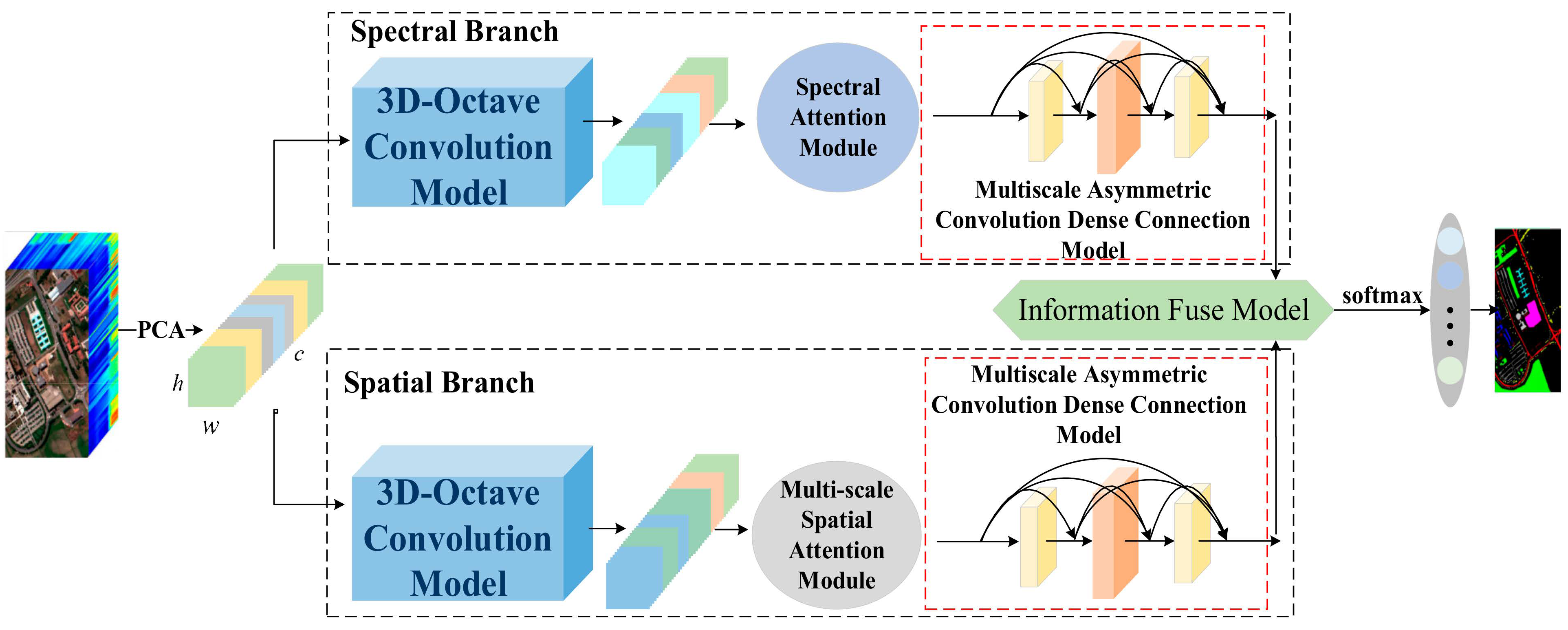
A double-branch structure is adopted in the proposed method, i.e., spectral information is obtained by the spectral branch, and spatial information is obtained by the spatial branch. First, the dimensionality of the hyperspectral image is reduced by principal component analysis (PCA). Next, the spectral information of the hyperspectral image is obtained from the spectral branch using the proposed 3D-OCONV. To fully capture spectral information, a spectral attention module and DC-TAC are used behind the 3D-OCONV. Then, to fully exploit the spatial features in the spatial branches, a combination of 3D-OCONV and 3D-MSSAM is used to improve the representation of spatial information, and DC-TAC is used to continue capturing spatial information. The overall schematic diagram of the proposed method is shown in Figure 1. Finally, through the above operations, two maps of spatial and spectral features are obtained. This paper designs an interactive information fusion module that can make full use of the information in these two parts. Through the information fusion module, spatial and spectral features can be fused by learning from each other, important information can be retained, and redundant information can be removed. Below, each module of the proposed method, i.e., 3D-OCONV, 3D-MSSAM, spectral attention module, DC-TAC, and interactive information fusion module, is introduced.

2.2. 3D-OCONV

For the network framework of hyperspectral image classification based on ordinary 3D-CNN, there is some spatial and spectral redundancy in the extracted feature map, which increases the storage and computing costs. Hyperspectral images contain abundant information. The purpose of using octave convolution is to halve the spatial resolution of low-frequency feature maps, reduce redundant spatial information, and improve the computational efficiency of the network. The original octave convolution [58] can process two-dimensional data effectively. A three-dimensional octave convolution is used in the network structure proposed in this paper. We replace the original two-dimensional average pooling with three-dimensional average pooling, set the size of the three-dimensional average pooling convolution kernel to (1, 1, 1), and set the stride to (1, 1, 1), so that more feature information on the extracted feature map can transmit to the next layer. In order to fully extract spatial and spectral information, all the two-dimensional convolutions in the octave convolution are replaced by three-dimensional convolutions. The size of the convolution kernel is set to (3, 3, 1), the stride is set to (1, 1, 1), and the padding is set to (1, 1, 0).

The use of three-dimensional octave convolution enables more efficient processing of hyperspectral image signatures and reduces channel redundancy through orthogonal and interactive methods.

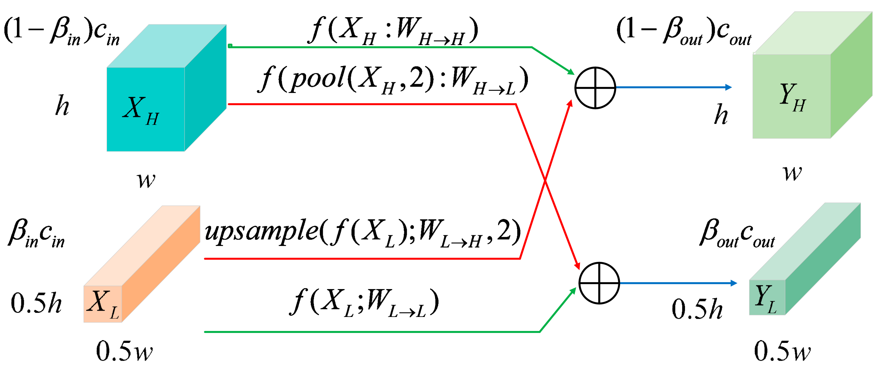
The structure of the 3D octave convolution is shown in Figure 2. It can be seen from Figure 2 that the 3D-OCONV consists of four paths. The information update of the high-frequency and low-frequency feature maps is indicated by the two green paths, and the information exchange between the two octaves is indicated by the two red paths. Suppose that $X\in P^{h\times w\times c}$ represents the input feature tensor of octave convolution, where $h$ and $w$ represent the spatial size, and $c$ represents the number of feature maps or channels. The input feature $X$ is decomposed into $X=\{X=X_H,X_L\}$ along the channel dimension, where $X_H\in P^{(1-\beta )h\times w\times c}$ represents the high-frequency feature map to capture image details, and $X_L\in P^{\beta \frac{h}{2}\times \frac{w}{2}\times c}$ represents the low-frequency feature map with more contextual information. $\beta \in [0,1]$ represents the channel ratio allocated to the high-frequency part, and the definition of the high-frequency feature map is eight degrees higher than that of the low-frequency part. This operation makes the spatial resolution of the input features different, and the traditional convolution cannot be represented in this way.

The low-frequency part $X_L$ is upsampled to the original spatial or spectral resolution, and then convoluted with the high-frequency part $X_H$. The low-frequency part is pooled to reduce the spatial or spectral resolution, and then connected with the low-frequency part for convolution. This not only enables the low-frequency information and high-frequency information in the tensor to be effectively processed but also enables effective inter-frequency communication. Let $Y$ be the output tensor; the high-frequency and low-frequency output feature maps are denoted by $Y=\{Y_H,Y_L\}$, where $Y_H=Y_{H\to H}+Y_{L\to H}$, $Y_L=Y_{L\to L}+Y_{H\to L}$, and $Y_{A\to B}$ represent the convolution update from group $A$ to group $B$ of the feature map, $Y_{H\to H}$ and $Y_{L\to L}$ represent the intra-frequency update, and $Y_{H\to L}$ and $Y_{L\to H}$ represent inter-frequency communication. The convolution kernel $W$ is divided into two components $W=\{W_H,W_L\}$, which are convoluted with $X_H$ and $X_L$, respectively. The two components of $W$ can be further divided into two parts, $W_H=[W_{H\to H},W_{L\to H}]$ and $W_L=[W_{L\to L},W_{H\to L}]$, as shown in Figure 3.

For the high-frequency feature map, regular convolution is used at position $(p,q)$. For inter-frequency communication, the low-frequency feature map is connected with the high-frequency feature after upsampling, and the process can be represented as follows:

$$\begin{array}{l}{Y}_H^{p,q}=Y_{H\to H}^{p,q}+Y_{L\to H}^{p,q}\\ ={{\displaystyle \sum _{i,j\in N_k}{W}_{H\to H}^{i+\raisebox{1ex}{$k-1$}\!\left/ \!\raisebox{-1ex}{$2$}\right.,j+\raisebox{1ex}{$k-1$}\!\left/ \!\raisebox{-1ex}{$2$}\right.}}}^T{X}_H^{p+i,q+j}\\ +{{\displaystyle \sum _{i,j\in N_k}{W}_{L\to H}^{i+\raisebox{1ex}{$k-1$}\!\left/ \!\raisebox{-1ex}{$2$}\right.,j+\raisebox{1ex}{$k-1$}\!\left/ \!\raisebox{-1ex}{$2$}\right.}}}^T{X}_L^{\left|\frac{p}{2}\right|+i,\left|\frac{q}{2}\right|+j}\end{array}$$

(1)

For the low-frequency feature map, in order to realize inter-frequency communication, the high-frequency features can be downsampled and then combined with the low-frequency feature map for convolution. The specific process is

$$\begin{array}{l}{Y}_L^{p,q}=Y_{L\to L}^{p,q}+Y_{H\to L}^{p,q}\\ ={{\displaystyle \sum _{i,j\in N_k}{W}_{L\to L}^{i+\raisebox{1ex}{$k-1$}\!\left/ \!\raisebox{-1ex}{$2$}\right.,j+\raisebox{1ex}{$k-1$}\!\left/ \!\raisebox{-1ex}{$2$}\right.}}}^T{X}_L^{p+i,q+j}\\ +{{\displaystyle \sum _{i,j\in N_k}{W}_{H\to L}^{i+\raisebox{1ex}{$k-1$}\!\left/ \!\raisebox{-1ex}{$2$}\right.,j+\raisebox{1ex}{$k-1$}\!\left/ \!\raisebox{-1ex}{$2$}\right.}}}^T{X}_H^{(2\times p+0.5+i),(2\times q+0.5+j)}\end{array}$$

(2)

where $(p,q)$ represents the position coordinate, and $N_K=\{(i,j):i=\{-\frac{k-1}{2},\dots ,\frac{k-1}{2}\},j=\{-\frac{k-1}{2},\dots ,\frac{k-1}{2}\left\}\right\}$ represents a local neighborhood. Each sample of position $\left(p,q\right)$ is multiplied by 2 before downsampling, and the position is further moved by half so that the downsampled feature map can be better aligned with the input spectral and spatial feature map. The convolution of low-frequency feature map $X_L$ and $k\times k\times n$ convolution kernel can effectively expand the receptive field twofold compared with ordinary convolution. Therefore, each layer can capture more context information and improve classification performance. When integrating high-frequency information and low-frequency information, in order to avoid errors in integrating different frequency information, average pooling is adopted for downsampling. The output $Y=\{Y_H,Y_L\}$ of octave convolution is

$$Y_H=f(X_H;W^{H\to H})+\mathit{upsample}(f(X_L;W_{L\to H}),2),$$

(3)

$$Y_L=f(X_{L;};W_{L\to L})+f(\mathit{pool}(X_H,2);W_{H\to L}),$$

(4)

where $f(X;W)$ represents the convolution with parameter $W$, $\mathit{pool}(X,k)$ represents the average pooling operation with kernel size $k\times k$ and step $k$, and $\mathit{upsample}(X,k)$ represents the upsampling operation with nearest interpolation factor $k$.

2.3. 3D-MSSAM

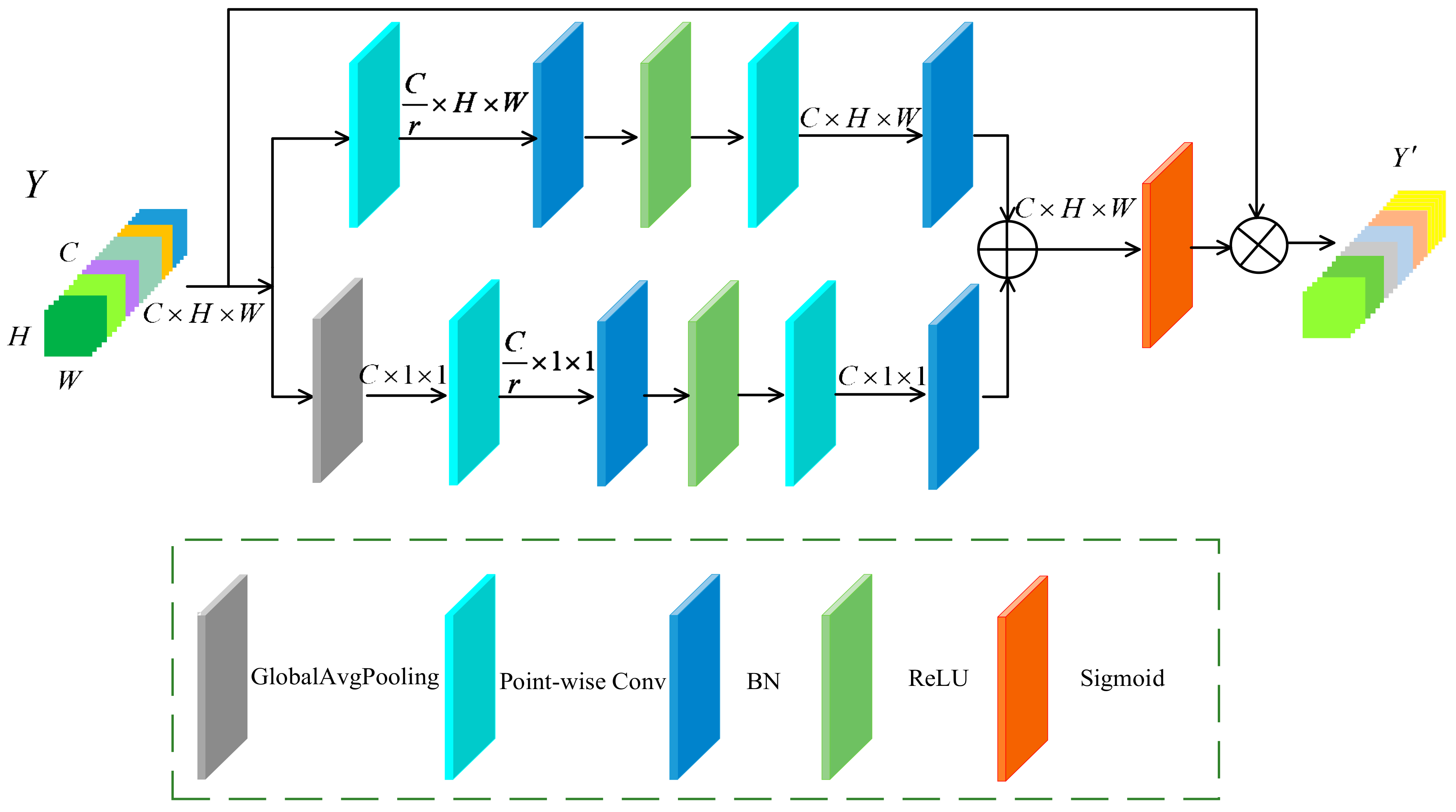
There is abundant spectral/spatial information contained in hyperspectral images. If this information can be fully extracted, the classification performance of hyperspectral images can be greatly improved. At present, linear operations are mainly used for feature fusion, such as summation or concatenation, but there are better choices. In [59], a multiscale channel attention module was used to extract important channel information through branches of different scales, such that features with inconsistent semantics and scales could be better integrated, and the problem of fusing features of different scales could also be solved. However, this module is only suitable for processing two-dimensional information. Abundant spectral/spatial information exists in hyperspectral images; thus, the multiscale channel attention module can be converted into a 3D-MSSA suitable for processing hyperspectral data. Figure 4 is a schematic diagram of 3D-MSSA.

The 3D-MSSAM uses 3D multiscale convolution to obtain the spatial information of hyperspectral images. The spatial attention $L(X)$ for extracting local features through multiscale three-dimensional convolution is

$$L(X)=B({\mathit{PWConv}}_2(\delta (B({\mathit{PWConv}}_1(x))))),$$

(5)

where ${\mathit{PWConv}}_1$ reduces the number of input feature channels of $X$ to the original $\frac{1}{r}$,$B$ represents the batchnorm layer, $\delta$ represents the ReLU activation function, ${\mathit{PWConv}}_2$ changes the number of channels to the same number as the original input channels through point convolution, and $r$ is the channel scaling ratio. The difference between the global feature channel attention $g(X)$ and $L(X)$ is that global average pooling (GAP) is performed on the input first. The output $X^{\prime }$ is

$$X^{\prime }=X\otimes M(X)=X\otimes \sigma (L(X)\oplus g(X)),$$

(6)

where $\sigma$ represents the sigmoid activation function, $\oplus$ represents the addition of input features, and $\otimes$ indicates that the corresponding elements of the feature map are multiplied.

2.4. Spectral Attention Module

Using the spectral attention module, the interdependencies between spectral feature maps can be mined, the highly dependent feature maps can be fully extracted, and the feature representation of semantic information can be effectively improved. In Figure 5, $U\in {ℝ}^{c\times p\times p}$ represents the spectral features, which are the initial input of the spectral attention module. Here, $p\times p$ is the input patch size, and $c$ represents the number of input channels. $Y$ is the spectral attention map, and the size of $Y$ is $c\times c$. $Y$ is calculated from the initial spectral feature maps $U$. $y_{\mathit{ij}}$ is used to measure the influence of the $i$-th spectral feature on the $j$-th spectral feature. $U_i$ is the $i$-th spectral feature, and $U_j$ is the $j$-th spectral feature. The calculation process is

$$y_{\mathit{ij}}=\frac{\exp (U_i\times U_j)}{{\displaystyle {\sum }_{i=1}^C\exp (U_i\times U_j)}}.$$

(7)

Then, the results of matrix multiplication between $Y$ and $U$ are reshaped into ${ℝ}^{c\times p\times p}$. Finally, the results are weighted by the scale $\alpha$ parameter, and input $U$ is added to obtain the final spectral attention map $E\in {ℝ}^{c\times p\times p}$ as follows:

$$E_j=\alpha {\displaystyle {\sum }_{i=1}^C(y_{\mathit{ij}}{U}_j)+U_j}.$$

(8)

Here, $\alpha$ is set to zero during initialization so that it can be learned gradually. The final map $E$ can improve the resolution of features because it includes the weighted sum of all channel features.

2.5. DC-TAC

For the convolution layer featuring a convolution kernel of size $(H\times W\times D)$, with the number of filters $C$ and $M$ channels as the input, $F\in R^{H\times W\times D}$ is used to represent the three-dimensional convolution kernel of the filter. For input $I\in R^{A\times B\times M}$, the input feature map has size $A\times B$ and channel number $M$. $O\in R^{S\times P\times C}$ represents the output of channel C. Thus, the corresponding output feature of the $j$ filter is

$$O:,:,j={\displaystyle \sum _{k=1}^M{I}_{:,:,k}\times F_{:,:,k}^{\left(j\right)}},$$

(9)

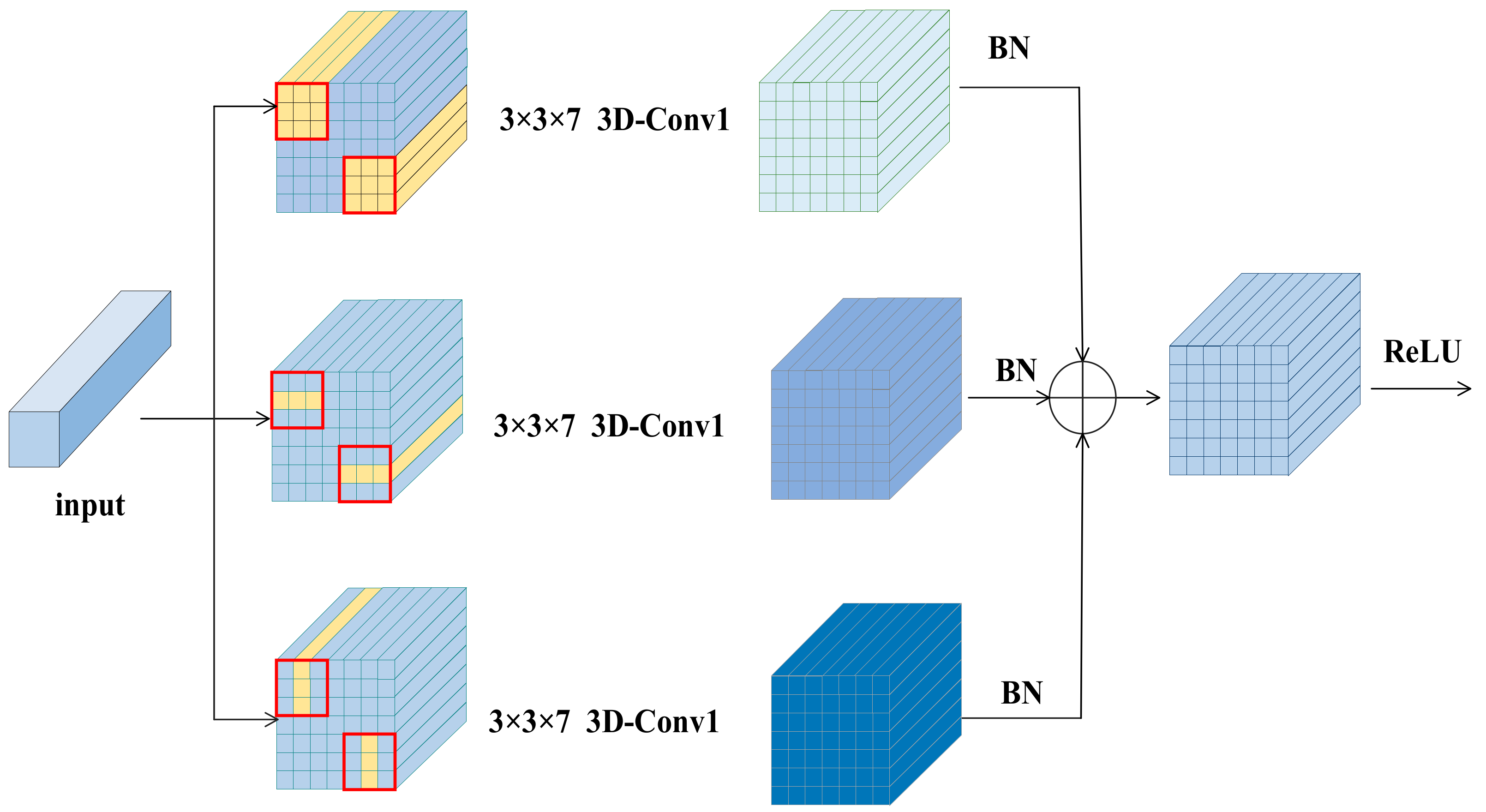
where $\times$ represents the three-dimensional convolution operator, $I_{:,:,k}$ is the $k$ channel with the spatial size $A\times B$ of the input feature map, and $k$ in $F_{:,:,k}^{(j)}$ is the $k$ input channel of $F^{(j)}$. In order to extract spatial feature information more effectively, using the idea of symmetric convolution, the convolution featuring a convolution kernel of size $(d\times d\times r)$ is constructed as an asymmetric convolution containing three parallel branches. The convolution kernels of the three branches are asymmetric convolution combinations with the sizes of $(d\times d\times r)$, $(d\times 1\times r)$, and $(1\times d\times r)$, as shown in the schematic diagram of asymmetric convolution in Figure 6. Let the input of the three branches of each group of asymmetric convolution be the same, let the step be the same, and let the upper left corner and upper right corner of the input cube data use the same sliding window. Using the additivity of the convolution, the outputs of the three branches are added to enrich the feature space. After the three branches are added, they are normalized, activated, and transported to the next set of asymmetric convolutions. In convolutional neural networks, batch normalization is widely used, which can effectively reduce overfitting and training time. The output feature maps after batch normalization are as follows:

$$O:,:,j=({\displaystyle \sum _{k=1}^M{I}_{:,:,k}\ast F_{:,:,k}^{(j)}F}-{\lambda }_j)\frac{{\alpha }_j}{{\delta }_j}+{\varphi }_j,$$

(10)

where ${\lambda }_j$ and ${\delta }_j$ are the mean and standard deviation of batch normalization, and ${\alpha }_j$ and ${\varphi }_j$ are the scale factor and offset, respectively. The output feature maps after convolution on each branch of each group of asymmetric convolution are fused together after BN normalization. For each filter $j$, let ${F^{\prime }}^{(j)}$ be the fused three-dimensional convolution kernel and ${\varphi }_j^{\prime }$ be the offset term obtained after fusion. The convolution kernels are $(1\times 3\times 7)$ and $(3\times 1\times 7)$, the filter kernels are ${\overline{F}}^{(j)}$ and ${\widehat{F}}^{(j)}$, and the bias terms are $\overline{\varphi }$ and ${\widehat{\varphi }}_j$, respectively. The convolution kernel with size $(3\times 3\times 7)$ is $F^{(j)}$, and the bias term is ${\varphi }_j$. Using the additivity of convolution, ${F^{\prime }}^{(j)}$ and ${\varphi }_j^{\prime }$ can be represented as

$${F^{\prime }}^{(j)}=\frac{{\alpha }_j}{{\delta }_j}{F}^{(j)}\oplus \frac{{\overline{\alpha }}_j}{{\delta }_j}{\overline{F}}^{(j)}\oplus \frac{{\widehat{\alpha }}_j}{{\delta }_j}{\widehat{F}}^{(j)},$$

(11)

$${\varphi }_j^{\prime }=-\frac{{\lambda }_j{\alpha }_j}{{\delta }_j}-\frac{{\overline{\lambda }}_j{\overline{\alpha }}_j}{{\delta }_j}-\frac{{\widehat{\lambda }}_j{\widehat{\alpha }}_j}{{\delta }_j}+{\varphi }_j+{\overline{\varphi }}_j+{\widehat{\varphi }}_j.$$

(12)

This additive property of the convolution kernel enables the transformed module to have the same output as the pre-transformed module, which significantly improves classification performance and accuracy without introducing additional parameters.

2.6. Interactive Information Fusion Module

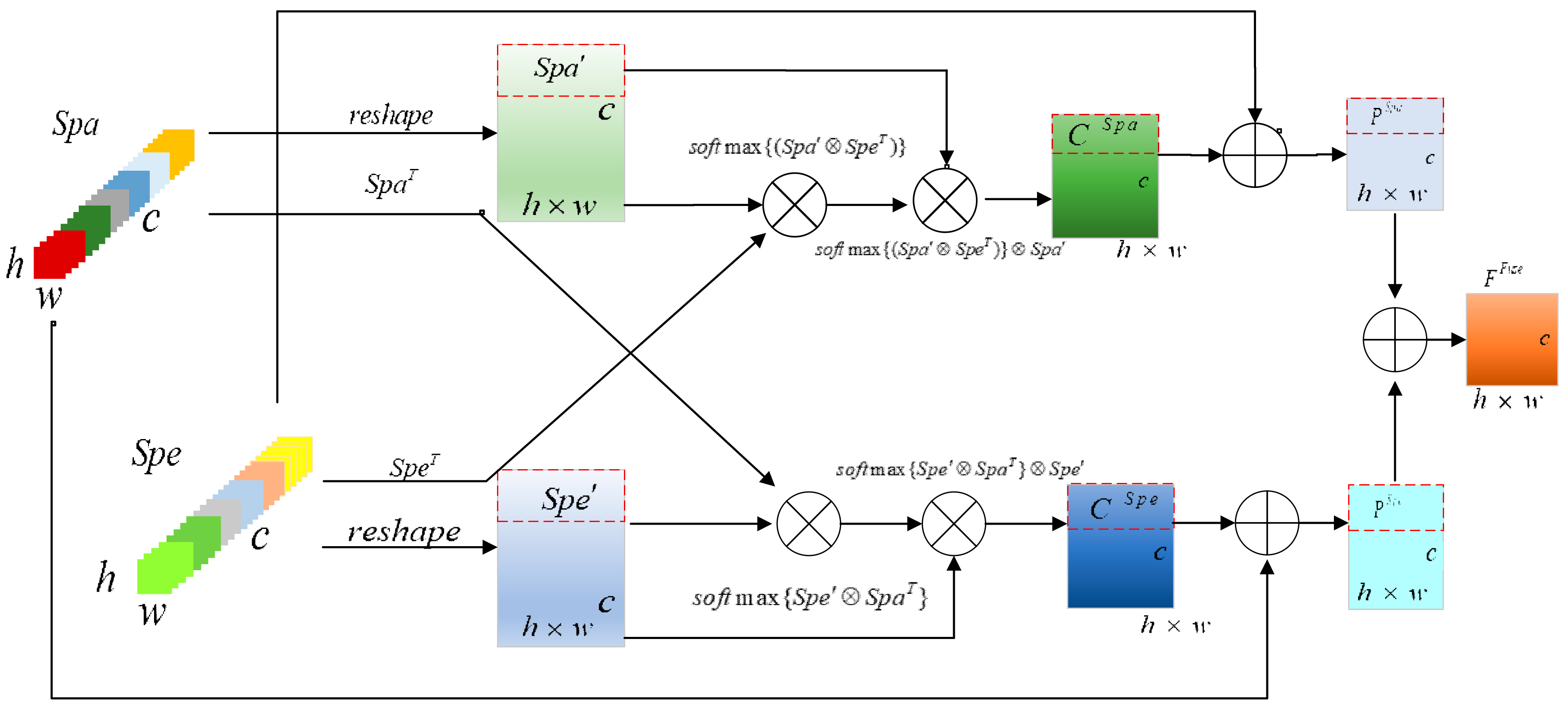
In this paper, a double-branch structure is adopted. However, it should be noted that the extracted spatial features also contain supplementary spectral information $C^{\mathit{Spatial}}$. Similarly, the extracted spectral features also contain supplementary spatial information $C^{\mathit{Spectral}}$. Finally, $C^{\mathit{Spatial}}$ and $C^{\mathit{Spectral}}$ are fused and then classified. The experimental results show that classification using fused spectral and spatial features can achieve better classification performance and higher classification accuracy than hyperspectral image classification using spatial or spectral features. A schematic diagram of the proposed interactive information fusion module is shown in Figure 7. For the convenience of calculation, firstly, the shape of the spatial feature is changed to ${\mathit{Spatial}}^{\prime }$, and the shape of the spectral feature is changed to ${\mathit{Spectral}}^{\prime }$. The spatial and spectral features are transposed to ${\mathit{Spatial}}^T$ and ${\mathit{Spectral}}^T$, respectively. The spatial and spectral features of transposition and shape change are used to obtain supplementary spatial features and supplementary spectral features. The specific formulas are as follows:

$$C^{\mathit{Spectral}}=\{\mathit{soft}\max ({\mathit{Spatial}}^{\prime }\otimes {\mathit{Spectral}}^T)\}\otimes {\mathit{Spatial}}^{\prime },$$

(13)

$$C^{\mathit{Spatial}}=\{\mathit{soft}\max ({\mathit{Spectral}}^{\prime }\otimes {\mathit{Spatial}}^T)\}\otimes {\mathit{Spectral}}^{\prime },$$

(14)

where $C^{\mathit{Spectral}}$ represents the transmission information from spatial features to spectral features, and $C^{\mathit{Spatial}}$ represents the transmission information from spectral features to spatial features. $\mathit{soft}\max ({\mathit{Spatial}}^{\prime }\otimes {\mathit{Spectral}}^T)$ represents the spatial supplementary information from spatial features to spectral features. By multiplying $\mathit{soft}\max ({\mathit{Spatial}}^{\prime }\otimes {\mathit{Spectral}}^T)$ and ${\mathit{Spatial}}^{\prime }$, the transmission information $C^{\mathit{Spectral}}$ from spatial information to spectral information can be obtained. $\mathit{soft}\max ({\mathit{Spectral}}^{\prime }\otimes {\mathit{Spatial}}^T)$ represents the spectral supplementary information from spectral features to spatial features. By multiplying $\mathit{soft}\max ({\mathit{Spectral}}^{\prime }\otimes {\mathit{Spatial}}^T)$ and ${\mathit{Spectral}}^{\prime }$, the transmission information $C^{\mathit{Spatial}}$ from spectral information to spatial information can be obtained.

In order to fuse spatial information into spectral features, $C^{\mathit{Spatial}}$ and $\mathit{Spectral}$ are added to obtain $P^{\mathit{Spatial}}$. In order to fuse spectral information into spatial information, $C^{\mathit{Spectral}}$ and $\mathit{Spatial}$ are added to obtain $P^{\mathit{Spectral}}$. The calculation formulas are as follows:

$$P^{\mathit{Spatial}}=C^{\mathit{Spatial}}+\mathit{Spectral},$$

(15)

$$P^{\mathit{Spectral}}=C^{\mathit{Spectral}}+\mathit{Spatial}.$$

(16)

Lastly, $P^{\mathit{Spatial}}$ and $P^{\mathit{Spectral}}$ are added to obtain the fused spatial/spectral information. The calculation formula is as follows:

$$F^{\mathit{Fuse}}=P^{\mathit{Spatial}}+P^{\mathit{Spectral}}.$$

(17)

3. Experiment

3.1. Datasets

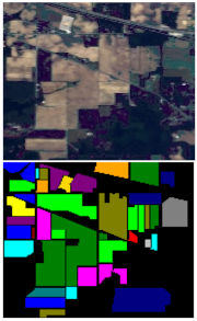
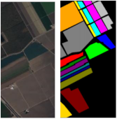
The four datasets used in the experiment, as well as the true image and false color image of the four datasets and the corresponding category information, are shown in

Table 1. Real image, false color map, and number of samples available in the Indian pines (IN) dataset.

Real Image and False Color Map	No.	Color	Name	Training	Test
	C1		Alfalfa	3	43
	C2		Corn-notill	42	1386
	C3		Corn-mintill	24	806
	C4		Corn	7	230
	C5		Grass-pasture	14	469
	C6		Grass-tress	21	709
	C7		Grass-pasture-mowed	3	25
	C8		Hay-windrowed	14	464
	C9		Oats	3	17
	C10		Soybean-notill	29	943
	C11		Soybean-mintill	73	2382
	C12		Soybean-clean	17	576
	C13		Wheat	6	199
	C14		Woods	37	1228
	C15		Buildings-grass-trees-drives	11	375
	C16		Stone-steel-towers	3	90
			Total	307	9942

,

Table 2. Real image, false color map, and number of samples available in the Pavia University (UP) dataset.

Real Image and False Color Map	NO.	Color	Name	Training	Test
	C1		Asphalt	33	6598
	C2		Meadows	93	18,556
	C3		Gravel	10	2089
	C4		Trees	15	3049
	C5		Painted metal sheets	6	1339
	C6		Bare soil	25	5004
	C7		Bitumen	6	1324
	C8		Self-modulating bricks	18	3664
	C9		Shadows	4	943
			Total	210	42,566

,

Table 3. Real image, false color map, and number of samples available in the Kennedy Space Center (KSC) dataset.

Real Image and False Color Map	NO.	Color	Name	Training	Test
	C1		Scrub	38	723
	C2		Willow swamp	12	231
	C3		CP hammock	12	244
	C4		Slash pine	12	240
	C5		Oak/broadleaf	8	153
	C6		Hard wood	11	218
	C7		Swamp	5	100
	C8		Graminoid marsh	21	410
	C9		Spartina marsh	26	494
	C10		Cattail marsh	20	384
	C11		Salt marsh	20	399
	C12		Mud flats	25	478
	C13		Water	46	881
			Total	256	4955

and

Table 4. Real image, false color map, and number of samples available in the Salinas Valley (SV) dataset.

Real Image and False Color Map	NO.	Color	Name	Training	Test
	C1		Brocoli_green_weeds_1	10	1999
	C2		Brocoli_green_weeds_2	18	3708
	C3		Fallow	9	1967
	C4		Fallow_rough_plow	6	1388
	C5		Fallow_smooth	13	2665
	C6		Stubble	19	3940
	C7		Celery	17	3562
	C8		Graps_untrained	56	11,215
	C9		Soil_vinyard_develop	31	6172
	C10		Corn_cenesced_green_weed	16	3262
	C11		Lettuce_romaine_4wk	5	1063
	C12		Lettuce_romaine_5wk	9	1833
	C13		Lettuce_romaine_6wk	4	912
	C14		Lettuce_romaine_7wk	5	1065
	C15		Vinyard_untrained	36	7232
	C16		Vinyard_vertical_trellis	9	1798
			Total	263	53,886

.

(1)

Indian pines (IN): As shown in Table 1, this was the earliest experimental dataset used for hyperspectral image classification. In 1992, an Indian pine tree in Indiana was imaged using an aerial visible/infrared imaging spectrometer (AVIRIS). The researchers used 145 size markers to perform hyperspectral image classification experiments. An image with a spatial resolution of about 20 m was generated by a spectral imager. To facilitate the experiment, 200 bands were left for the experiment, and the remaining unnecessary bands were eliminated. In the dataset, the number of pixels is 21,025, the number of ground objects is 10,249, and the number of background pixels is 10,776. There are 16 categories in the image with uneven distribution.

(2)

Pavia University (UP): The UP dataset is shown in Table 2. The UP dataset is part of the hyperspectral data from the German Airborne Reflective Optical System Imaging Spectrometer (ROSIS), which was used in 2003 to image the city of Pavia in Pavia, Italy. The spectral imager mapped 115 bands, eliminating 12 affected by noise and leaving 103 available bands. There are nine trees, asphalt pavement, and bricks in the dataset.

(3)

Kennedy Space Center (KSC): As shown in Table 3, the KSC dataset was collected on 23 March 1996 at the Kennedy Space Center in Florida by the NASA AVIRIS (Airborne Visible/Infrared Imaging Spectrometer) instrument. A total of 224 bands were collected. After removing the bands with water absorption and a low signal-to-noise ratio, 176 bands were left for analysis. There are 13 categories in the dataset representing various types of land cover in the environment.

(4)

Salinas Valley (SV): The SV dataset is shown in Table 4. The SV dataset comprised an image taken by an AVIRIS imaging spectrometer in Salinas Valley, California, USA. The SV dataset initially had 224 bands; after removing unnecessary bands, 204 bands remained for use. The size of the image is 512 × 217, and the number of pixels in the image is 111,104. After removing 56,975 background pixels, the remaining 54,129 pixels remained for classification. These pixels are classified into 16 categories, such as fallow cultivation and celery.

3.2. Experimental Setup and Evaluation Criteria

In the experiment, we set the learning rate to 0.0005. The hardware platform we used in the experiment was AMD Ryzen7 4800 h, with Radeon graphics 2.90 GHz, Nvida Geforce rtx2060 GPU, and 16 GB of memory. CUDA 10.0, pytorch 1.2.0, and python 3.7.4 were the software environments used for the experiments. For the module proposed in this paper, the input data size of different datasets was set to $O\in P^{9\times 9\times N}$, where N is the number of bands in the dataset. Furthermore, 3%, 0.5%, 0.4%, and 5% of the data were randomly selected from the IN, UP, KSC, and SV datasets, respectively. Randomly selected data were used as training samples for the experiment, while other data were used as test samples for the experiment.

Overall accuracy (OA), average accuracy (AA), and Kappa coefficients were used to comprehensively evaluate the proposed methods. Experiments were performed on four datasets: IN, UP, KSC, and SV. We set the number of experiment iterations to 200, the batch size to 16, and the number of repetitions per experiment to 10. Taking the average value of several groups of experimental results as the final result of the experiment effectively avoided the data deviation caused by randomness.

3.3. Experimental Results

In order to verify the effectiveness of the proposed method, 10 different methods were selected for comparison with the proposed method. These methods included traditional machine learning methods and methods based on deep learning. Methods based on deep learning included DBDA [49], SSRN [50], PyResnet [51], FDSSC [52], DBMA [53], A2S2KResNet [60], CDCNN [61], and HybridSN [62], and traditional machine learning methods included SVM [63]. The visual transformer (ViT) [64] model, which performs well in the field of image processing, is a classic model. In addition, for the sake of fairness, all comparison methods were carried out under the same conditions as the methods proposed in this paper, including experimental parameter setting and experimental data preprocessing.

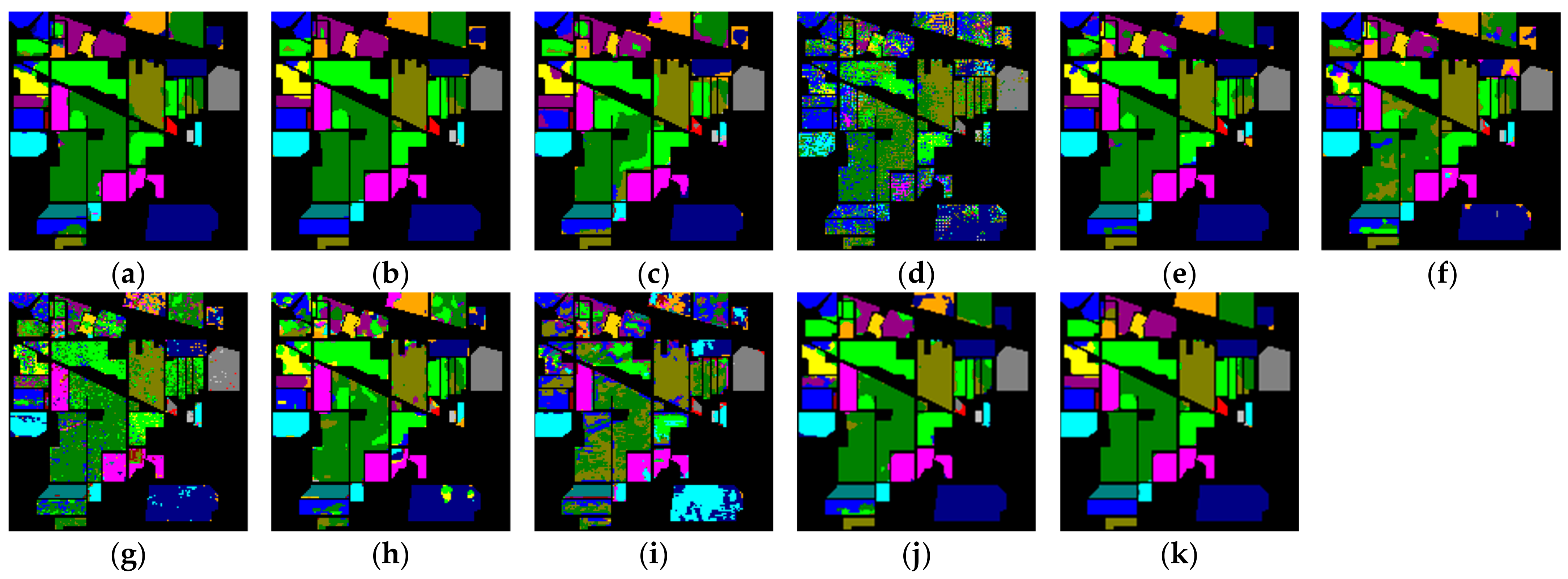
(1) Analysis of experimental results on the IN dataset: Figure 8 shows a visual classification diagram obtained using different methods on the data, and

Table 5. KPIs (OA, AA, and kappa) on the Indian pines (IN) dataset with 3% training samples.

Class	PyResNet	SVM	CDCNN	HybridSN	SSRN	ViT	DBMA	A2S2KResNet	FDSSC	DBDA	Proposed
C1	23.24	35.61	48.56	81.79	81.53	98.86	82.25	89.41	83.52	96.49	99.26
C2	59.25	56.48	66.86	69.12	88.18	73.71	85.93	90.48	90.44	92.25	96.65
C3	45.96	61.56	33.13	91	86.68	68.26	88.64	92.32	87.60	91.6	97.76
C4	34.77	41.55	54.91	84.87	83.27	81.69	87.99	93.78	91.24	92.63	97.22
C5	66.03	83.06	87.35	90.73	96.78	84.26	95.05	97.83	98.31	97.76	98.35
C6	73.15	84.34	91.16	88.59	95.44	84.16	97.53	97.20	98.25	96.85	99.04
C7	32.35	57.86	57.25	83.62	85.98	91.72	51.11	88.69	87.70	65.62	79.78
C8	89.90	88.68	92.92	87.24	95.75	91.95	98.62	98.80	98.45	98.75	99.82
C9	32.33	37.46	48.08	60.44	72.16	78.62	53.31	64.55	72.11	83.42	92.63
C10	50.51	63.33	64.95	86.25	84.93	75.44	86.22	88.58	83.95	86.47	90.85
C11	51.52	64.74	67.74	88.95	88.26	76.28	89.51	89.75	95.72	93.12	95.80
C12	54.67	51.56	41.31	79.03	85.34	67.03	83.18	92.48	90.50	91.22	95.27
C13	76.89	84.75	85.68	93.64	98.15	92.47	96.8	96.88	98.99	96.69	98.88
C14	72.50	89.68	87.25	92.65	94.53	91.89	96.52	96.02	95.95	96.15	97.22
C15	37.80	63.83	86.64	88.83	88.65	81.34	85.19	91.34	92.51	92.37	96.74
C16	68.35	97.67	91.43	92.23	94.48	83.51	95.47	93.60	98.01	90.83	90.21
OA (%)	51.03 ± 0.04	67.77 ± 0	71.42 ± 2.56	82.18 ± 1.5	89.24 ± 0.41	78.62	89.95 ± 1.06	92.10 ± 0.01	92.29 ± 2.56	92.58 ± 0.53	96.23 ± 0.01
AA (%)	54.32 ± 0.05	68.74 ± 0	71.35 ± 1.21	84.31 ± 1.61	88.69 ± 0.95	82.25	86.80 ± 0.59	91.36 ± 0.02	91.45 ± 2.56	91.17 ± 0.22	95.57 ± 0.85
Kappa (%)	43.21 ± 0.05	64.97 ± 0	67.22 ± 2.74	79.85 ± 1.42	87.88 ± 0.47	75.64	88.24 ± 1.19	90.96 ± 0.01	91.24 ± 2.56	91.6 ± 0.63	95.70 ± 0.90

shows the numerical classification results obtained using different methods on the dataset. By observing the classification results of each method, we can find that, compared with other comparative methods, the classification results of the method proposed in this paper were the clearest and closest to the ground-truth map. Not only was the classification result in the region good, but the classification result at the boundary of the region was also better than that of the other methods. By observing the numerical results in Table 5, it can be found that the proposed method had the best classification performance compared with other methods. Compared with other methods, the OA of the proposed method increased by 4.13% (A2S2KResNet), 3.65% (DBDA), 6.28% (DBMA), 45.2% (PyResNet), 6.99% (SSRN), 28.46% (SVM), 14.05% (HybridSN), 24.81% (CDCNN), 3.94% (FDSSC), and 17.61% (ViT). The AA increased by 4.21% (A2S2KResNet), 4.4% (DBDA), 8.77% (DBMA), 41.25% (PyResNet), respectively 6.88% (SSRN), 26.83% (SVM), 11.26% (HybridSN), 24.22% (CDCNN), 4.12% (FDSSC), and 13.32% (ViT), and kappa increased by 4.74% (A2S2KResNet), 4.1% (DBDA), 7.46% (DBMA), 52.49% (PyResNet), 7.82% (SSRN), 30.73% (SVM), 15.85% (HybridSN), 28.48% (CDCNN), 4.46% (FDSSC), and 20.06% (ViT). The experimental results showed that the classification performance of this method was better. Compared with other comparison methods, this method is more comprehensive in extracting the spectral and spatial features of hyperspectral images.

The experimental results showed that the classification performance of this method was better than that of other methods in most cases. For example, for C8 haystack, A2S2KResNet, and OA achieved the best classification among all comparison methods, while the OA for C8 haystack was 99.82%, which is higher than for all other methods. Combined with the above discussion of the experimental results, it is shown that the proposed method was effective for the IN dataset.

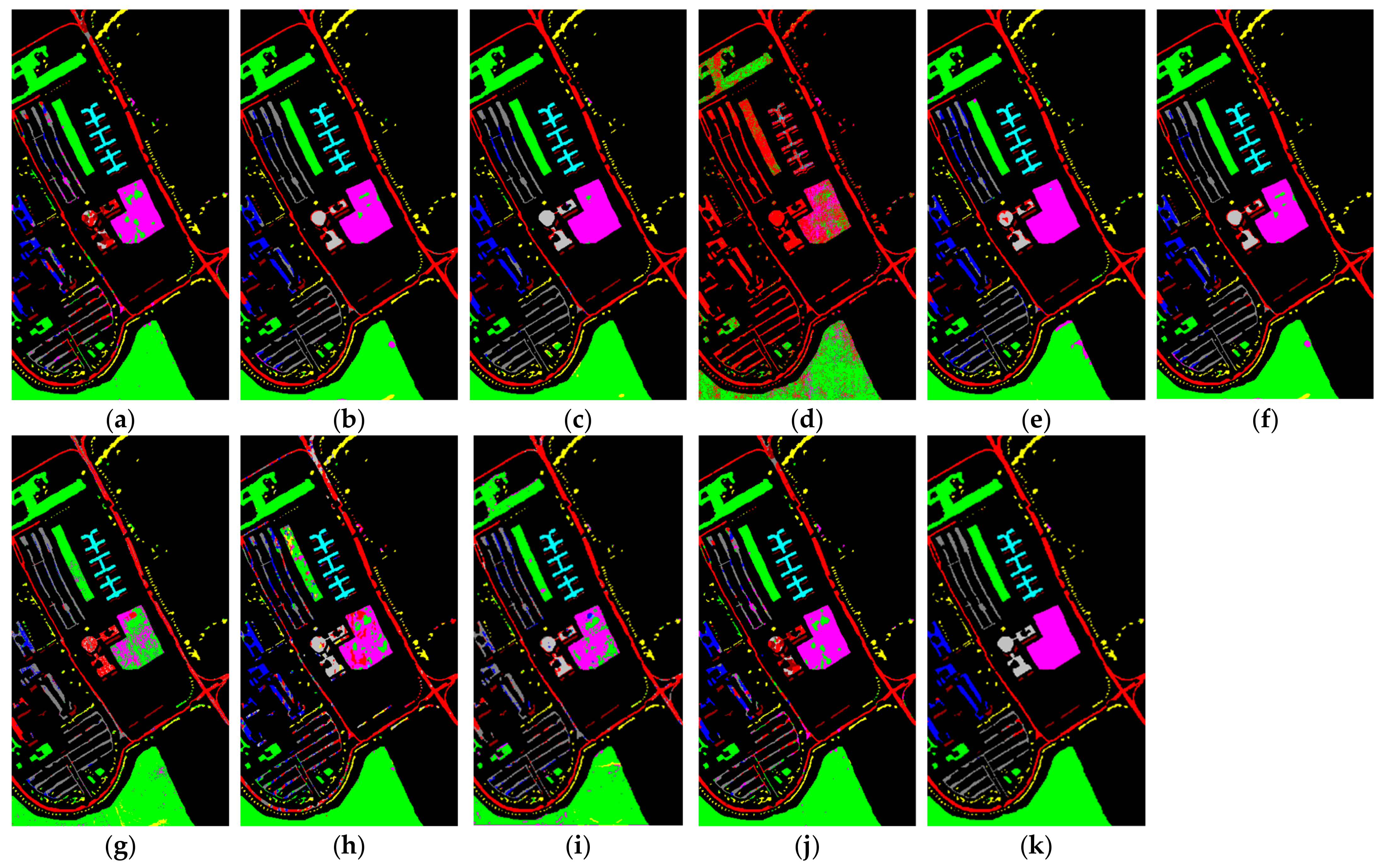
(2) Analysis of experimental results on the UP dataset: Figure 9 shows the visual classification diagrams obtained using different methods on UP data, and

Table 6. KPIs (OA, AA, and kappa) on the Pavia University (UP) dataset with 0.5% training samples.

Class	PyResNet	SVM	CDCNN	HybridSN	SSRN	ViT	DBMA	A2S2KResNet	FDSSC	DBDA	Proposed
C1	39.25	82.27	87.78	76.91	94.10	89.63	88.83	83.81	91.64	92.52	95.64
C2	71.05	83.54	94.73	92.80	96.66	96.46	97.07	92.72	97.06	98.07	99.30
C3	50.69	57.55	65.28	69.34	76.75	81.26	77.08	72.96	86.22	87.86	97.07
C4	65.45	93.33	96.13	80.84	99.29	98.03	96.71	98.11	96.75	96.27	98.38
C5	98.64	94.37	97.53	98.85	99.64	95.76	97.46	98.67	99.74	97.84	98.60
C6	44.86	81.66	89.62	83.48	93.85	93.32	93.66	86.51	96.83	98.47	98.97
C7	23.89	48.14	78.28	65.72	86.48	78.26	87.73	88.07	71.04	92.62	97.98
C8	27.76	72.15	78.53	55.59	83.71	88.48	81.17	74.10	77.84	87.43	87.74
C9	16.39	98.96	92.05	60.94	98.97	98.21	95.37	90.97	98.73	97.47	98.03
OA (%)	5464 ± 0.06	83.03 ± 0	87.94 ± 0.13	81.85 ± 0.01	92.50 ± 1.32	93.24 ± 1.06	91.8 ± 0.56	87.44 ± 0.02	93.16 ± 2.56	96.01 ± 0.03	97.26 ± 0.67
AA (%)	4867 ± 0.11	78.24 ± 0	85.32 ± 0.19	76.05 ± 0.03	92.16 ± 1.31	91.04 ± 1.13	90.01 ± 2.64	87.32 ± 0.02	90.58 ± 2.56	94.72 ± 0.59	96.85 ± 0.94
Kappa (%)	3532 ± 0.08	76.45 ± 0	83.95 ± 0.16	75.78 ± 0.02	90.89 ± 1.61	91.37 ± 1.01	89.04 ± 0.75	83.15 ± 0.02	90.88 ± 2.56	94.71 ± 0.04	96.37 ± 0.90

shows the numerical classification results obtained using different methods on the UP dataset. From the classification results shown in Figure 9, it can be seen that the classification results obtained using the proposed method were clearer and closer to the ground-truth map than those obtained using the other methods. By comparing the classification results of the proposed method with those of other methods, it was found that the proposed method could accurately predict almost all samples. At the same time, the classification results in Table 6 show that the proposed method had the best classification performance compared with all other comparison methods. The OA of the proposed method increased by 9.82% (A2S2KResNet), 1.25% (DBDA), 5.46% (DBMA), 42.62% (PyResNet), 4.76% (SSRN), 14.23% (SVM), 15.41% (HybridSN), 9.32% (CDCNN), 4.1% (FDSSC), and 3.99% (ViT). The AA of the proposed method increased by 9.53% (A2S2KResNet), 2.13% (DBDA), 6.84% (DBMA), 48.18% (PyResNet), 4.69% (SSRN), 18.61% (SVM), 20.8% (HybridSN), 11.53% (CDCNN), 6.27% (FDSSC), and 5.81% (ViT). The kappa of the proposed method increased by 13.22% (A2S2KResNet), 1.66% (DBDA), 7.33% (DBMA), 61.05% (PyResNet), 5.48% (SSRN), 19.92% (SVM), 20.59% (HybridSN), 12.42% (CDCNN), 5.49% (FDSSC), and 5% (ViT). A comprehensive analysis of the above classification results shows that the proposed method could effectively capture more useful classification features.

Compared with the other comparison methods, the proposed method had the highest accuracy for some categories in the UP dataset, such as C2 grassland and C6 bare soil, with the highest classification accuracy of 99.30% and 98.97%. For other categories, this method could also achieve high classification performance. In addition, for C7 asphalt, the classification accuracy of DBDA and DBMA with an attention mechanism was 92.62% and 87.73%, which was significantly higher than that of other methods, successfully proving that spatial attention and spectral attention play a positive role in feature learning. The proposed method had the best classification effect. In combination with the above comprehensive analysis, it can be proven that the proposed three-dimensional multiscale space attention module can extract more spatial features conducive to classification.

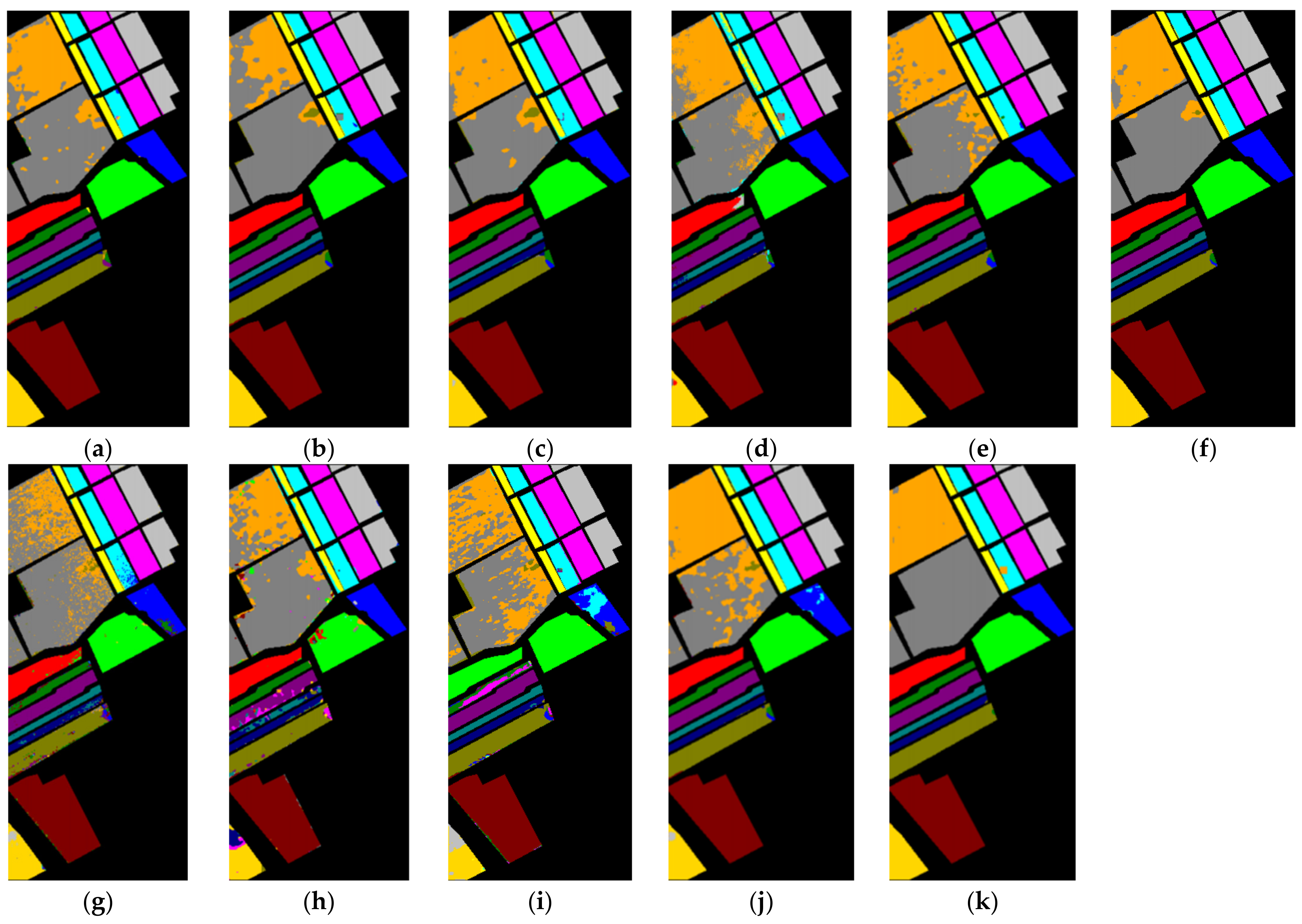
(3) Analysis of experimental results on SV dataset: Figure 10 shows the results of the visual classification of the SV dataset using different methods.

Table 7. KPIs (OA, AA, and kappa) on the Salinas Valley (SV) dataset with 0.5% training samples.

Class	PyResNet	SVM	CDCNN	HybridSN	SSRN	ViT	DBMA	A2S2KResNet	FDSSC	DBDA	Proposed
C1	98.49	99.41	97.75	84.65	96.17	96.76	97.53	99.83	100	98.74	99.22
C2	99.68	97.89	97.47	95.49	97.85	98.32	98.63	99.99	96.99	98.18	99.46
C3	96.36	88.99	88.54	88.10	95.26	96.41	95.82	94.97	98.01	96.48	97.63
C4	96.68	96.59	94.56	65.21	98.66	97.89	91.16	96.15	96.96	95.31	95.99
C5	91.02	96.08	95.09	91.03	97.25	97.55	95.75	99.13	99.58	97.15	99.76
C6	99.61	99.91	96.35	99.42	98.95	98.80	98.33	99.72	99.66	98.85	99.94
C7	98.68	96.62	93.88	97.16	98.33	96.72	96.69	99.72	92.07	99.33	97.75
C8	83.08	73.17	81.45	83.37	87.26	91.32	88.39	90.15	99.56	92.84	99.80
C9	98.85	97.09	97.59	98.95	99.37	93.27	98.16	99.66	97.03	98.06	95.92
C10	97.54	86.37	85.83	93.57	96.37	92.05	94.88	98.51	97.30	98.53	95.07
C11	95.31	86.97	83.66	54.51	96.82	93.07	92.63	95.20	96.06	96.74	99.24
C12	98.18	96.21	96.77	86.55	97.42	98.89	96.78	97.63	98.41	97.85	99.18
C13	75.11	92.45	97.87	44.36	97.24	97.43	97.28	97.09	99.90	98.48	99.91
C14	87.30	93.02	93.22	43.26	97.81	94.23	96.96	93.28	96.75	97.56	96.18
C15	81.14	76.02	73.85	86.07	84.33	82.98	84.03	84.79	86.87	84.23	87.07
C16	98.54	98.82	96.81	93.78	99.54	95.88	98.04	99.77	99.66	98.96	99.77
OA (%)	91.51 ± 0.01	86.98 ± 0	88.36 ± 0.28	87.33 ± 0.04	92.04 ± 0.96	95.79 ± 0.53	92.95 ± 0.33	94.58 ± 0.01	95.79 ± 0.36	93.74 ± 0.74	97.34 ± 0.01
AA (%)	93.47 ± 0.02	91.56 ± 0	91.95 ± 0.66	81.59 ± 0.12	95.95 ± 0.21	94.43 ± 0.62	95.68 ± 0.2	96.60 ± 0.01	97.50 ± 0.54	96.76 ± 0.17	97.91 ± 0.28
Kappa (%)	90.54 ± 0.01	85.45 ± 0	87.05 ± 0.3	85.89 ± 0.05	91.14 ± 1.08	95.45 ± 0.69	92.16 ± 0.34	93.97 ± 0.01	95.31 ± 0.32	93.05 ± 0.8	97.04 ± 0.01

shows the numerical classification results for the SV dataset using different methods. By looking at Figure 10, we can see that the classification map of the proposed method was closer to the ground-truth map than the other methods. The classification boundaries of the different categories were also very clear, and almost all samples could be accurately predicted. By looking at Figure 10, it can be found that the proposed method had the best classification effect compared with other methods. The OA of the proposed method increased by 2.76% (A2S2KResNet), 3.6% (DBDA), 4.39% (DBMA), 5.83% (PyResNet), 5.3% (SSRN), 10.36% (SVM), 10.01% (HybridSN), 8.98% (CDCNN), 1.55% (FDSSC), and 4.96% (ViT); the AA increased by 1.31% (A2S2KResNet) 1.15% (DBDA), 2.23% (DBMA), 4.44% (PyResNet), 1.96% (SSRN), 6.35% (SVM), 16.32% (HybridSN), 5.96% (CDCNN), 0.41% (FDSSC) and 3.48% (ViT); and kappa increased by 3.07% (A2S2KResNet), 4.01% (DBDA), 4.88% (DBMA), 6.5% (PyResNet), 5.9% (SSRN), 11.59% (SVM), 11.15% (HybridSN), 9.99% (CDCNN), 1.73% (FDSSC) and 1.59% (ViT). Combined with the above analysis of the classification results, we found that the proposed method had better classification results.

The classification accuracy of C6 stubble and C13 lettuce reached 99.94% and 99.91%, respectively. According to the above analysis and the classification results in the SV dataset, the classification performance of the proposed method was better than that of the other methods.

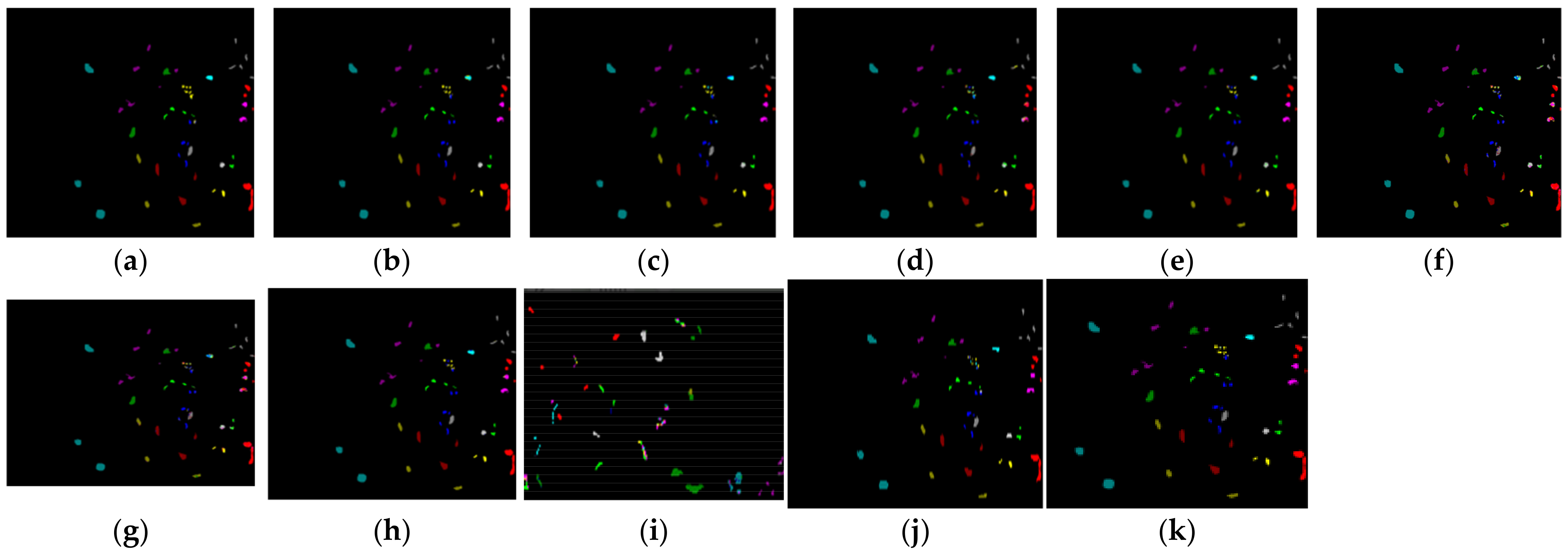
(4) Analysis of experimental results on the KSC dataset: Figure 11 shows the visual classification maps obtained using different methods on KSC datasets, and

Table 8. KPIs (OA, AA, and kappa) on the Kennedy Space Center (KSC) dataset with 5% training samples.

Class	PyResNet	SVM	CDCNN	HybridSN	SSRN	ViT	DBMA	A2S2KResNet	FDSSC	DBDA	Proposed
C1	94.09	92.43	96.81	88.08	98.4	89.06	99.39	98.28	99.73	99.67	99.51
C2	85.59	87.14	83.65	76.94	94.52	92.79	93.8	96.06	93.99	95.08	96.13
C3	81.14	72.47	83.92	69.65	85.2	91.82	80.2	92.01	82.50	88.72	92.16
C4	77.23	54.45	58.61	71.36	74.55	90.62	75.31	87.51	78.78	80.82	89.55
C5	74.96	64.11	52.83	83.99	75.13	90.29	69.6	86.26	68.55	78.14	91.87
C6	78.76	65.23	77.17	73.62	94.35	96.01	95.06	100	93.31	97.75	99.30
C7	84.73	75.5	75.34	63.61	84.64	92.43	87.08	88.30	88.69	95.15	95.58
C8	95.21	87.33	85.83	76.35	96.97	88.50	95.4	89.30	98.83	99.08	99.11
C9	93.93	87.94	91.65	74.55	97.83	90.74	96.21	100	99.80	99.98	100
C10	98.96	96.01	93.87	80.07	98.84	83.98	96.13	98.87	100	99.92	99.95
C11	99.48	96.03	98.77	94.41	99.14	93.15	99.64	98.82	99.15	98.92	99.33
C12	96.13	93.75	94.08	71.55	98.17	86.79	98.19	96.73	98.07	97.95	98.48
C13	99.72	99.72	99.8	91.96	100	95.64	100	100	100	99.97	99.94
OA (%)	91.49 ± 0.02	87.96 ± 0	89.33 ± 0.65	79.72 ± 4.31	94.52 ± 0.9	92.38 ± 0.16	94.12 ± 0.27	91.22 ± 0.58	95.62 ± 0.03	96.76 ± 0.51	98.89 ± 0.45
AA (%)	89.23 ± 0.02	82.55 ± 0	84.03 ± 0.95	78.17 ± 4.24	92.15 ± 1.87	93.67 ± 0.09	91.23 ± 0.75	90.76 ± 0.49	92.49 ± 0.06	94.9 ± 0.2	98.33 ± 0.19
Kappa (%)	90.52 ± 0.02	86.59 ± 0	88.13 ± 0.73	77.43 ± 4.7	93.9 ± 1	91.85 ± 0.12	93.45 ± 0.31	92.14 ± 0.59	95.12 ± 0.03	96.4 ± 0.57	98.65 ± 0.36

shows the numerical classification results obtained using different methods on KSC datasets. As can be seen from the classification result diagram shown in Figure 11, the classification results of the proposed method were the clearest. Specifically, the OA of the proposed method increased by 7.67% (A2S2KResNet), 2.13% (DBDA), 4.77% (DBMA), 7.4% (PyResNet), 4.37% (SSRN), 10.93% (SVM), 19.17% (HybridSN), 9.56% (CDCNN), 3.27% (FDSSC), and 6.51% (ViT); AA increased by 7.57% (A2S2KResNet) 3.43% (DBDA), 7.1% (DBMA), 9.1% (PyResNet), 6.18% (SSRN), 15.78% (SVM), 20.15% (HybridSN), 14.3% (CDCNN), 5.84% (FDSSC) and 4.66% (ViT); and kappa increased by 6.51% (A2S2KResNet), 2.25% (DBDA), 5.2% (DBMA), 8.13% (PyResNet), 4.75% (SSRN), 12.06% (SVM), 21.22% (HybridSN), 10.52% (CDCNN), 3.53% (FDSSC) and 6.8% (ViT). By observing the experimental results, it was found that the method could extract more features that contributed to the classification.

By observing the classification results of different categories in the KSC dataset, it is clear that, in most cases, the classification performance of the proposed method was better than that of other comparison methods. For example, the classification accuracy of C8 grass swamp and C9 rice grass swamp reached 99.11% and 100%, respectively. According to the above comprehensive analysis, the classification performance of this method was better than that of other methods.

4. Discussion

4.1. The Performance Analysis of Each Module

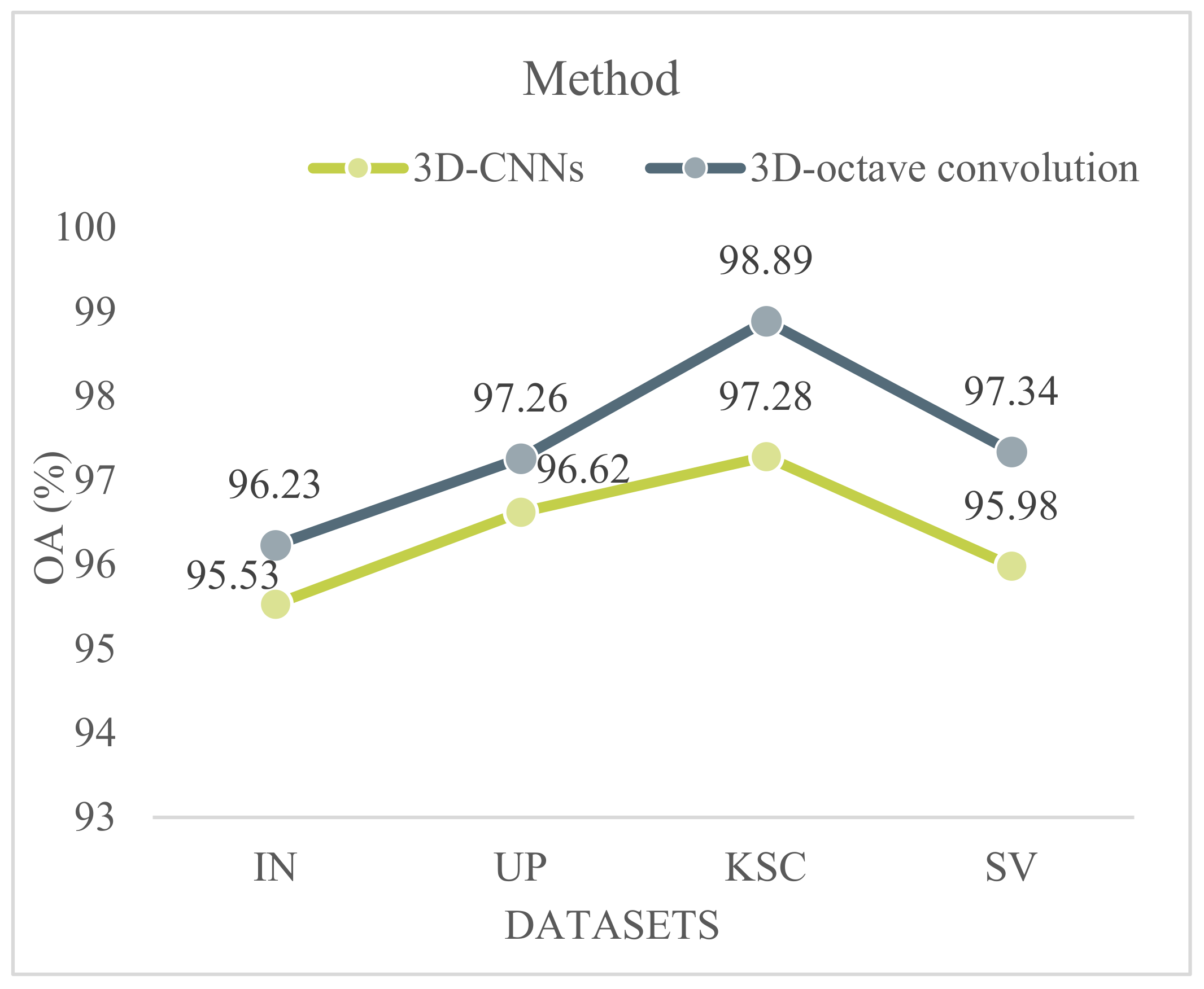
(1) 3D-OCONV: In order to verify that the 3D-OCONV used in the proposed method could effectively improve classification performance, this paper presents a comparative experiment using 3D-CNNs instead of 3D-OCONV (proposed method) to extract the spatial and spectral information of hyperspectral images. Experiments were carried out on four datasets: IN, UP, KSC, and SV. Figure 12 shows the OAs of the 3D-CNNs and 3D-OCONV. By looking at Figure 12, it is clear that the OA of the proposed method was the highest. The OA of the proposed method on the four datasets (IN, UP, KSC, and SV) was 0.7%, 0.64%, 1.61%, and 1.36% higher compared to 3D-CNNs, respectively. This demonstrates that the features extracted by 3D-OCONV were more representative and comprehensive, thus achieving good classification performance for hyperspectral images.

(2) 3D-MSSAM: Five groups of modules were designed and compared with the proposed 3D-MSSAM to verify classification performance. The first set of modules did not use spectral attention or multiscale spatial attention, recorded as “no attention.” The second group of modules only used spectral attention, recorded as “spectral attention.” The third group of modules only used spatial attention, recorded as “spatial attention.” The fourth group of modules only used 3D-MSSAM, recorded as “3D-MSSAM.” The fifth group of modules adopted both spectral attention and spatial attention, recorded as “spectral + spatial attention.” The sixth group of modules included all modules proposed in this paper, recorded as the “proposed method.” For a fair comparison, the components were evaluated under the same conditions. The comparative experiments of the six groups of modules were carried out on four datasets: IN, UP, KSC, and SV.

Table 9. The OAs of different feature extraction modules on IN, UP, KSC, and SV datasets (%).

	No Attention	Spectral Attention	Spatial Attention	3D-MSSAM	Spectral + Spatial Attenton	Proposed Method
IN	95.20	94.88	95.40	96.11	94.07	96.23
UP	94.82	95.23	94.28	95.16	96.36	97.26
KSC	97.82	97.74	97.70	96.85	96.46	98.89
SV	96.32	96.08	96.25	96.15	96.03	97.34

shows the OAs of the six modules for the different datasets. By observing Table 9, we can find that the OA value of the proposed method was the highest. Compared with other modules, on the IN dataset, the OA of the proposed module was 1.03%, 1.35%, 0.83%, 0.12%, and 2.16% higher compared to “no attention,” “spectral attention,” “spatial attention,” “3D-MSSAM,” and “spectral + spatial attention,” respectively. In the UP dataset, the OA of the proposed module was 2.44%, 2.03%, 2.98%, 2.1%, and 0.9% higher compared to “no attention,” “spectral attention,” “spatial attention,” “3D-MSSAM,” and “spectral + spatial attention,” respectively. In the KSC dataset, the OA of the proposed module was 1.70%, 1.15%, 1.19%, 2.04%, and 2.43% higher compared to “no attention,” “spectral attention,” “spatial attention,” “3D-MSSAM,” and “spectral + spatial attention,” respectively. In the SV dataset, the OA of the proposed module was 1.02%, 1.26%, 1.09%, 1.19%, and 1.31% higher compared to “no attention,” “spectral attention,” “spatial attention,” “3D-MSSAM,” and “spectral + spatial attention,” respectively. The experimental results showed that the proposed module had the best classification performance, with a strong generalization ability, and it could extract more representative spatial and spectral features.

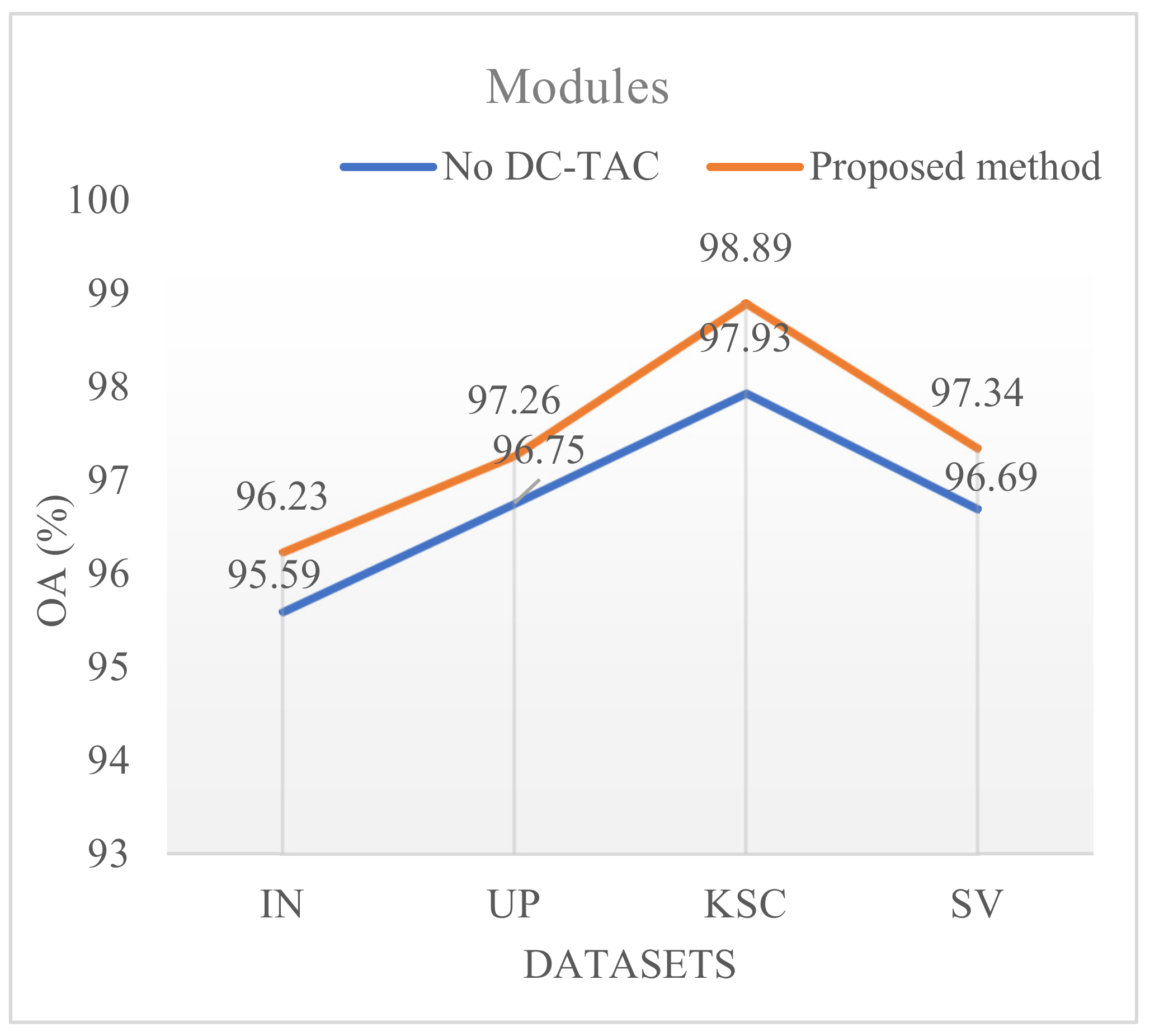
(3) DC-TAC: Using OA as a measure of classification performance, we performed some comparative experiments to verify the classification performance of the proposed DC-TAC module. The designed comparison experiment was as follows: using 3D-CNNs instead of DC-TAC of the proposed method, recorded as “no DC-TAC,” we performed experiments on four datasets: IN, UP, KSC, and SV. Figure 13 shows the classification results of the experiment. By looking at the classification results in Figure 13, we can see that the OA obtained by the proposed method was the highest. The OA without DC-TAC on the IN dataset was 0.64% lower than that obtained by the proposed method; the OA of the proposed method on the UP dataset was 0.51% higher than that without DC-TAC; the OA without DC-TAC on the KSC dataset was 0.96% lower than that obtained by the proposed method; and the OA of the proposed method on the SV dataset was 0.65% higher than that without DC-TAC. By observing the above experimental results, it can be found that the proposed DC-TAC module was beneficial in improving classification performance.

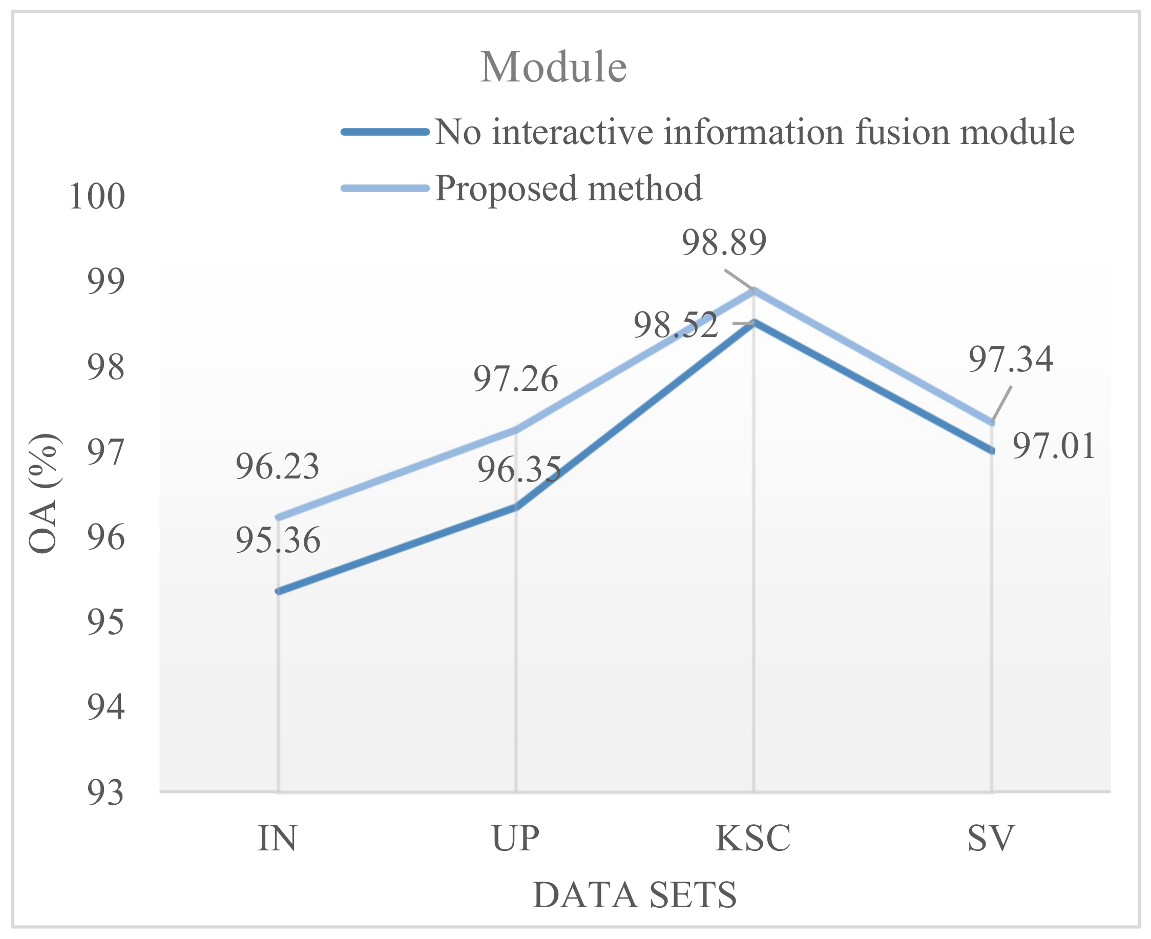
(4) Interactive information fusion module: The proposed information fusion module can integrate the rich spectral information contained in the spatial features extracted from the spatial branches into the spectral features extracted from the spectral branches. Similarly, the spectral features extracted by the same spectral branches contain rich spatial information and can be fused with spatial features. In order to better verify the performance of the proposed information fusion module, the classification results of the module with and without the information fusion module were compared. The experimental results of the two experiments are shown in Figure 14. It can be easily found from Figure 14 that the classification performance of the proposed method was better than that of the method without the information fusion module. The experimental results proved that the information fusion module was helpful in improving the classification performance of hyperspectral images.

4.2. The Influence of the Proportion of Training Samples on the Experimental Results

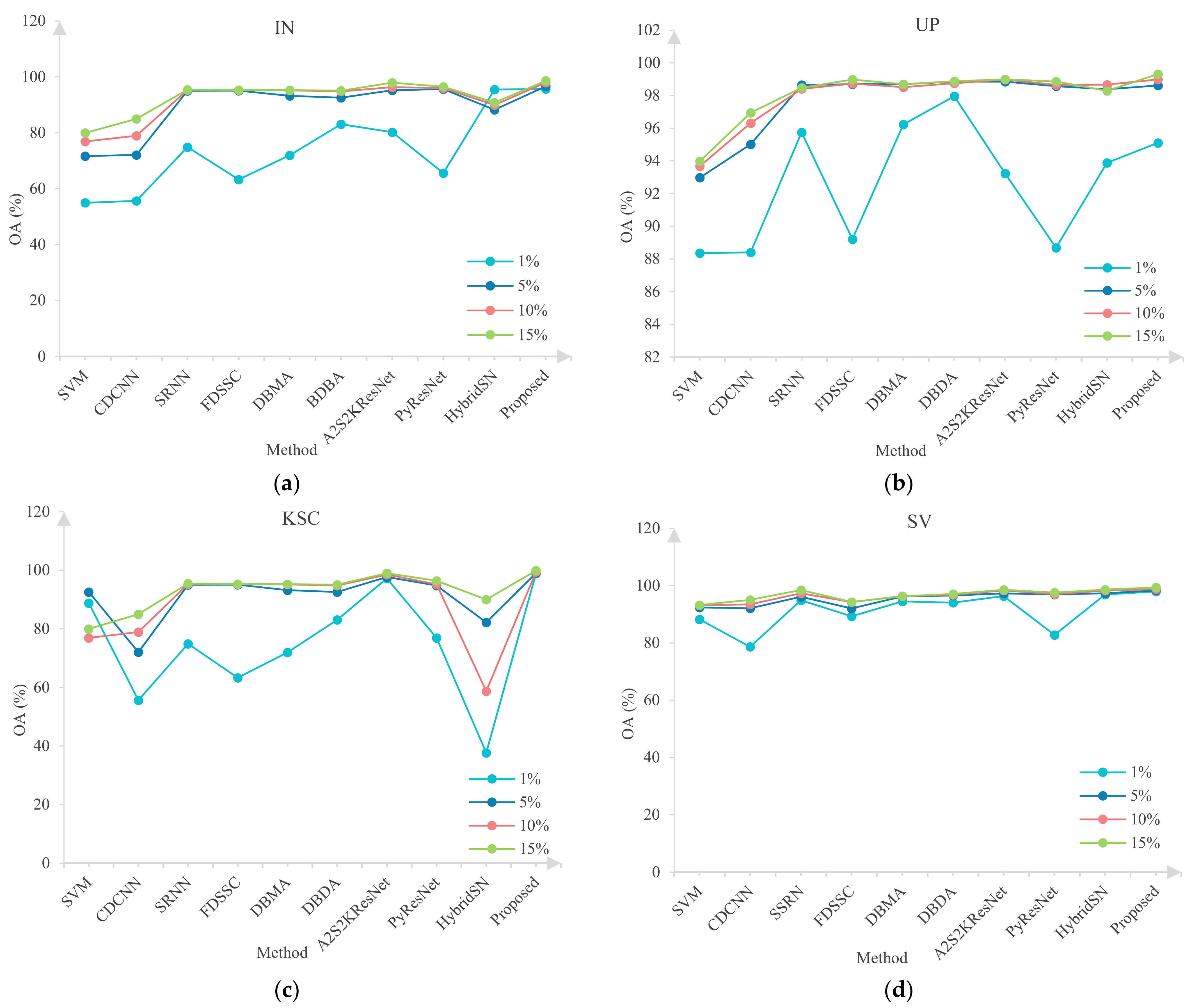
In this experiment, four datasets were used, i.e., IN, UP, KSC, and SV, to carry out validation experiments with training samples of different sizes. The performance of the proposed module and the comparison module was verified. From the datasets, 5%, 10%, and 15% were randomly selected as training samples to train the proposed module and other comparison modules. Figure 15 shows the classification results of each method on the four well-known geographic datasets: IN, UP, KSC, and SV.

From the observation in Figure 15, it can be seen that when a small number of training samples were used, the proposed method was the best, while the performances of CDCNN and SVM were relatively poor. The classification accuracy of each method increased with the number of training samples from the four datasets (IN, UP, KSC, and SV), but the proposed method still achieved higher classification accuracy. The experimental results showed that this method had a good ability to increase the feature effectiveness of the high-dimensional spectral images.

5. Conclusions

In this paper, a new end-to-end network for hyperspectral image classification is proposed. Firstly, a 3D-OCONV is designed and introduced into the spatial branch and spectral branch, respectively. This module can make the fusion of high-frequency and low-frequency information better integrated; at the same time, the network parameters can be reduced. Subsequently, the mechanism of spectral attention in spectral branching and 3D-MSSAM in spatial branching were developed to highlight important spatial regions and spectral bands to enhance the ability of feature representation. To further extract spectral and spatial information at different scales, a DC-TAC is proposed to further capture the useful information of the two branches. At the end, an interactive information fusion module was designed, which allowed the spatial and spectral information acquired by the two branches to be brought together interactively. The final result of the experiment showed that even if there were few training samples, this method could still achieve good classification performance. In the future, we will do some work to make the network simpler and have fewer network parameters, which will shorten the training time and further improve the classification performance of hyperspectral images.

References

1. Wei, X.; Li, W.; Zhang, M.; Li, Q. Medical Hyperspectral Image Classification Based on End-to-End Fusion Deep Neural Network. IEEE Trans. Instrum. Meas. 2019, 68, 4481–4492. [Google Scholar] [CrossRef]
2. Patel, N.K.; Patnaik, C.; Dutta, S.; Shekh, A.M.; Dave, A.J. Study of crop growth parameters using airborne imaging spectrometer data. Int. J. Remote Sens. 2001, 22, 2401–2411. [Google Scholar] [CrossRef]
3. Feng, L.; Zhu, S.; Zhou, L.; Zhao, Y.; Bao, Y.; Zhang, C.; He, Y. Detection of Subtle Bruises on Winter Jujube Using Hyperspectral Imaging with Pixel-Wise Deep Learning Method. IEEE Access 2019, 7, 64494–64505. [Google Scholar] [CrossRef]
4. Xu, Y.; Du, B.; Zhang, F.; Zhang, L. Hyperspectral image classification via a random patches network. ISPRS J. Photogramm. Remote Sens. 2018, 142, 344–357. [Google Scholar] [CrossRef]
5. Zhang, X.; Sun, Y.; Jiang, K.; Li, C.; Jiao, L.; Zhou, H. Spatial Sequential Recurrent Neural Network for Hyperspectral Image Classification. IEEE J. Sel. Top. Appl. Earth Obs. Remote Sens. 2018, 11, 4141–4155. [Google Scholar] [CrossRef] [Green Version]
6. Heylen, R.; Parente, M.; Gader, P. A Review of Nonlinear Hyperspectral Unmixing Methods. IEEE J. Sel. Top. Appl. Earth Obs. Remote Sens. 2014, 7, 1844–1868. [Google Scholar] [CrossRef]
7. Li, W.; Du, Q. Collaborative Representation for Hyperspectral Anomaly Detection. IEEE Trans. Geosci. Remote Sens. 2015, 53, 1463–1474. [Google Scholar] [CrossRef]
8. Ma, X.; Zhang, X.; Tang, X.; Zhou, H.; Jiao, L. Hyperspectral Anomaly Detection Based on Low-Rank Representation with Data-Driven Projection and Dictionary Construction. IEEE J. Sel. Top. Appl. Earth Obs. Remote Sens. 2020, 13, 2226–2239. [Google Scholar] [CrossRef]
9. Delalieux, S.; Somers, B.; Haest, B.; Spanhove, T.; Vanden Borre, J.; Mücher, C.A. Heathland conservation status mapping through integration of hyperspectral mixture analysis and decision tree classififiers. Remote Sens. Environ. 2012, 126, 222–231. [Google Scholar] [CrossRef]
10. Ham, J.; Chen, Y.; Crawford, M.M.; Ghosh, J. Investigation of the random forest framework for classification of hyperspectral data. IEEE Trans. Geosci. Remote Sens. 2005, 43, 492–501. [Google Scholar] [CrossRef]
11. Gualtieri, J.A.; Chettri, S. Support vector machines for classification of hyperspectral data. In Proceedings of the International Geoscience and Remote Sensing Symposium (IGARSS), Honolulu, HI, USA, 24–28 July 2000; Volume 2, pp. 813–815. [Google Scholar]
12. Li, W.; Du, Q. A survey on representation-based classification and detection in hyperspectral remote sensing imagery. Pattern Recognit. Lett. 2016, 83, 115–123. [Google Scholar] [CrossRef]
13. Soltani-Farani, A.; Rabiee, H.R.; Hosseini, S.A. Spatial-Aware Dictionary Learning for Hyperspectral Image Classification. IEEE Trans. Geosci. Remote Sens. 2015, 53, 527–541. [Google Scholar] [CrossRef] [Green Version]
14. Zhao, J.; Zhong, Y.; Jia, T.; Wang, X.; Xu, Y.; Shu, H.; Zhang, L. Spectral-spatial classification of hyperspectral imagery with cooperative game. ISPRS J. Photogramm. Remote Sens. 2018, 135, 31–42. [Google Scholar] [CrossRef]
15. Li, J.; Bioucas-Dias, J.M.; Plaza, A. Spectral-spatial hyperspectral image segmentation using subspace multinomial logistic regression and Markov random fifields. IEEE Trans. Geosci. Remote Sens. 2012, 50, 809–823. [Google Scholar] [CrossRef]
16. Cao, X.; Wang, X.; Wang, D.; Zhao, J.; Jiao, L. Spectral–Spatial Hyperspectral Image Classification Using Cascaded Markov Random Fields. IEEE J. Sel. Top. Appl. Earth Obs. Remote Sens. 2019, 12, 4861–4872. [Google Scholar] [CrossRef]
17. Li, G.; Li, L.; Zhu, H.; Liu, X.; Jiao, L. Adaptive Multiscale Deep Fusion Residual Network for Remote Sensing Image Classification. IEEE Trans. Geosci. Remote Sens. 2019, 57, 8506–8521. [Google Scholar] [CrossRef]
18. Ronneberger, O.; Fischer, P.; Brox, T. U-Net: Convolutional Networks for Biomedical Image Segmentation. In Proceedings of the International Conference on Medical Image Computing and Computer-Assisted Intervention, arXiv, Computer Science, Computer Vision and Pattern Recognition, Munich, Germany, 18 May 2015; Volume 9351, pp. 234–241. [Google Scholar]
19. Wang, R.J.; Li, X.; Ling, C.X. Pelee: A Real-Time Object Detection System on Mobile Devices. In Computer Vision and Pattern Recognition; Cornell University: Ithaca, NY, USA, 2018; Volume 10, p. 1804.06882. [Google Scholar]
20. Zeng, D.; Liu, K.; Chen, Y.; Zhao, J. Distant Supervision for Relation Extraction via Piecewise Convolutional Neural Networks. In Proceedings of the 2015 Conference on Empirical Methods in Natural Language Processing, Lisbon, Portugal, 17–21 September 2015; Volume 9. [Google Scholar]
21. Gehring, J.; Auli, M.; Grangier, D.; Yarats, D.; Dauphin, Y.N. Convolutional Sequence to Sequence Learning. In Proceedings of the Machine Learning Research, Sydney, Australia, 6–11 August 2017; Volume 70, pp. 1243–1252. [Google Scholar]
22. He, H.; Gimpel, K.; Lin, J. Multi-Perspective Sentence Similarity moduleing with Convolutional Neural Networks. Nat. Lang. Process. 2015, 26–31, 1576–1586. [Google Scholar]
23. Alipourfard, T.; Arefi, H.; Mahmoudi, S. A Novel Deep Learning Framework by Combination of Subspace-based Feature Estraction and Convolutional Neural Networks for Hyperspectral Images Classification. In Proceedings of the IEEE IGARSS, Valencia, Spain, 22–27 July 2018; Volume 13. [Google Scholar]
24. Huang, K.-K.; Ren, C.-X.; Liu, H.; Lai, Z.-R.; Yu, Y.-F.; Dai, D.-Q. Hyperspectral Image Classification via Discriminant Gabor Ensemble Filter. IEEE Trans. Cybern. 2021, 52, 8352–8365. [Google Scholar] [CrossRef]
25. Ding, Y.; Zhao, X.; Zhang, Z.; Cai, W.; Yang, N.; Zhan, Y. Semi-Supervised Locality Preserving Dense Graph Neural Network with ARMA Filters and Context-Aware Learning for Hyperspectral Image Classification. IEEE Trans. Geosci. Remote Sens. 2021, 60, 1–12. [Google Scholar] [CrossRef]
26. Kang, X.; Li, C.; Li, S.; Lin, H. Classification of Hyperspectral Images by Gabor Filtering Based Deep Network. IEEE J. Sel. Top. Appl. Earth Obs. Remote Sens. 2018, 11, 1166–1178. [Google Scholar] [CrossRef]
27. Filipović, V.; Panić, M.; Bhardwaj, K. Morphological Complexity Profile for the Analysis of Hyperspectral Images; IEEE: Piscataway, NJ, USA, 2021; Volume 12, pp. 1–6. [Google Scholar]
28. Zhang, X.; Gao, Z.; Jiao, L.; Zhou, H. Multifeature Hyperspectral Image Classification with Local and Nonlocal Spatial Information via Markov Random Field in Semantic Space. IEEE Trans. Geosci. Remote Sens. 2018, 56, 1409–1424. [Google Scholar] [CrossRef]
29. Tu, B.; Huang, S.; Fang, L.; Zhang, G.; Wang, J.; Zheng, B. Hyperspectral Image Classification via Weighted Joint Nearest Neighbor and Sparse Representation. IEEE J. Sel. Top. Appl. Earth Obs. Remote Sens. 2018, 11, 4063–4075. [Google Scholar] [CrossRef]
30. Ehsan, U.A.M. Feature Subspace Detection for Hyperspectral Images Classification using Segmented Principal Component Analysis and F-score. In Proceedings of the 2020 IEEE Region 10 Symposium (TENSYMP), Dhaka, Bangladesh, 5–7 June 2020; IEEE: Piscataway, NJ, USA, 2020; pp. 134–137. [Google Scholar]
31. Wang, J.; Zhong, Y.; Zheng, Z.; Ma, A.; Zhang, L. RSNet: The Search for Remote Sensing Deep Neural Networks in Recognition Tasks. IEEE Trans. Geosci. Remote Sens. 2021, 59, 2520–2534. [Google Scholar] [CrossRef]
32. Liu, C.; Ma, J.; Tang, X.; Liu, F.; Zhang, X.; Jiao, L. Deep Hash Learning for Remote Sensing Image Retrieval. IEEE Trans. Geosci. Remote Sens. 2021, 59, 3420–3443. [Google Scholar] [CrossRef]
33. Chen, Y.; Zhao, X.; Jia, X. Spectral-Spatial classification of hyperspectral data based on deep belief network. IEEE J. Sel. Topics Appl. Earth Observ. Remote Sens. 2015, 8, 2381–2392. [Google Scholar] [CrossRef]
34. Tao, C.; Pan, H.; Li, Y.; Zou, Z. Unsupervised Spectral–Spatial Feature Learning with Stacked Sparse Autoencoder for Hyperspectral Imagery Classification. IEEE Geosci. Remote Sens. Lett. 2015, 12, 2438–2442. [Google Scholar]
35. He, K.; Zhang, X.; Ren, S.; Sun, J. Deep residual learning for image recognition. In Proceedings of the IEEE Conference on Computer Vision and Pattern Recognition (CVPR), Las Vegas, NV, USA, 27–30 June 2016; pp. 770–778. [Google Scholar]
36. Sabour, S.; Frosst, N.; Hinton, G.E. Dynamic routing between capsules. In Proceedings of the Advances in Neural Information Processing Systems, Long Beach, CA, USA, 4–9 December 2017; pp. 3856–3866. [Google Scholar]
37. Huang, G.; Liu, Z.; Van Der Maaten, L.; Weinberger, K.Q. Densely connected convolutional networks. In Proceedings of the IEEE Conference on Computer Vision and Pattern Recognition (CVPR), Honolulu, HI, USA, 21–26 July 2017; pp. 4700–4708. [Google Scholar]
38. Han, K.; Wang, Y.; Tian, Q.; Guo, J.; Xu, C.; Xu, C. Noah’s Ark Lab. Huawei Technologies. In GhostNet: More Features from Cheap Operations; No. 00165; IEEE: Piscataway, NJ, USA, 2020. [Google Scholar]
39. Chen, Y.; Li, J.; Xiao, H.; Jin, X.; Yan, S.; Feng, J. Dual path networks. In Proceedings of the Advances in Neural Information Processing Systems, Long Beach, CA, USA, 4–9 December 2017; Volume 9, pp. 4467–4475. [Google Scholar]
40. Paoletti, M.E.; Haut, J.M.; Fernandez-Beltran, R.; Plaza, J.; Plaza, A.J.; Pla, F. Deep Pyramidal Residual Networks for Spectral–Spatial Hyperspectral Image Classification. IEEE Trans. Geosci. Remote Sens. 2019, 57, 740–754. [Google Scholar] [CrossRef]
41. Paoletti, M.E.; Haut, J.M.; Plaza, J.; Plaza, A. Deep&Dense Convolutional Neural Network for Hyperspectral Image Classification. Remote Sens. 2018, 10, 1454. [Google Scholar]
42. Paoletti, M.E.; Haut, J.M.; Fernandez-Beltran, R.; Plaza, J.; Plaza, A.; Li, J.; Pla, F. Capsule networks for hyperspectral image classification. IEEE Trans. Geosci. Remote Sens. 2019, 57, 2145–2160. [Google Scholar] [CrossRef]
43. Kang, X.; Zhuo, B.; Duan, P. Dual-Path Network-Based Hyperspectral Image Classification. IEEE Geosci. Remote Sens. Lett. 2019, 16, 447–451. [Google Scholar] [CrossRef]
44. Shuai, B.; Zuo, Z.; Wang, B.; Wang, G. DAG-recurrent neural networks for scene labeling. In Proceedings of the IEEE Conference on Computer Vision and Pattern Recognition (CVPR), Las Vegas, NV, USA, 27–30 June 2016; pp. 3620–3629. [Google Scholar]
45. Chen, Y.; Lin, Z.; Zhao, X.; Wang, G.; Gu, Y. Deep Learning-Based Classification of Hyperspectral Data. IEEE J. Sel. Top. Appl. Earth Obs. Remote Sens. 2014, 7, 2094–2107. [Google Scholar] [CrossRef]
46. Liu, Q.; Dong, Y.; Zhang, Y.; Luo, H. A Fast Dynamic Graph Convolutional Network and CNN Parallel Network for Hyperspectral Image Classification. IEEE Trans. Geosci. Remote Sens. 2022, 60, 5530215. [Google Scholar] [CrossRef]
47. Zhang, X.; Chen, S.; Zhu, P.; Tang, X.; Feng, J.; Jiao, L. Spatial Pooling Graph Convolutional Network for Hyperspectral Image Classification. IEEE Trans. Geosci. Remote Sens. 2022, 60, 5521315. [Google Scholar] [CrossRef]
48. Haut, J.M.; Paoletti, M.E.; Plaza, J.; Plaza, A.; Li, J. Visual attention-driven hyperspectral image classifification. IEEE Trans. Geosci. Remote Sens. 2019, 57, 8065–8080. [Google Scholar] [CrossRef]
49. Li, R.; Zheng, S.; Duan, C.; Yang, Y.; Wang, X. Classification of Hyperspectral Image Based on Double-Branch Dual-Attention Mechanism Network. Remote Sens. 2020, 12, 582. [Google Scholar] [CrossRef] [Green Version]
50. Chen, Y.; Jiang, H.; Li, C.; Jia, X.; Ghamisi, P. Deep feature extraction and classifification of hyperspectral images based on convolutional neural networks. IEEE Trans. Geosci. Remote Sens. 2016, 54, 6232–6251. [Google Scholar] [CrossRef] [Green Version]
51. Zhong, Z.; Li, J.; Luo, Z.; Chapman, M. Spectral–Spatial Residual Network for Hyperspectral Image Classification: A 3-D Deep Learning Framework. IEEE Trans. Geosci. Remote Sens. 2017, 56, 847–858. [Google Scholar] [CrossRef]
52. Wang, W.; Dou, S.; Jiang, Z.; Sun, L. A Fast Dense Spectral–Spatial Convolution Network Framework for Hyperspectral Images Classification. Remote Sens. 2018, 10, 1068. [Google Scholar] [CrossRef] [Green Version]
53. Ma, W.; Yang, Q.; Wu, Y.; Zhao, W.; Zhang, X. Double-Branch Multi-Attention Mechanism Network for Hyperspectral Image Classification. Remote Sens. 2019, 11, 1307. [Google Scholar] [CrossRef] [Green Version]
54. Feng, J.; Wu, X.; Shang, R.; Sui, C.; Li, J.; Jiao, L.; Zhang, X. Attention Multibranch Convolutional Neural Network for Hyperspectral Image Classification Based on Adaptive Region Search. IEEE Trans. Geosci. Remote Sens. 2021, 59, 5054–5070. [Google Scholar] [CrossRef]
55. Yang, B.; Hu, S.; Guo, Q.; Hong, D. Multisource Domain Transfer Learning Based on Spectral Projections for Hyperspectral Image Classification. IEEE J. Sel. Top. Appl. Earth Obs. Remote Sens. 2022, 15, 3730–3739. [Google Scholar] [CrossRef]
56. Yu, C.; Han, R.; Song, M. Feedback Attention-Based Dense CNN for Hyperspectral Image Classification. IEEE Trans. Geosci. Remote Sens. 2021, 60, 5501916. [Google Scholar] [CrossRef]
57. Dundar, T.; Ince, T. Sparse Representation-Based Hyperspectral Image Classification Using Multiscale Superpixels and Guided Filter. IEEE Trans. Geosci. Remote Sens. 2019, 16, 246–250. [Google Scholar] [CrossRef]
58. Chen, Y.; Fan, H.; Xu, B.; Yan, Z.; Kalantidis, Y.; Rohrbach, M.; Yan, S.; Feng, J. Drop an Octave: Reducing Spatial Redundancy in Convolutional Neural Networks with Octave Convolution. In Proceedings of the Computer Vision and Pattern Recognition, Long Beach, CA, USA, 16–20 June 2019; pp. 3435–3444. [Google Scholar]
59. Dai, Y.; Gieseke, F.; Oehmcke, S.; Wu, Y.; Barnard, K. Attentional Feature Fusion. In Proceedings of the IEEE/CVF Winter Conference on Applications of Computer Vision (WACV), Online, 5–9 January 2021; pp. 3560–3569. [Google Scholar]
60. Roy, S.K.; Manna, S.; Song, T.; Bruzzone, L. Attention-Based Adaptive Spectral–Spatial Kernel ResNet for Hyperspectral Image Classification. IEEE Trans. Geosci. Remote Sens. 2020, 59, 7831–7843. [Google Scholar] [CrossRef]
61. Lee, H.; Kwon, H. Going Deeper with Contextual CNN for Hyperspectral Image Classification. IEEE Trans. Image Process. 2017, 26, 4843–4855. [Google Scholar] [CrossRef] [Green Version]
62. Roy, S.K.; Krishna, G.; Dubey, S.R.; Chaudhuri, B.B. HybridSN: Exploring 3-D–2-D CNN Feature Hierarchy for Hyperspectral Image Classification. IEEE Geosci. Remote Sens. Lett. 2020, 17, 277–281. [Google Scholar] [CrossRef] [Green Version]
63. Melgani, F.; Bruzzone, L. Classification of hyperspectral remote sensing images with support vector machines. IEEE Trans. Geosci. Remote Sens. 2004, 42, 1778–1790. [Google Scholar] [CrossRef]
64. Heo, B.; Yun, S.; Han, D.; Chun, S.; Choe, J.; Oh, S.J. Rethinking Spatial Dimensions of Vision Transformers. In Proceedings of the 2021 IEEE/CVF International Conference on Computer Vision (ICCV), Montreal, QC, Canada, 11–17 October 2021; pp. 11916–11925. [Google Scholar]
Figure 1. Overall schematic diagram of the proposed method.
Remotesensing 15 00257 g001
Figure 2. Schematic diagram of the three-dimensional octave convolution.
Remotesensing 15 00257 g002
Figure 3. Schematic diagram of octave convolution.
Remotesensing 15 00257 g003
Figure 4. Schematic diagram of 3D-MSSAM.
Remotesensing 15 00257 g004
Figure 5. The schematic diagram of spectral attention module.
Remotesensing 15 00257 g005
Figure 6. Schematic diagram of multiscale asymmetric convolution.
Remotesensing 15 00257 g006
Figure 7. Schematic diagram of the information fusion module.
Remotesensing 15 00257 g007
Figure 8. The overall accuracy and classification maps of different methods on IN dataset: (a) A2S2KResNe (92.1%); (b) DBDA (92.58%); (c) DBMA (89.95%); (d) PyResNet (51.03%); (e) SSRN (89.24%); (f) ViT (78.62%); (g) SVM (67.77%); (h) HybridSN (82.18%); (i) DCCNN (71.42%); (j) FDSSC (92.29%); (k) proposed (96.23%).
Remotesensing 15 00257 g008
Figure 9. The overall accuracy and classification maps of different methods on UP dataset: (a) A2S2KResNe (87.44%); (b) DBDA (96.01%); (c) DBMA (91.8%); (d) PyResNet (54.64%); (e) SSRN (92.50%); (f) ViT (93.23%); (g) SVM (83.03%); (h) HybridSN (81.85%); (i) DCCNN (87.94%); (j) FDSSC (93.16%); (k) proposed (97.26%).
Remotesensing 15 00257 g009
Figure 10. The overall accuracy and classification maps of different methods on SV dataset: (a) A2S2KResNe (94.58%); (b) DBDA (93.74%); (c) DBMA; (d) PyResNet (91.51%); (e) SSRN (92.04%); (f) ViT (95.79%); (g) SVM (86.98%); (h) HybridSN (87.33%); (i) CDCNN (88.36%); (j) FDSSC (95.79%); (k) proposed (97.34%).
Remotesensing 15 00257 g010
Figure 11. The overall accuracy and classification maps of different methods on the KSC dataset: (a) A2S2KResNe (91.22%); (b) DBDA (96.76%); (c) DBMA (94.12%); (d) PyResNet (91.49%); (e) SSRN (95.52%); (f) ViT (92.38%); (g) SVM (87.96%); (h) HybridSN (79.72%); (i) DCCNN (89.33%); (j) FDSSC (95.62%); (k) proposed (98.89%).
Remotesensing 15 00257 g011
Figure 12. OAs of 3D-CNNs and 3D-OCONV on IN, UP, KSC, and SV datasets (%).
Remotesensing 15 00257 g012
Figure 13. OAs with different feature extraction modules on IN, UP, KSC, and SV datasets (%).
Remotesensing 15 00257 g013
Figure 14. OAs with different feature extraction modules on IN, UP, KSC, and SV datasets (%).
Remotesensing 15 00257 g014
Figure 15. Classification performance of different methods under different training sample ratios on IN, UP, SV, and KSC datasets: (a) classification results on IN dataset; (b) classification results on the UP dataset; (c) classification results on the SV dataset; (d) classification results on the KSC dataset.
Remotesensing 15 00257 g015