1. Introduction
Soil erosion is becoming a major land deterioration hazard worldwide. Making strides in our understanding of the likely future rates of soil erosion, quickened by human activity and climate alterations, is one of the foremost conclusive components when it comes to making choices on preservation arrangements and for Earth ecosystem modelers looking to diminish the unreliability of global expectations [
1]. Despite this, detailed information is typically based on limited field campaigns and is typically only known locally [
2].
This is the situation in Iceland, where Landgræðslan, the country’s Soil Conservation Service, is the sole source of the majority of information about soil degradation in the land [
3]. The deterioration of Iceland’s ecosystem can be considered as a form of desertification. Due to their lack of vegetation, its badlands have prominent similitudes to desolate zones in dry weathered nations. Soil erosion forecast plays a key part in relieving such progression [
4].
From a historical perspective, pioneers include Björn Johannesson [
5], who first published a soil erosion map in his book on the soils of Iceland. The current FAO classification for Icelandic soils was attempted decades later [
6]. The Agricultural Research Institute of Iceland (Rala), which became a part of the Agricultural University of Iceland (AUI) in 2005, has done the majority of the work on Icelandic soil science. The joint European COST-622 Action [
7,
8] provides a wealth of information regarding the chemical and physical properties of Iceland’s soils. Numerous Icelandic and international research efforts have contributed to our understanding of the effects of both man-caused and natural degradation.
The government of Iceland aspires to control soil erosion and achieve sustainable land use as soon as possible. The interaction of past and present grazing effects with delicate soils and vegetation is the primary cause of desertification. In order to better manage and monitor grazing practices in protected areas that are at risk of erosion and to restore denuded land, the soil conservation authorities—primarily the soil conservation service—were given stronger capabilities [
9].
Measurements taken on the ground and aerial photographs taken at various points in time are two of the methods used to evaluate the progression of soil erosion. With aerial photographs, there are two methods: scanning and image analysis on one hand, and digitizing on the other. There is a certain amount of room for error when using them, however. On-site measurement is difficult because these are expensive tasks, especially in some parts of the country where access is difficult. As a result, not all areas of interest can currently be investigated.
Soil erosion in Arctic regions such as Iceland may also have an impact on the global climate, in addition to the effects that climate change may already be having on the ecosystems of those regions. Up to half of the carbon in the soil of Earth is stored in northern latitudes; approximately twice as much carbon as is stored in the atmosphere. The significance of this carbon sink cannot be overstated. Northern circumpolar soils are a significant carbon sink because of extensive peatlands and permanently frozen ground that keeps this organic carbon locked up in the soil [
10]. The Northern Circumpolar Soil Carbon Database’s most recent estimates indicate that the northern permafrost region contains approximately 1672 Pg of organic carbon, with approximately 1466 Pg, or 88%, occurring in soils and deposits that are perpetually frozen [
11]. Thermal collapse and erosion of these carbon-rich deposits may accelerate with Arctic amplification of climate warming [
12].
Through the development of satellite remote sensing technology, one extremely useful tool has been made available to overcome the limitations outlined above [
13]. Its application to evaluate soil erosion, in any event, when in view of uninhibitedly available satellite information, has resulted in numerous breakthroughs as of late [
14,
15]. Some multi-resolution approaches to soil erosion risk mapping have been used in previous studies, but they only used indicators such as rainfall and vegetation cover to apply them to Iceland.
In this work, ground truth samples are used in our proposed solution to analyse pre-processed remote images over a specific area, to then automate the analysis for larger, more difficult-to-access areas. This solution is being developed specifically for Icelandic soil erosion studies, using Sentinel-2 satellite data combined with Landgræðslan’s local assessment data. Given that they are the oldest soil erosion department in the world, their historical data is more extensive than usual.
This is made possible by training a machine learning (ML) algorithm that can produce appropriate weights that represent erosion-prone areas using a set of geo-environmental parameters. In operation research, the development of mathematical and computational tools to support decision makers’ intellectual evaluation of criteria and alternatives has been incorporating an increasing number of ML models [
16]. Training the algorithm requires parameters of bare ground cover, which can be calculated solely from satellite images by using information from observationally correct areas devoid of vegetation as a calibration; Icelandic soil profiles, which will be examined to determine how the profile relates to the intensity of soil erosion; as well as data on arable land, including cultivated land plant species, and the parameters of agriculture use. These are all included in the available data.
One of the areas of ML where inputs can be given a class label is classification. Image classification has been the focus of several remote sensing applications using Random Forest (RF), Support Vector Machine (SVM), and Multilayer Perceptron (MLP) among the available ML algorithms. One of the hot topics in multiple research fields that use images of different resolutions taken by different platforms, while including several limitations and priorities, is how to choose the best image classification algorithm.
Based on the authors’ knowledge, there are very few studies that have focused on applying these methods to the study of soil erosion in Arctic areas, despite machine learning models potentially being very competitive in terms of accuracy and predictive power. Similar image processing classification techniques have been used to study the arctic tundra vegetation [
17], the ionic composition of arctic lakes [
18] and land cover types [
19]. Deep learning has been employed to monitor polar sea ice [
20].
Regarding soil erosion, early remote sensing studies showed an increase in erosion rate during the last decades in areas such as Alaska [
21]. Contemporary techniques are throwing interesting conclusions that link coastal erosion to sea surface temperature fluctuations [
22] and complex processes related to coastal permafrost bluff erosion [
23]. In fact, deep learning techniques were recently applied to extract the erosion rates of Arctic permafrost [
24]. As such, this is an exciting area in which many discoveries are yet to be made. Particularly, there is a lack of detailed analyses of the influence of slope steepness and height on erosion, since these are factors that do not play an important role in other areas of the world. The present study aims at providing one of the first steps toward establishing the most reliable, fast and accurate classical ML algorithm to predict soil erosion quantitatively in the Arctic, which may in turn allow us to locate the main process driving it.
2. Materials and Methods
2.1. Data and Preprocessing
2.1.1. Icelandic Soil Erosion Data
Iceland is an island of size 103,000 km
2 located within the Arctic Circle that presents a unique combination of erosion factors not seen in any other region on the planet. The region experiences high levels of volcanic and seismic activity due to its position over a hotspot on the Mid-Atlantic Ridge (a divergent tectonic plate boundary), as well as a harsh climate of cold winters and cool summers due to the moderating effects of the Atlantic Gulf Stream [
25,
26]. Its unique geography and weather include glaciers (which cover 11% of its surface and are melting), very active volcanoes, carbon rich volcanic soils, sand dunes, freeze-thaw cycles and extreme winds. The landscape is sparsely vegetated (<50% of land is vegetation) and there is little to no tree cover, which is a relatively recent change that resulted from livestock overgrazing and human activity paired with the harsh climates, winds and volcanic activity [
27,
28], the effects of which are still felt today. Vegetation loss exposes top layers of soil, which are easily disturbed by wind erosion [
29,
30]. Moreover, volcanic eruptions can produce large dust storms that further threaten vegetation, and melting glaciers from volcanic activity can impact soil through water erosion [
26,
27,
29].
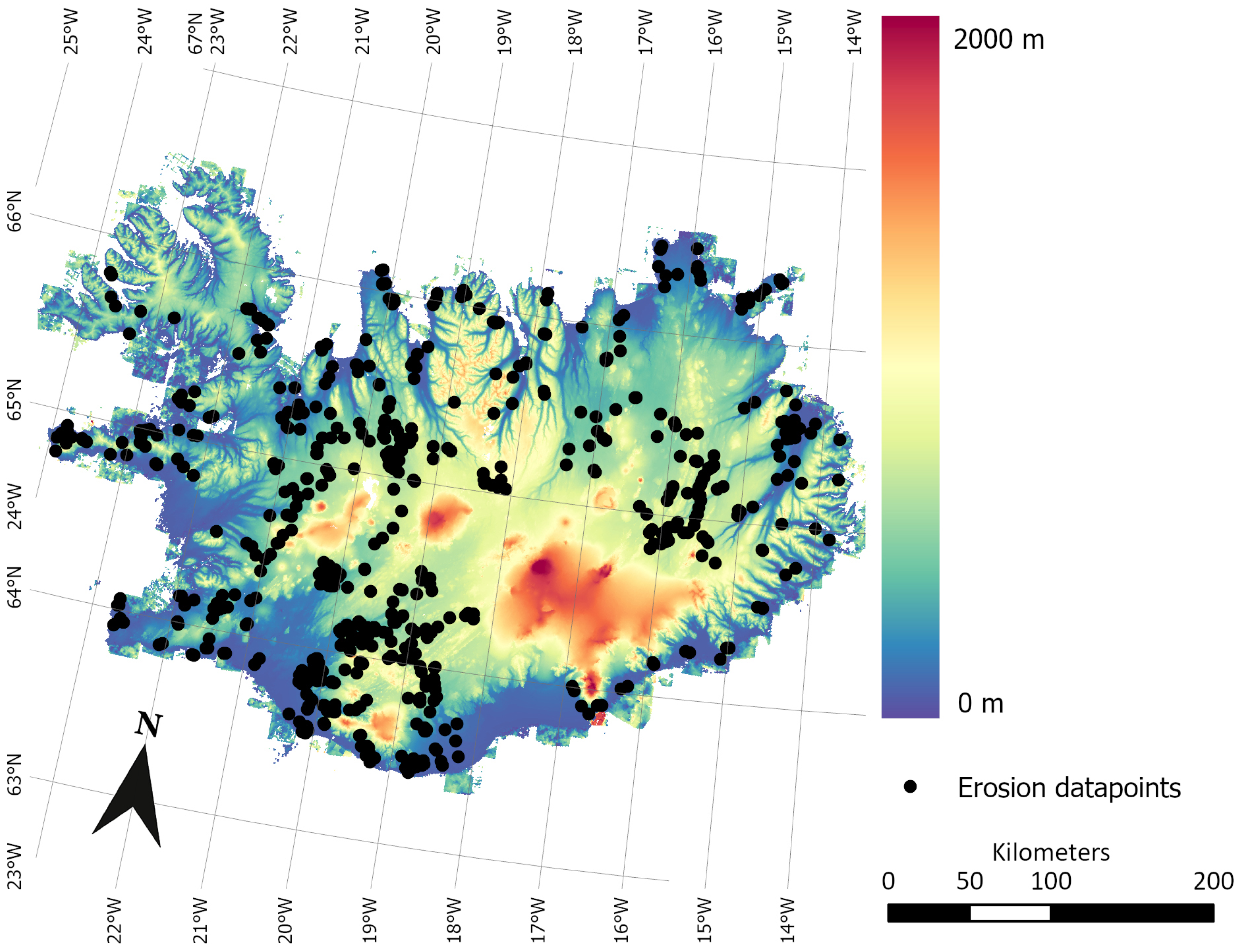
With the continued threat of erosion and degradation, the Soil Conservation Service of Iceland, known as Landgræðslan, monitors and assesses the level of soil erosion across Iceland as part of its efforts to protect, restore and improve the island’s vegetation and soil resources. Some of this data on soil erosion levels was provided to us by the organisation, consisting of a database of 748 regions, which are visualised in
Figure 1. Each point consists of a value reflecting the measured level of soil erosion within the region, which was used as ground truth values for our training data. This data was obtained through various programmes of assessment aimed at land restoration, since the scale of soil erosion and desertification in Iceland has long been a cause of ecological concern in the country [
29].
2.1.2. Earth Observations Data
The Copernicus Sentinel-2 data, characterized by its free access policy, has a global coverage of Earth’s land surfaces from 56° S to 84° N. It offers improved data compared to other low spatial resolution satellite images, especially in temporal and spatial resolution [
31]. The 13 bands for Sentinel-2 images have spatial resolutions ranging from 10 to 60 m [
32]. The other valuable characteristic of Sentinel-2 data is its high temporal resolution of 5 days [
33]. Its sensor has low radiometric calibration uncertainty that makes the radiance of the images to produce reliable results. Thus, Sentinel-2 images have the potential to produce highly accurate information and to support different applications [
13].
The data we used to train our machine learning models was obtained through WEkEO, the European Union Copernicus DIAS reference service, which provides pre-processed L2A Sentinel-2 data. The data consists of geo-referenced and atmospherically corrected images of Iceland between 23 June 2015 and 26 July 2022. Scene classification layers are included for each picture, which can be projected into the original in order to figure out which pixels depict snow, clouds or non-information areas. After that, an automated procedure is used to create a combined image without these undesirable effects. This was performed with images taken over a 30-day summer period for the present results. Depending on the satellite pass, the data are accessible every 5 to 10 days [
34].
We generated images of all over Iceland for each band between 2 July 2019 and 24 September 2021. We decided to focus on bands with resolutions between 10 and 20 m. After atmospheric correction, pixels either with clouds or shadows of clouds, or with no data or overly saturated (surface reflectance greater than 1) were considered as bad pixels. The latter may happen due to sub glint or snow reflectance. Snow and ice should also be removed, as well as water bodies, which are of no interest if they are constantly full. After cropping clouds and bad pixels out, these images are then used to create indices [
35]. Indices that represent or highlight particular characteristics, such as vegetation, soil crusting, bare soil, and red edge indices, were created by combining data from various spectral bands.
The raw Sentinel-2 images may appear changed between different dates and thus require appropriate data filtering. This is a challenging task, since our atmosphere is quite dynamic and can change for many reasons. Even after cloudy observations have been filtered out by the preprocessing system [
36] of Sentinel-2, some cloud shadows are misclassified by default and therefore artifacts are still present. What is left is a mixture of valid observations and a set of undetected anomalous observations, which need to be identified. Due to the Arctic atmospheric conditions, this problem of cloud coverage becomes exceptionally significant for our studies. Most images are covered by clouds or by snow being carried over by wind into cloudless areas.
In order to solve this, we used an iterative script that takes multiple images of the same area for a selected time period and delivers one image (per band) that contains the least amount of bad data. Sentinel-2 data is downloaded by tiles, which represent UTM zones. We used the scene classification layer to identify the unusable bad pixels mentioned above on the training tile location, as well as on the finally classified tile. After all tiles are processed, the tiles are stitched together to produce an image of the entire area of interest. The composite was created by scanning the images until one was found with a usable pixel in every location. An automation of this process ensures the production of a dataset including images from each summer (the timeframe with least snow ranges from mid July to the end of September) with no clouds, shadows or snow under the datapoints.
To ensure resolution consistency across our training dataset, we included only the data from Bands 2, 3, 4, 8 and 8a. Some bands, like 8a, have 20 m resolution. These needed to be resampled to 10 m by increasing the number of pixels artificially, so that we have the same resolution across the spectrum for the training. We also adopted a normalisation procedure for the Sentinel-2A image arrays in these bands, which consisted of scaling down the elements in each image array by 10,000 and applying a ceiling of 1, in order to lessen the impact of any images with too many saturated pixels.
We also included in our training set the Normalized Difference Vegetation Index, (NDVI). Vegetation reflects near-infrared wavelengths strongly while absorbing red light, in such a way that this index is useful to measure the amount of vegetation in a given location, and is known to be correlated with the level of land degradation [
37].
2.1.3. Arctic Digital Elevation Models
In addition to satellite imagery, we included height data and slope data to train our machine learning models. We expected some dependence of erosion risk on the height and slope of a region, since vegetation growth is generally reduced at greater elevations due to longer periods of snow cover, shorter growth periods and stronger winds primarily coming from one side. A larger gradient would also be associated with an increased likelihood of landslides or water erosion from eroding material falling down the slopes.
The height and slope data used for this study were originally produced by the National Land Survey of Iceland and the Polar Geospatial Center of the University of Minnesota. It derives from the Arctic Digital Elevation Models (DEMs), which is elevation data for the Arctic region (latitude north of 60° N, which covers Iceland) that is publicly available through the ArcticDEM project [
38]. The DEMs were repeatedly acquired over a period from 2012 to present day, with some DEMs dating back to 2008, through satellite sub-meter stereo imagery (WorldView 1-3 and GeoEye-1) and processed using the open source digital photogrammetric software, SETSM [
39,
40,
41].
We obtained a modified, processed version of the original DEM data from the Google Earth Engine community [
42], selecting a dataset in the EPSG:3057 (ISN93) coordinate system with
m resolution (resampled from the original
m resolution) as it more closely matches the resolution of the Sentinel-2 bands.
2.1.4. Creating the Training Data
The Sentinel-2 data, Landgræðslan-provided soil erosion data and DEM data were combined to form a training dataset to train and evaluate the ML models. The Sentinel-2 data and DEM data were used as inputs for the model, while the soil erosion data was used as ground truth values.
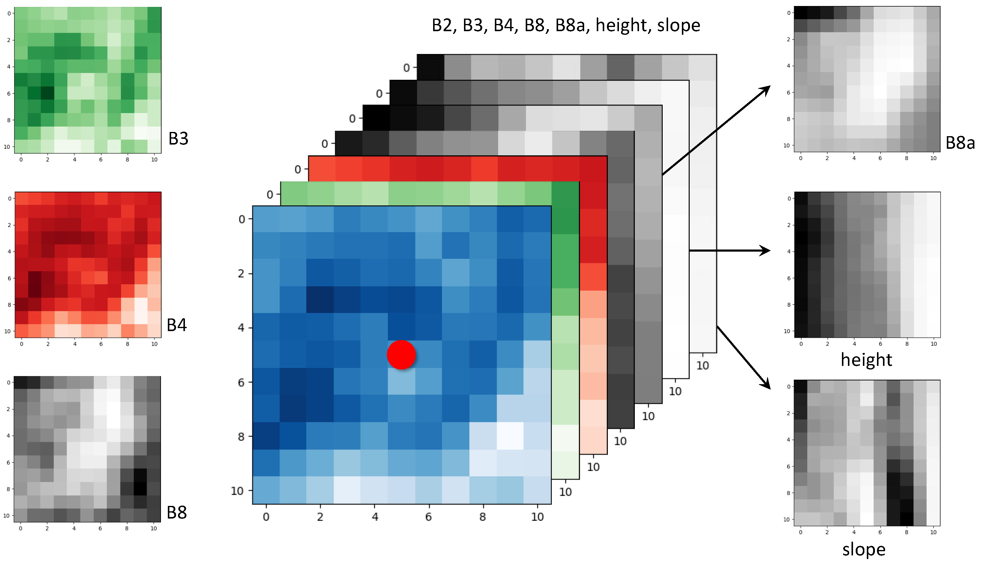
To produce the inputs, we matched the Sentinel-2 data with the soil erosion data by cropping square tiles of length 11 pixels centred around the coordinate points where the soil erosion was measured by Landgræðslan, such that every pixel within the square was labelled according to the erosion class of the central point, as illustrated in
Figure 2. This process was followed for each of the bands of interest, so that we had a set of 11 by 11 pixel tiles per band for each location. The DEM slopes and height data were also cropped to the same 11 by 11 pixels shape and centred on each location with a soil erosion measurement, where each pixel had a resolution of 10 m, matching the spatial resolution of some of the bands of interest.
Each tile was then checked to remove those with blank data (black regions of null pixel value), those with the same pixel value across the entire tile and those that are not of size 11 by 11 pixels. The coordinate systems were all converted into EPSG:3057 coordinates for consistency.
This resulted in a dataset that consisted of:
10,040 Sentinel-2A tiles of 11 by 11 pixels size across all 10 bands, spanning data collected between 2 July 2019 and 24 September 2021, and with a resolution of 10 m (resampled from a resolution of 20 m to 10 m as required),
742 DEM-based 11 by 11 pixel tiles representing height values in metres, with a resolution of 10 m per pixel, equivalent to 110 by 110 m pixels,
742 DEM-derived 11 by 11 pixel tiles representing slope values in degrees, with a resolution of 10 m per pixel, equivalent to 110 by 110 m regions,
553 datapoints in geopackage format with soil erosion classification between 0 (not eroded) and 5 (highly eroded),
from which we created our training set. The reason for the greater number of Sentinel-2A tiles per band than the number of DEM height and slope tiles is due to the overlapping of satellite images, such that multiple images cover the same region.
Lastly, we removed the duplicate Sentinel-2 observations of the same objects (regions) from the dataset to prevent bias from entering the model, resulting in 487 distinct objects. In any case, given the noisy data we had to work with, this was insufficient to create a strong, accurate model, so we split the pictures into single pixels and regarded the pixels as little pictures representing 10 by 10 m regions for the classifier to learn to classify. This resulted in a training set of 58,927 samples.
The resulting dataset was somewhat imbalanced across the 6 classes of soil erosion, as can be seen in
Table 1. Class 0 has fewer samples than any other class, which we take into account with stratification during the training process. Since the imbalance is small (i.e., the largest ratio between classes is approximately 2.4:1), we do not apply sampling techniques to create an evenly distributed dataset. The imbalance in the dataset is a reflection of the current distribution in erosion level of Iceland. There are fewer regions in Iceland with minimal risk/level of erosion compared to regions that are somewhat to severely eroded.
2.2. Algorithms
We trained three different machine learning algorithms to recognise the 6 different levels of soil erosion identified in the previous section: an SVM model, a RF model and an MLP model.
We applied a stratified
k-fold approach for cross-validation to ensure that the models were trained with a balanced training sample despite the imbalance present in our full dataset. The training, test and validation sets were randomly sampled from the full dataset provided as input to the models, following an 60:20:20 split, respectively. Each model was trained to predict the soil erosion severity of specific regions of Iceland based on Sentinel-2 satellite images in several height, slope and the calculated NDVI of each region in multiple wavebands. The training data used for each model was randomly sub-sampled from the training data we detailed in
Section 2.1.4.
For both models, we applied k-fold cross-validation with to detect signs of overfitting. As the training set was not well-balanced, we adopted a stratified approach to splitting the training and testing data, and used a stratified k-fold approach for cross-validation, which ensures the training and testing distributions reflect the distribution of the complete dataset. We set aside of the original dataset for testing purposes, which amounted to 47,141 training samples and 11,786 samples.
2.2.1. Support Vector Machine Model
The Support Vector Machine classification algorithm is a supervised machine learning technique that works by determining the hyperplanes—also known as decision boundaries—that best discern among the data categories. The hyperplanes that maximize the distances between them and the closest data points within each category they separate are the best-fitting ones. The SVM algorithm will find n-dimensional hyperplanes for a training set with n features. For our classification problem, we chose to start with the SVM algorithm because it is faster and performs better with smaller training sets than neural networks do.
Using the SVM algorithm that is included in the
scikit-learn Version 1.1.1 library [
43], the SVM model was constructed in Python 3. A radial basis function kernel was used as it produced the best results. We tested model performance across a wide range of values for the parameters
C and
, which control the margin of error for the decision boundaries and the similarity radius for data points in the same class, respectively. We tested values between
and
for
C, and between
and
for
. Within these intervals,
and
were the values that produced the highest accuracy without being either too small or too big (as to avoid overfitting and maximise performance at the same time).
2.2.2. Random Forest Model
The Random Forest algorithm is an ensemble learning algorithm that works by fitting independent decision tree classifiers to sub-samples of the training dataset, then combines the output of the decision trees to arrive at a single classification. The RF approach is suited to a training set of noisy data, such as satellite image data, as it tends to reduce variance in the output classification by combining the result of multiple decision tree classifiers.
The RF model was built in Python 3, using the RF algorithm available within the
scikit-learn Version 1.1.1 library [
43]. We used 125 estimators (decision tree classifiers) for our model, a figure we arrived at after experimenting with the number of estimators, ranging from 25 estimators to 200, and finding that the highest accuracy was produced with 125 estimators.
2.2.3. Multilayer Perceptron Model
An MLP is a class of feedforward artificial neural networks composed of multiple layers of perceptrons or nodes. The simplest form of an MLP consists of three layers of nodes: an input layer, a hidden layer and an output layer, where each node is a neuron with a non-linear activation function, and information is fed only in the forward direction from the input layer through to the output layer.
We ran numerous experiments on different architectures for the model before settling on a 4-layered model, which consists of an input layer with 256 nodes, 2 hidden layers with 128 and 64 nodes respectively, and an output layer with 6 nodes to match the number of classes in the problem. MLPs are suited for classification problems and are very flexible, and their relative simplicity compared to other neural network architectures allows them to be used as a baseline point of comparison with other models.
In contrast to the normalisation approach we followed to produce the training data for the SVM and RF models, we chose to use a min–max scaling technique to normalise the satellite data, the height data and the slope data before feeding them in to the MLP model for training. For each value in a given feature column of the training data, we used the following simple formula to perform the min–max scaling,
where
is the scaled value,
X is the original value, and
and
are the minimum and maximum values of the original feature column, respectively. This method of scaling places the data into a fixed range between 0 and 1, and was done to prevent the occurrence of different scales for different features as well as large input values, which negatively impact performance for deep learning models. We performed the scaling on each of the satellite band values, the height values and the slope values. The NDVI values were not re-scaled as they are by definition normalised to the range
. This scaling was tested for SVM as well; however, it led to a loss of accuracy for that model.
For our loss function, we used categorical cross entropy as it is specifically suited to our multi-class classification problem. For activation functions, we used the ReLU (Rectified Linear Unit) function for both the input and hidden layers, and the SoftMax function for the output layer. The optimiser chosen was the RMSprop optimiser with a learning rate of . We ran the training over 500 epochs, with 5 cross-validation folds, and with a batch size of 64.
The MLP model was trained in Python 3, using the Keras software library. The code was executed on Google Colaboratory, which provides free access to GPUs that were required for training the model.
3. Results
3.1. Model Performance Metrics
The overall accuracy achieved by the SVM model with and was . In all of our cross-validation runs, there was little variation in the overall performance of the model. The F1-scores and precision for each soil erosion class ranged from to , while the recall ranged from to , indicating that the vast majority of each class is correctly being identified by the model and when the model predicts that a sample is of a particular class, it is highly likely to be correct. The classes with the lowest F1-score and precision were classes 2 and 3, while class 3 had the lowest recall. The best scoring class across all three metrics was class 5.
The overall accuracy achieved by the RF model was , and again, there was little variation in performance across all cross-validation runs. The F1-scores and precision for each soil erosion class all ranged from to , while the recall ranged from to . The lowest F1-scores occurred for classes 2 and 3, class 2 had the lowest precision and class 3 had the lowest recall. The best scoring class across all 3 metrics was again class 5.
The performance of the MLP model is significantly lower than that of the SVM and RF models. It achieved an accuracy of , which exhibited only small variation across all the k-folds. The model performed significantly worse in precision, recall and F1-score for class 3 than for other classes, while class 5 exhibited the highest precision, recall and F1-score, consistent with the performance of the SVM and RF models. Unlike the other two models, the MLP model did not show worse performance in identifying class 3 samples compared to other classes. It achieved higher precision, recall and F1-scores for class 2 compared to classes 0, 1, 3 and 4.
We trialled a range of different architectures for the MLP model and evaluated their performance in order to identify the best performing MLP configuration. Specifically, we experimented with different layer numbers, different node numbers in each layer and the use of dropout layers to minimise overfitting.
The training and testing accuracies obtained with different model depths are shown in
Table 2. Our results demonstrate that despite increasing the depth of the MLP architecture and the number of nodes in each layer, the accuracy does not increase much. Where training accuracy is under 0.90, we can assume the model was underfit. Where the training accuracies were high, the testing accuracies were not able to exceed 0.80. Interestingly, extending the model to five layers (three hidden layers) only marginally improved the testing accuracy, despite the number of extra nodes available. Deeper models would likely be affected by overfitting.
Table 3 shows the impact of including drop out layers to a three or four layer model architecture, where the input layer has 256 nodes, the first hidden layer has 128 nodes and the second hidden layer (if applicable) has 64 nodes. Dropout layers prune preceding layers by removing nodes randomly to reduce the overfitting to the data, which we hypothesised may improve the testing accuracy compared to the training accuracy. The results shown in
Table 3 indicate that the inclusion of drop out layers did not improve the testing accuracies measured for each MLP configuration, and largely resulted in a decline in testing accuracy if more than
of nodes were affected in each layer. However, for the instances where
drop out layers were applied, the training accuracy was reduced as the number of drop out layers increased, which led to a reduction in the discrepancy between the training and testing accuracies. For drop outs that exceeded 10%, the testing accuracies declined along with the training accuracy. These accuracies and standard deviations were calculated across 10 cross-validation folds.
The above results suggest that the MLP architecture is not well-suited to this particular training set. We selected the simplest architecture that produced the highest testing accuracy for comparison with SVM and RF, resulting in the mentioned 4 layer arrangement.
Since there is a small imbalance in the training data used to develop the models, we also calculated Cohen’s
statistic, defined by the formula
to validate the other performance metrics we obtained.
is the overall model accuracy and
is the hypothetical probability of an agreement with ground truth values by random chance, which we can calculate by summing the probabilities of predictions randomly agreeing with ground truth values for each class, over all classes.
This is an alternative metric used to determine the agreement between model predictions and ground truth values that takes into account class distribution imbalances in the training data [
44]. Specifically, it compares the measured accuracy with the probability of agreement with ground truth if predictions were done by random chance.
has a range between
and 1, where 0 represents the amount of agreement that can be expected from random chance, and 1 represents perfect agreement between the ground truth and the model predictions.
We find that Cohen’s statistic reaches for the SVM model, for the RF model and for the MLP model. This means that the SVM and RF models’ predictions have reached very strong agreement with the ground truth classes, while the MLP model has relatively weak agreement.
The key performance results for the SVM, RF and MLP models are displayed in
Table 4. The accuracy reported is the overall accuracy achieved when using the models to predict on the test set, while the
k-fold accuracy is the average overall accuracy (with standard deviation) obtained during cross-validation across the 5 folds reserved for validation during training. The macro recall, precision and F1-score are the unweighted averages of the recall, precision and F1-scores achieved for each class.
3.2. Visual Representations
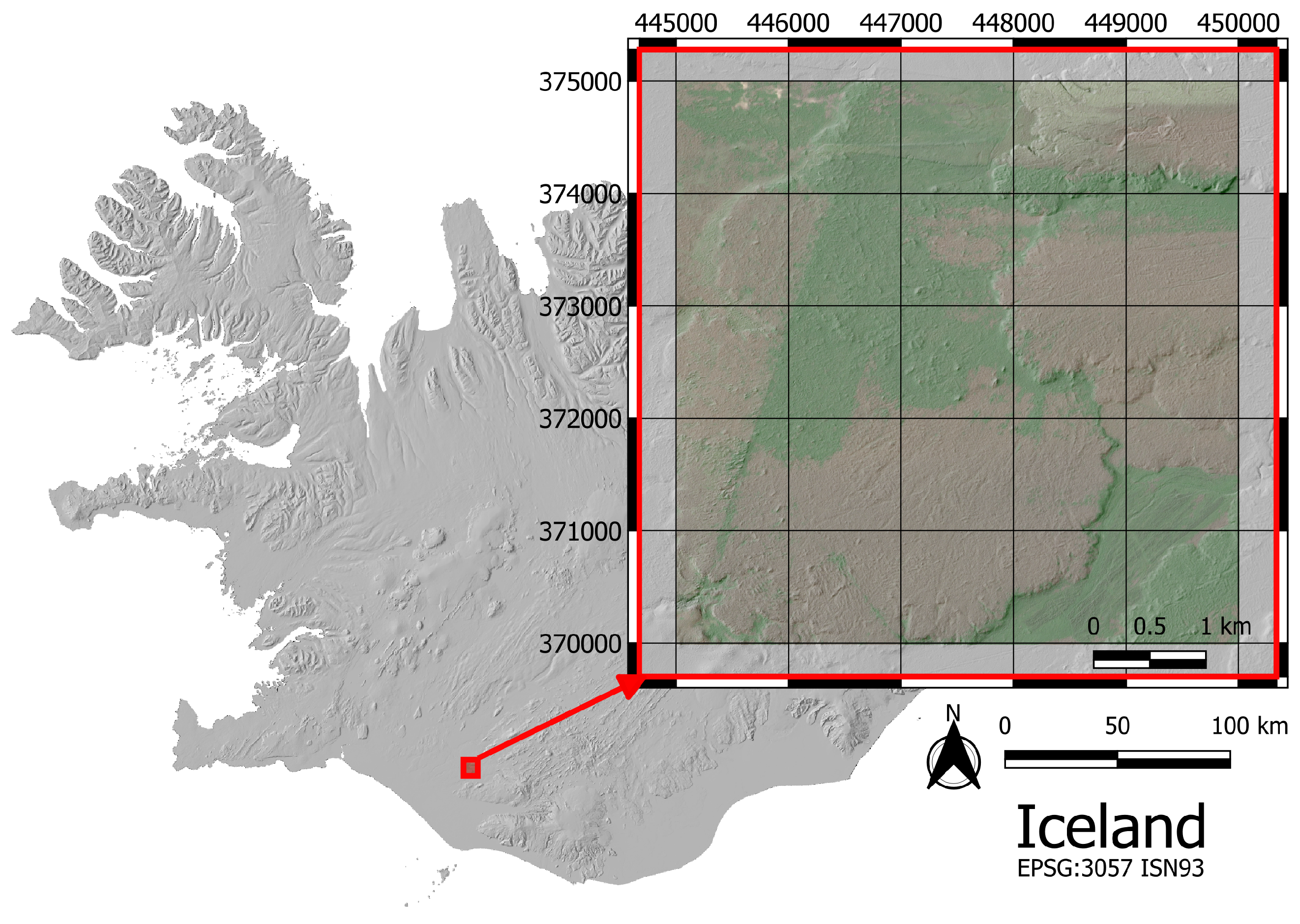
For illustrative purposes, we selected a small region to visualise the predictions for soil erosion levels made by the models, shown in
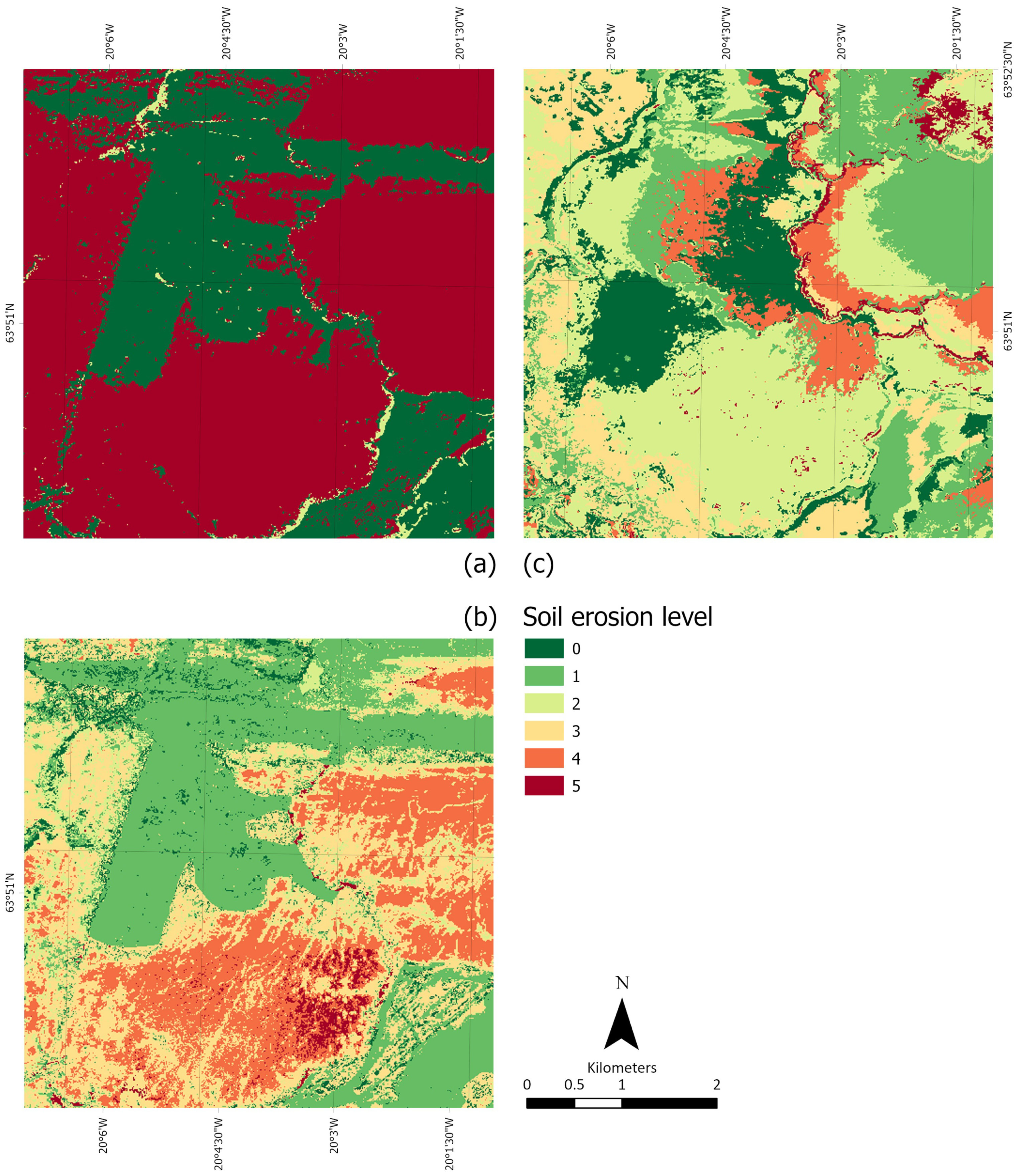
Figure 3. The predictions made by each model are displayed in
Figure 4. The erosion risk level is color-coded so that dark green represents Class 0 (very low erosion risk) and dark red represents Class 5 (high erosion risk).
There is significant disagreement in the predictions made by each model. The SVM predictions are only partially consistent with what we expect of the underlying geography of the test region. For example, parts of the vegetation areas marked by green in the test region image were assigned an erosion risk level of 4, which is not expected for vegetative land. We also find that the predictions for the elevated areas at the bottom and mid-right of the test region seem to bleed across to the vegetative regions surrounding them, despite the fact that these land types are quite different in nature. This is in contrast to the RF and MLP predictions, which appear to assign different soil erosion risk levels to the distinct regions. The SVM predictions are also quite varied within each distinct region. The vegetation section in the middle of the test region is classed into three different levels of erosion risk. The boundaries between these different classifications match small changes in the land that are observable in the test region, which suggests that these small changes in land characteristics were enough to cause the SVM model to assign different classifications to them, while the RF and MLP models were more robust to these small changes. Furthermore, these variations within distinct regions are not always continuous variations. For example, in the elevated land on the mid-right side of the test region, the SVM model shows variation from Class 1 to 2, and then Class 2 to 4, while within the vegetation region in the middle of the test region, we observe Class 1 transitioning directly into Class 4.
The RF model predictions exhibit far better matching with the underlying test region geography, and display a more continuous variation in classification of erosion risk wherever variations occur. However, the predictions are somewhat grainy in nature, which may be due to noisiness in the training dataset. The model predicts a low level of soil erosion risk for the vegetative patches and a medium to high risk of erosion for the elevated land, as expected.
The MLP model predicts a highly uniform level of soil erosion risk across each distinct sub-region. Although it predicts a low risk of erosion for the vegetation patches, the level of risk it assigns is lower than what the RF model assigns. Due to the lack of subtlety and variation in its predictions, we can only say that it generally agrees with the RF predictions in distinguishing between high risk and low risk of erosion depending on land type. The model fails to distinguish between more subtly different levels of erosion risk. The model we trained does not appear to be as sensitive to these subtle changes in features that the RF model is sensitive to, while the SVM model could potentially be too sensitive.
This is not surprising as the testing accuracy we obtained for the MLP model was only ; it is clear that the MLP model was underfit. In contrast, the SVM model achieved a very high testing accuracy, but when applied to an unseen patch of land, its predictions did not match well with expectations. This is indicative of a model that was overfit to the data we trained it on. Out of the three models, the RF model exhibits the best performance in predicting level of soil erosion risk.
3.3. Dependence of Erosion Risk on Height, Slope and NDVI
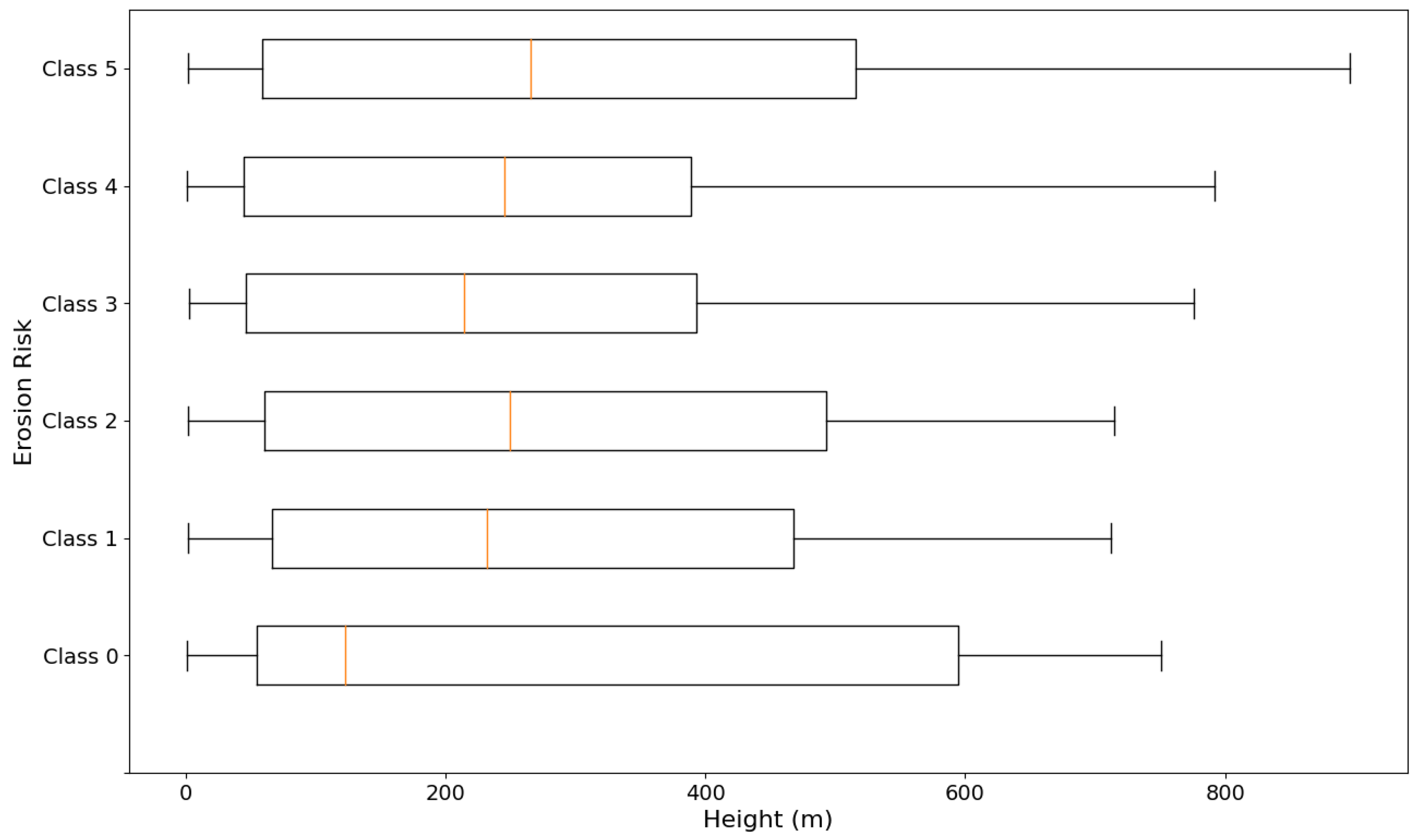
To test whether the risk of erosion within a region is correlated with its height, slope or NDVI, we calculated and plotted box-and-whisker distributions for each of the above characteristics, separated by erosion risk class and using all samples in the dataset described in
Section 2.1.4. Our results are displayed in
Figure 5,
Figure 6 and
Figure 7.
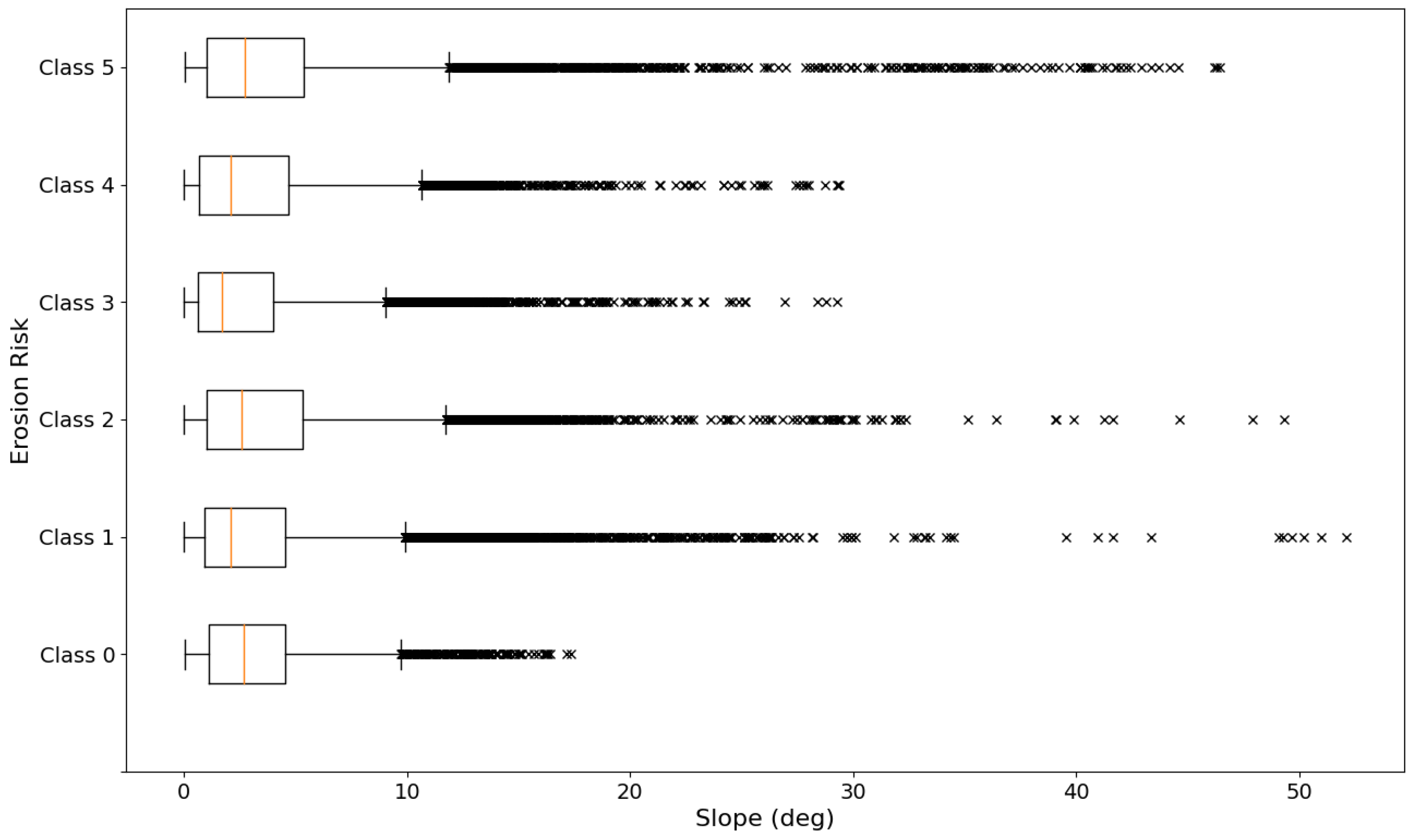
The box-and-whisker plots can be understood as follows: the median is indicated by the central orange line within the box, the box marks the values within the interquartile range (), the whiskers mark the values for and , and the crosses represent the values that lie outside the range , which may be considered outliers depending on the distribution.
Our results show that there is no clear correlation between height or slope and level of erosion. Within each erosion class, the distributions are very similar. The regions of greatest height (>800 m) all have the highest level of erosion, but otherwise there is no preferred soil erosion class at any height range. There is a small indication that a steeper area is more likely to be severely eroded than flatter areas; we observe that Class 5 contains many more regions that have a slope of >30 degrees than any of the other classes (including classes 1 and 2), while all regions within Class 0 have slopes under 17 degrees. However, classes 1 and 2 contain some of the steepest regions within the dataset, and neither the whiskers nor the medians of the slope distributions shift towards higher slope values with increasing erosion level.
These results indicate that while there is a theoretical motivation for a correlation to exist between soil erosion and height/slope, any such correlation is not clearly visible in the data, perhaps due to other contributing factors that more strongly impact soil quality.
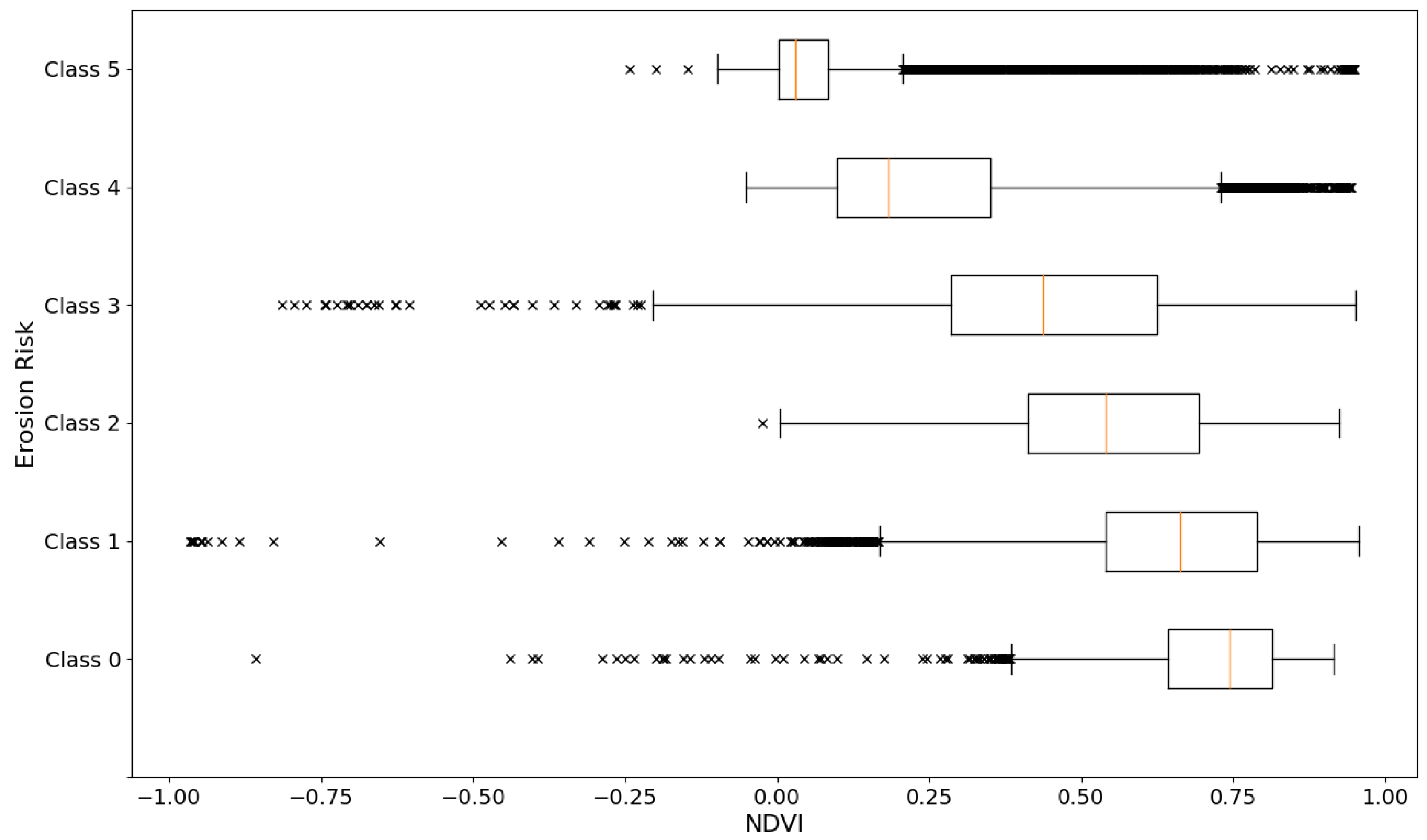
On the other hand,
Figure 7 shows that NDVI value is negatively correlated with level of erosion risk, as expected. The risk of erosion rises with decreasing median NDVI (
for Class 0 and
for Class 5. In the classes representing highest risk of erosion, the majority of samples have NDVIs closer to 0. Similarly, within the classes representing lowest erosion risk, the bulk of samples have NDVIs above 0.50. Out of all of the classes, the NDVI seems to be best at differentiating regions of severe erosion risk (Class 5), since the distribution within this class is fairly narrow and the vast majority of NDVIs occur below 0.25. As the samples within all other classes are more broadly distributed and there is considerable overlap in NDVI values between two or more these classes, the NDVI is less effective at distinguishing between them, particularly if its value falls between 0.25 and 0.75.
Interestingly, there are more NDVI values within Class 1 than Class 0 that fall between 0.75 and 1, so an NDVI in this range has greatest probability of being part of Class 1, rather than Class 0. There is even a small chance that a region with NDVI close to 1 is actually severely eroded, as class 5 contains some possible outliers that go against the general trend of low NDVIs.
Since vegetation is expected to reflect NIR wavelengths while absorbing red wavelengths of light, and therefore produce higher values of NDVI, it is not surprising that the higher values of NDVI are more likely to be classed as very low to moderate erosion risk. The fact that regions of moderate to high erosion risk can also exhibit higher values of NDVI suggests that there are other geographies other than vegetation that reflect NIR while absorbing red light, or that some vegetative regions are at risk of erosion.
4. Discussion
The results presented in this paper demonstrate that machine learning models are capable of accurately predicting level of soil erosion risk in Iceland based on satellite observations of the regions of interest and height and slope information. We find that the SVM and RF models achieve very high accuracy, precision and recall when tested on samples from the original training dataset, and the level of performance per class is quite consistent across all classes. In contrast, the MLP model achieves a relatively low accuracy, precision and recall.
The visual maps of the model predictions in
Section 3.3 show that despite the high performance of the SVM model as measured on the testing set, the quality of its predictions on the test region is far lower than that of the RF model. This suggests that the SVM model does not generalise well to unseen data, and is certainly overfit to the training data. This is consistent with expectations, as the SVM algorithm tends to be sensitive to noise and outliers. As we observed in
Figure 4, subtle and small differences in the land characteristics can cause the model to assign different risks of erosion to otherwise similar areas. Based on our observation, this is the main reason of over or underfitting the models. On the other hands, from soil science point of view, relying on just two topographic layers for soil erosion modelling does not make sense and thus layer significance in this case will not affect the model development and performance improvement. The RF algorithm does not have the same weakness, as it is an ensemble technique that relies on the averaging out of many independent classification models. This leads to both higher prediction accuracy and smaller likelihood of overfitting to meaningless noise. The SVM algorithm does employ regularisation principles to prevent overfitting, but it remains less robust to noise than RF. This is supported by other studies that have shown that RF outperforms SVM [
45], particularly as it is fairly insensitive to overfitting where there is high data dimensionality and potential multicollinearity [
46].
The predictions of the MLP model on the test region are also poor, but this is primarily due to underfitting by the MLP model rather than overfitting. However, there is another possible cause relating to how the min–max scaling was performed. For the test region, we used Equation (
1) to perform our scaling, which is consistent with how the training data was scaled prior to training the MLP model. However, the scaling factors used to scale the test region data and the original training data may be significantly different, due to the fact that the training data consists of pixels from hundreds of regions while the test region data consists of pixels from only the test region. The minimum and maximum values of both datasets may differ significantly, and result in a less accurate representation of the MLP model’s predictions on the test region. Identifying a suitable global minimum and maximum independent of the input data, by which to perform the min–max scaling, may result in a better set of predictions, though these predictions would still be affected by the low predictive power of the model.
The poorer predictive power of the MLP model could indicate that the general MLP architecture is not well-suited to the training data we used to train it, especially as changing the specific configuration of the MLP model did not significantly increase the testing accuracy. If a deep learning approach is preferred for this problem, then a Convolutional Neural Network (CNN) may be a better choice. Alternatively, the MLP model may train better if the data is kept as full 11 by 11 pixel tiles rather than split into individual pixels.
Another likely factor contributing to the lower accuracy and generalisability of the SVM model and the underfitting of the MLP model could simply be an excess of noise in the original training set, in the form of inaccurately classified pixels. The approach we used to create the training set required splitting the original 11 by 11 pixel tiles, each of which was labelled under a single class. Splitting the tiles into individual pixels and treating each pixel as a single data sample may have introduced a significant proportion of inaccurately labelled pixels into training, since the original 11 by 11 pixel tiles are very unlikely to all have the same ground truth level of soil erosion risk. The most accurately labelled pixels would be the ones closest to the centre of the 11 by 11 pixel tiles, while the pixels at the edge may be off by one (or more) class(es).
The fact that the RF model predictions (and to an extent, the SVM model predictions) are quite grainy may also be due to the inaccurately labelled pixels in the training set, particularly as the ‘grains’ seem to appear within areas where the predicted class differs by one. However, since RF is expected to be quite robust to noise, this may not be the primary contributing factor. A more likely explanation may be the model’s sensitivity to the DEM data inputs; there is a chance that the grainy pattern is correlated with the DEM data. Applying a smoothing filter to the predictions can address the issue of graininess to improve the classification.
Despite the issues highlighted above, our results indicate that there is strong potential for using remote sensing combined with machine learning to identify land areas that are at risk of soil erosion. Our results support the recommendation of RF over SVM and MLP for predicting the level of soil erosion risk based on satellite observations. Although CNNs have been shown to exhibit better performance than SVM and RF in remote sensing applications [
47,
48], our results demonstrate that RF is still a good choice of model for such applications. The RF algorithm is capable of producing highly accurate predictions and has the advantage of being much more easily implementable and interpretable than deep learning algorithms. For certain problems in remote sensing, such as where training samples or computing resources are limited, or where simplicity and training speed are important, SVM and RF models may be better options than deep learning models.
To further improve the models, particularly the performance of SVM, it is most important to reduce the number of inaccurately labelled pixels in the training set, perhaps by changing our pixel by pixel approach to use smaller tiles, or by implementing a weighting that varies with distance from the centre of the tile. Moreover, in our present study, we have only utilised one spectral index (the NDVI) out of many indices that may provide additional predictive power to our models. It is worth experimenting with other indices in future to enhance their performances.
The extension of our most viable algorithm to a nationwide prediction study would result in the first soil erosion map of the country since the map from RALA of 1997, published in [
4] and then later in [
49]. A comparison would be of great interest.
Regarding conducting an ecosystem assessment of our results, this is challenging task since it would demand a more extensive analysis of historical data. Historic classification is limited by the quality and availability of historic imagery, and long term monitoring of ecosystem properties throughout the Arctic from satellite information is still largely absent to this date [
50], particularly in Iceland. Quantitative analyses such as the ones described in this study can open a new avenue for the understanding of landscape change dynamics.
Furthermore, the ecosystem function can differ greatly between land cover types, suggesting that further input parameters may need to be added in order to draw conclusions about the interdependence of the processes involved in long term observations. As a case in point, our study has focused on the NDVI index, which is susceptible to trends in precipitation-evapotranspiration. The presence of surface water absorbs light in the near infrared, thereby reducing this index while landscape drying increases it [
51].
Changes in ecosystem type also alter interactions between climate and permafrost, which may evolve in response to climate change. Accurate prediction of the permafrost carbon climate feedback will require detailed understanding of changes in terrestrial ecosystem distribution and function, which depend on the net effects of multiple feedback processes operating across scales in space and time [
52].
Further improvement could also come from testing topographic derivatives other than slope and purely elevation values, such as aspect (due to wind erosion), texture, terrain ruggedness, wetness indices, etc.
5. Conclusions
The aim of this study was to investigate the suitability of using ML algorithms with satellite imagery as inputs to assess the risk of soil erosion in Iceland. Specifically, we evaluated the performance and potential of an SVM model, a RF model and an MLP model in classifying soil into one of six classes of erosion risk.
To conduct the study, we created a training set composed of cropped geo-referenced and atmospherically corrected Copernicus Sentinel-2 images of Iceland (normalised satellite image arrays in the Bands 2, 3, 4, 8 and 8a) and Arctic DEM-derived heights and slopes. We also calculated the NDVI index as an additional input to the models, and showed that it is correlated with soil erosion risk, while height and slope are not. For our ground truth values, we used measurements of soil erosion in Iceland provided by the Icelandic Soil Conservation Services.
We found that both the SVM and RF models achieved very high testing accuracies, F1-scores, precisions and recalls, based on evaluations completed on a reserved portion of the training set, while the MLP model performed comparatively worse on the same measures. The SVM model achieved an average accuracy of , the RF model achieved an average accuracy of and the MLP model achieved an accuracy of , across the five folds. However, when testing the predictions of the models on an unseen region in Iceland, we found that the neither the SVM model nor the MLP model performs as well as the RF model. The SVM model predictions do not match the underlying geography as well as the RF model predictions, and the model generally exhibits too much sensitivity to minor and irrelevant changes in the land characteristics. In contrast, the MLP model predictions match the underlying geography reasonably well, but the model was not sensitive enough to changes in land features that were linked to soil erosion.
We conclude that the SVM model is overfit and does not generalise well to unseen data, while the MLP model is underfit, suggesting that the underlying model architecture is not suited to this problem. Out of all the models, RF exhibited the best performance and appears to generalise well to new data. The performance of the RF model shows that simpler machine learning algorithms can still produce accurate classifications for soil erosion and may be viable alternatives to more complex and resource-intensive implementations such as deep learning models.
The appropriateness of erosion concepts commonly employed in model structures is still questionable. Despite the fact that physical processes of detachment, transport, and deposition in overland flow are well recognized and have been widely incorporated within erosion models, the experimental procedures to test conditions when processes are occurring concurrently have only recently been developed. Our initiative of using machine learning approaches therefore proves to be a promising alternative for erosion prediction in which it overcomes obstacles in parametrization, calibration, and validation processes that are often considered to be the main difficulties while applying conventional models.
The goal of the research described in this work intends to produce a reliable, widely applicable, and cost-effective method to classify Icelandic soils into various categories of erosion risk. A proof of concept that, once engineered, could be easily expanded and applied to other Arctic regions, such as Greenland and Canada.

 ,
, 

