What Are We Missing? Occlusion in Laser Scanning Point Clouds and Its Impact on the Detection of Single-Tree Morphologies and Stand Structural Variables

Abstract

Laser scanning has revolutionized the ability to quantify single-tree morphologies and stand structural variables. In this study, we address the issue of occlusion when scanning a spruce (Picea abies (L.) H.Karst.) and beech (Fagus sylvatica L.) forest with a mobile laser scanner by making use of a unique study site setup. We scanned forest stands (1) from the ground only and (2) from the ground and from above by using a crane. We also examined the occlusion effect by scanning in the summer (leaf-on) and in the winter (leaf-off). Especially at the canopy level of the forest stands, occlusion was very pronounced, and we were able to quantify its impact in more detail. Occlusion was not as noticeable as expected for crown-related variables but, on average, resulted in smaller values for tree height in particular. Between the species, the total tree height underestimation for spruce was more pronounced than that for beech. At the stand level, significant information was lost in the canopy area when scanning from the ground alone. This information shortage is reflected in the relative point counts, the Clark–Evans index and the box dimension. Increasing the voxel size can compensate for this loss of information but comes with the trade-off of losing details in the point clouds. From our analysis, we conclude that the voxelization of point clouds prior to the extraction of stand or tree measurements with a voxel size of at least 20 cm is appropriate to reduce occlusion effects while still providing a high level of detail.

1. Introduction

Laser scanning has revolutionized the ability to quantify single-tree morphologies and stand structural variables, e.g., [1,2,3]. By using terrestrial laser scanners, the structures of trees and stands can be recorded more quickly and accurately than with conventional methods [4]. During the last several years, this technology has opened new opportunities for environmental scientists and foresters [5]. The aboveground structure of a forest is one of the key features of forest ecosystems and especially influences which ecosystem services are provided by the system. For example, Gough et al. [6] found a significant influence of the forest structure on forest productivity, and Bauhus et al. [7] observed its effects on forest stability and resilience. Moreover, the forest structure is related to biodiversity, e.g., [8,9], and to microclimate regulation, e.g., [10,11].

For forest inventory purposes, single-tree morphologies, such as the tree height and diameter at breast height, can be derived from laser scanner data, e.g., [12]. One advantage is that such classic variables can be measured faster and more efficiently with laser scanners. However, it is also possible to quantify characteristics that have hardly been measurable to date. The technique has also enabled more precise and efficient ways of measuring crown morphologies, such as the height of the maximum crown projection area, the maximum crown projection area, the crown volume and the crown surface area. These are of interest for several tree physiological relationships (e.g., [13]). Jacobs et al. [14] showed, on the basis of laser scan data, that drought stress affects the crown size and tree height.

Lidar-based scanners are currently the dominant solution for outdoor mobile mapping [15]. For many forestry-related questions, laser scan data are either collected from the ground or from the air. When scanning from the ground, there are basically two different approaches: terrestrial laser scanning (TLS) and mobile laser scanning (MLS), also often called handheld personal laser scanning (HPLS). In TLS, the three-dimensional point cloud is achieved through single scans with a fixed viewpoint [16] or by combining multiple single scans [17]. Since multiple scan locations are required to accurately capture the forest structure and to reduce occlusion, the method is time-consuming and costly. MLS, on the other hand, is faster and therefore more cost-efficient [18]. This technology uses an inertial measurement unit to determine the position of a laser while the laser takes distance measurements of its surroundings.

When scanning from the air, the scanner is attached to an aircraft, for example, an unmanned aerial vehicle (drone) or a light aircraft (airborne laser scanning (ALS)). ALS has a high area coverage but, presently, still has a lower point cloud resolution than terrestrial/mobile laser scanning from the ground. Additionally, difficulties arise in obtaining detailed tree structures due to canopy occlusion [19]. Mobile laser scanners, on the other hand, are well suited for scanning forest stands and individual trees with a high level of detail, e.g., [20,21].

Aerial scans and ground-based scans are limited to a single perspective of the forest, either from above or below the canopy. This necessarily results in an occlusion effect, e.g., [22,23]. It remains unclear how much information is missed by being restricted to one perspective and how this affects tree and stand structural variables derived from laser scans. Most likely, the amount of information missed due to occlusion depends on the distribution of biomass in space. Especially dense stands can be assumed to be susceptible to either approach [24].

Beech (Fagus sylvatica L.) is a tree species that forms very dense stands due to its high shade tolerance and pronounced development of shade leaves [25]. Such canopies can act as shields against laser beams even at lower stand heights. Spruce (Picea abies (L.) H.Karst.) also forms dense canopies but loses its needles in lower stem sections under dense stand conditions due to the lack of light. In both cases and for both species, laser scanners are likely unable to detect the upper crown due to occlusion when scanning from the ground during the vegetation period. In winter, on the other hand, beech trees shed their leaves, whereas spruce trees do not lose their needles. Due to increased visibility in winter, the accessibility of beech canopies with laser beams from the ground should be better for beech than for spruce in the leaf-off period.

To obtain stable estimations of structural and morphological variables, the issue of occlusion is often addressed by reducing the spatial resolution of the point cloud based on so-called voxelization, e.g., [26,27]. Voxelization has the potential to compensate for occlusion and the spatial variation in the point cloud density with distance from the scanner to a certain degree, depending on the voxel size. However, voxelization is also accompanied by a loss of detail in the point cloud and an increase in space-filling estimates. While voxels should not be too small to ensure reduced occlusion, they should also not be too large to prevent severe losses in resolution. A voxel size of 10 or 20 cm side length is often chosen as a compromise [22,27,28].

In this study, we intended to address the issue of occlusion in mobile laser scanning from the ground by making use of a study site with the possibility of scanning a forest stand from below and above. The aim was to quantify the potential loss of information and to detect the pattern showing where information is lost and how the loss changes with different voxel sizes. To do this, we scanned forest stands (1) from the ground only and (2) from the ground and from above by using the crane experiment KROOF [29]. We also examined the seasonal effect for beech by scanning in the summer (leaf-on) and winter (leaf-off) seasons.

The hypotheses of this work were driven by two assumptions. First, the effect of occlusion (information loss) in deciduous species is stronger in summer than in winter because the leaves reduce the visibility of the upper parts of the crown (seasonal comparison). Second, there is occlusion in the tree crown when scanning only from the ground. Even under the best conditions (no leaves), an occlusion effect remains due to the lack of perspectives of the objects of interest from above (methodological comparison). The specific hypotheses were:

Seasonal comparison

H1. 

For beech, the occlusion effect leads to significant differences in single-tree morphologies when comparing summer to winter ground scans; for spruce, there are no significant differences.

H2. 

For beech stands, the occlusion effect results in a significant difference in stand complexity when comparing summer to winter scans; for spruce, there is no significant difference.

Methodological comparison

H3. 

For single trees, the occlusion effect leads to smaller values for canopy morphologies of all trees (e.g., lower height and smaller crown volume) when scanned only from the ground.

H4. 

For stands, the occlusion effect results in an underestimation of the stand structural variables when scanned only from the ground.

H5. 

For stand-specific variables, the occlusion effect is reduced in importance as the resolution of the data decreases (voxel size increases).

2. Materials and Methods

2.1. Study Area

The study area was located in the Kranzberg Forest (48°25′09.8″N; 11°39′39.8″E) in the southern part of Germany, about 35 km northeast of Munich [30]. Within the forest, there is the unique Kranzberg Forest Roof (KROOF) experiment on an area of 0.5 ha [31]. The KROOF experiment was originally designed as a drought stress experiment. In addition to water retention by roofs, a canopy crane had been installed at the KROOF experimental site (Figure 1c). This allows research to be conducted at heights of up to 45 m. In this study, this crane was used to complement the ground scans with scans from above the forest canopy.

The mixed stand primarily consists of pure tree groups of Norway spruce (Picea abies (L.) H.Karst.) and European beech (Fagus sylvatica L.) trees that were planted in 1951 ± 2 y and 1931 ± 4 y, respectively [29]. These two tree species are among the most common tree species in Germany, with forested area shares of 25% for spruce and 16% for beech [32], and are coniferous and deciduous, respectively. According to inventory data for the KROOF site, beech trees had a height of about 28 m and spruce trees had a height of about 32 m on average [31]. The average diameter at breast height (dbh) was about 29 cm for beech and about 35 cm for spruce [31]. In total, there were 639–926 trees per ha with a stand basal area of 54.0–60.1 m²·ha⁻¹, a standing stem volume of 802–981 m³·ha⁻¹, and a mean periodic volume increment (1998–2016) of 19.4–26.3 m³·ha⁻¹·y⁻¹ [33].

2.2. Data Collection

Data were collected in the pure sections of spruce and beech stands. The two areas selected for scanning each had a size of 30 m × 40 m (1200 m²). The areas were scanned during two different seasons of the year, in summer 2020 (during the vegetation period, leaf-on for deciduous trees) and in winter 2020/2021 (leaf-off for deciduous trees). There was nearly no growth between summer and winter scans, and we can also exclude possible influences of the different treatments of the drought experiment. To record the plots, we used the ZEB HORIZON mobile laser scanner (GeoSLAM Ltd., Nottingham, UK). The ZEB HORIZON mobile scanner is able to scan objects up to a distance of 100 m from the scanning device using the time-of-flight principle and SLAM (simultaneous localization and mapping) technology (e.g., [34]). As a data collector, Velodyne VLP-16 multibeam LiDAR is embedded in the device. The wavelength of the laser was 903 nm, the scan rate was 300.000 points per second and the range noise was ±30 mm with expected system accuracies of 1–3 cm. Each scan followed the same predefined scanning procedure.

First, the specific areas (beech and spruce) were only scanned from the ground, following a predefined walking pattern (Figure 2a), further referred to as the “ground scan”. For the second scan, the same walking path was used as for the first scan (with otherwise identical conditions) but was then complemented by a canopy scan. To do this, the scanner was attached to the crane and moved up vertically over the top of the canopy (Figure 1) while operating. The crane was then set in motion horizontally by turning it clockwise and moving the scanner along the horizontal crane axis. This allowed the area to be scanned from above and below within one single scan (Figure 2b). This scan is further referred to as the “full scan”. The starting point of the scans was always the same. In total, 8 different scans were performed (2 plots (beech and spruce), 2 conditions (ground scan and full scan) and 2 seasons (summer and winter)). The scans were performed under optimal weather conditions (no wind, fog, rain, or frost).

2.3. Data Processing

The data collected by the mobile laser scanner were first processed using the manufacturer-specific software GeoSLAM HUB 6.1 [35], which means that actual SLAM registration was performed. This was carried out with the default software configuration, turning off any additional sharpening or filtering. After preprocessing, the individual scans were exported in the .laz file format. The R package “lidR” [36] was used to further process the exported point clouds. The point clouds were clipped to the specific tree collective (area size 30 m × 40 m). Ground points were then classified using the Ground Segmentation Algorithm [37]. With the Spatial Interpolation Algorithm (interpolation is performed using a k-nearest neighbor approach with inverse-distance weighting), the heights of the points were normalized. To reduce the amount of data, the point cloud was initially voxelized to a resolution of 1 cm (representative voxel size of 1 cm³). To ensure that the point clouds of the different scans overlapped exactly, they were aligned using CloudCompare software (version 2.11.3, cloudcompare.org, EDF R&D, Paris, France).

From the remaining point cloud, the point clouds of 20 single trees per species and scan were identified. Trees were then precut using the software LiDAR360 [38]. The tree segmentation algorithm used was developed based on the method described by Li et al. [39]. Each tree was manually postprocessed using Cloud Compare software for better quality. The full scan from winter was used as a reference for segmenting the same trees from the ground-based scans. By overlaying the single-tree point clouds, it was possible for each point to be assigned to the correct tree, even for scans that recorded very few points in the upper canopy.

From each single-tree point cloud, the following single-tree morphological variables were calculated: total tree height (tth), diameter at breast height (dbh), height of maximum crown projection area (hcpa), maximum crown projection area (cpa), crown volume (crvol) and crown surface area (csa). The dbh was determined using circular fitting (height range of 1.29–1.31 m) (R package “circular” [40]), and the height was obtained from the maximum z-value of each point cloud. The crown base was defined as the height where the horizontal cross-section of the crown first reached five times the base area of the tree. The maximum crown projection area (cpa) and corresponding height (hcpa) were calculated where a horizontal cross-section of 20 cm thickness reached its maximum value. The crown volume and crown surface area were computed using a convex hull around the remaining point cloud above the crown base (R package “geometry" [41]). All single-tree morphologies were calculated with a voxel size of 1 cm.

From each scan, we clipped six circular subplots with a radius of 5 m at identical points for stand structure analysis. For these subplots, we calculated the relative point counts in three-dimensional space, the Clark–Evans index and the box dimension, as described below. We calculated the change in the point counts with height relative to the respective maximum value (relative point counts). For this calculation, we cut 1 m thick horizontal slices from the point clouds and determined the number of points for each of them. For each height layer, the mean value for each of the 6 subplots was calculated. The largest mean value for the respective winter scans (ground scan and full scan) was defined as 100%, and all other values were calculated in relation to the largest value.

We used the aggregation index from Clark and Evans [42] to calculate the spatial description of the point distribution (CE index). The CE index is widely used to characterize forest structures, e.g., [26,27]. The CE index examines the horizontal distribution of objects for clumping or regularity. The calculated value theoretically ranges from 0 (strongest clumping, where all objects are at the same point) to 2.1491 (strictly regular hexagonal pattern). Aggregation values less than 1.0 indicate a tendency towards clumping, values around 1.0 indicate a random distribution, and values above 1.0 indicate a tendency towards a regular distribution. The calculation was performed with the R package “spatstat” [43]. Before the calculation, we projected the 1 m thick horizontal strata onto a plane by setting the z-value of each voxel to zero. Duplicate voxels were deleted. To avoid edge bias, Donnelly edge correction was applied [44,45].

The box dimension can be used as a measure of the structural complexity of forests [46] and is often used to differentiate different forest structures, e.g., [26,27]. It considers the density and three-dimensional distribution of objects at the same time. The box dimension was calculated based on specific subplot point clouds. We used the maximum tree height as the upper cut-off. The lower cut-off, which is the smallest box-edge length used in the box-dimension calculation, was defined as the respective voxel size tested (5–50 cm). We calculated the box dimensions for three horizontal forest strata of each 3D point cloud (1–12 m, 13–24 m and 25–36 m), as well as for the overall forest. Details on the box dimension can be found in Seidel [46] and Sarkar and Chaudhuri [47].

The relative point counts, the Clark–Evans index and the box dimension were derived for voxels of 5 cm (5 cm³), 10 cm (1 dm³), 20 cm (8 dm³) and 50 cm (125 dm³) edge lengths.

2.4. Data Analysis

To determine differences in the single-tree morphologies and metrics for the stand structure, we used the paired Wilcoxon rank-sum test with Bonferroni-corrected p-values, since the normal distribution and the homogeneity of variance could not be confirmed for all of the studied variables. The significance level of p < 0.05 was chosen for all statistical tests conducted in this study. All statistical procedures were performed using R 4.1.2 [48].

3. Results

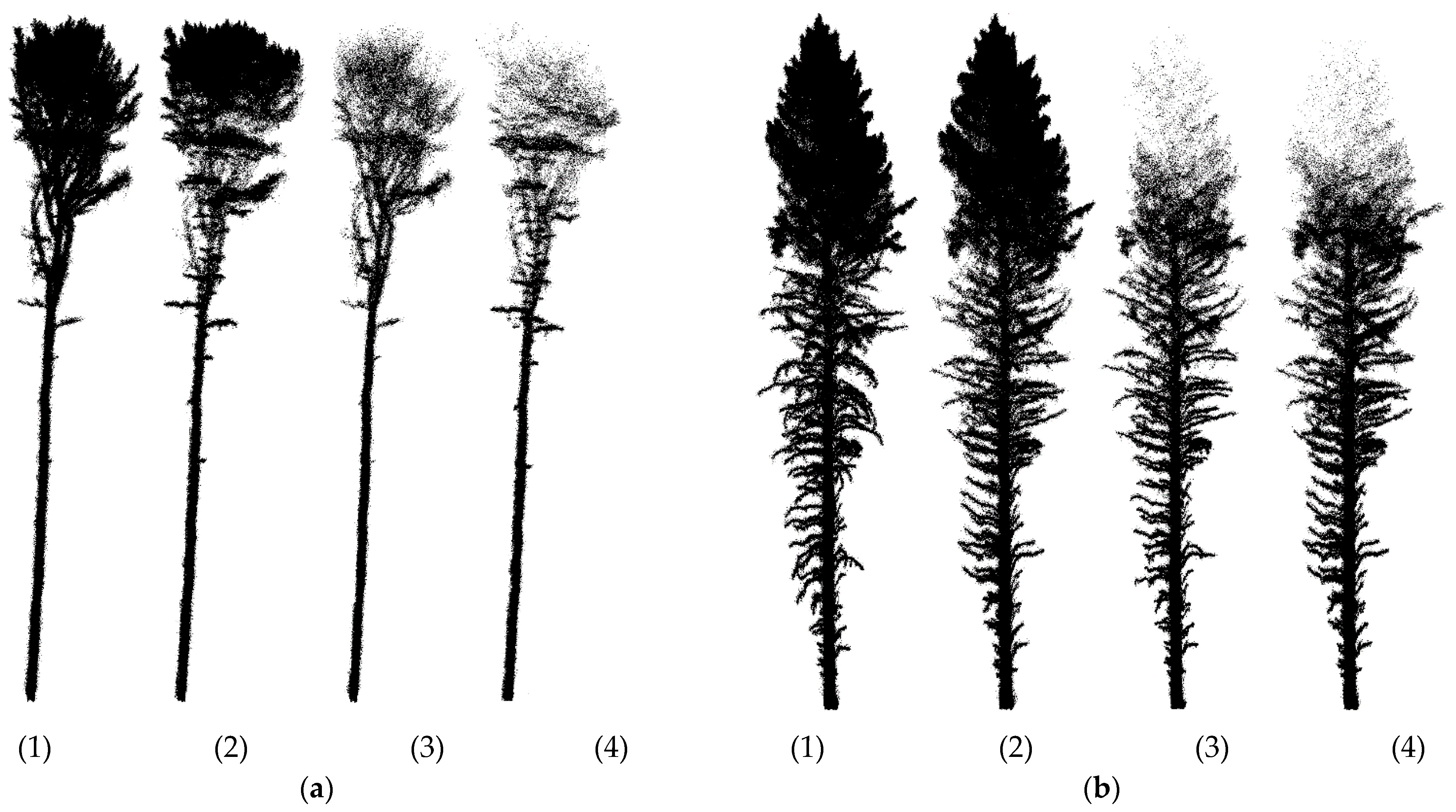
3.1. Visual Assessment of Single-Tree Point Clouds

Clear morphological differences between the point clouds of spruce and beech could already be detected visually at the single-tree level (Figure 3a vs. Figure 3b). These differences were apparent between the ground scans and the full scans (Figure 3(1,2) vs. Figure 3(3,4)). The point clouds of the ground scans (Figure 3(3,4)) lose much detail in the upper parts of single-tree crowns. Additionally, the effects of seasonality could be detected visually to a certain extent for beech, obviously less so for spruce: for the full scans, Figure 3a(1) shows a smaller, more narrow crown appearance in the winter, when there are no leaves, compared to the summer (Figure 3a(2)), when there are leaves on the tree. However, differences could also be detected between the seasons from the visual inspection of ground scans: when comparing Figure 3a(3,4), the point cloud density in the upper crown layer seems to decrease even more in summer compared to winter. Such differences could not be detected visually for spruce (Figure 3b(3,4)).

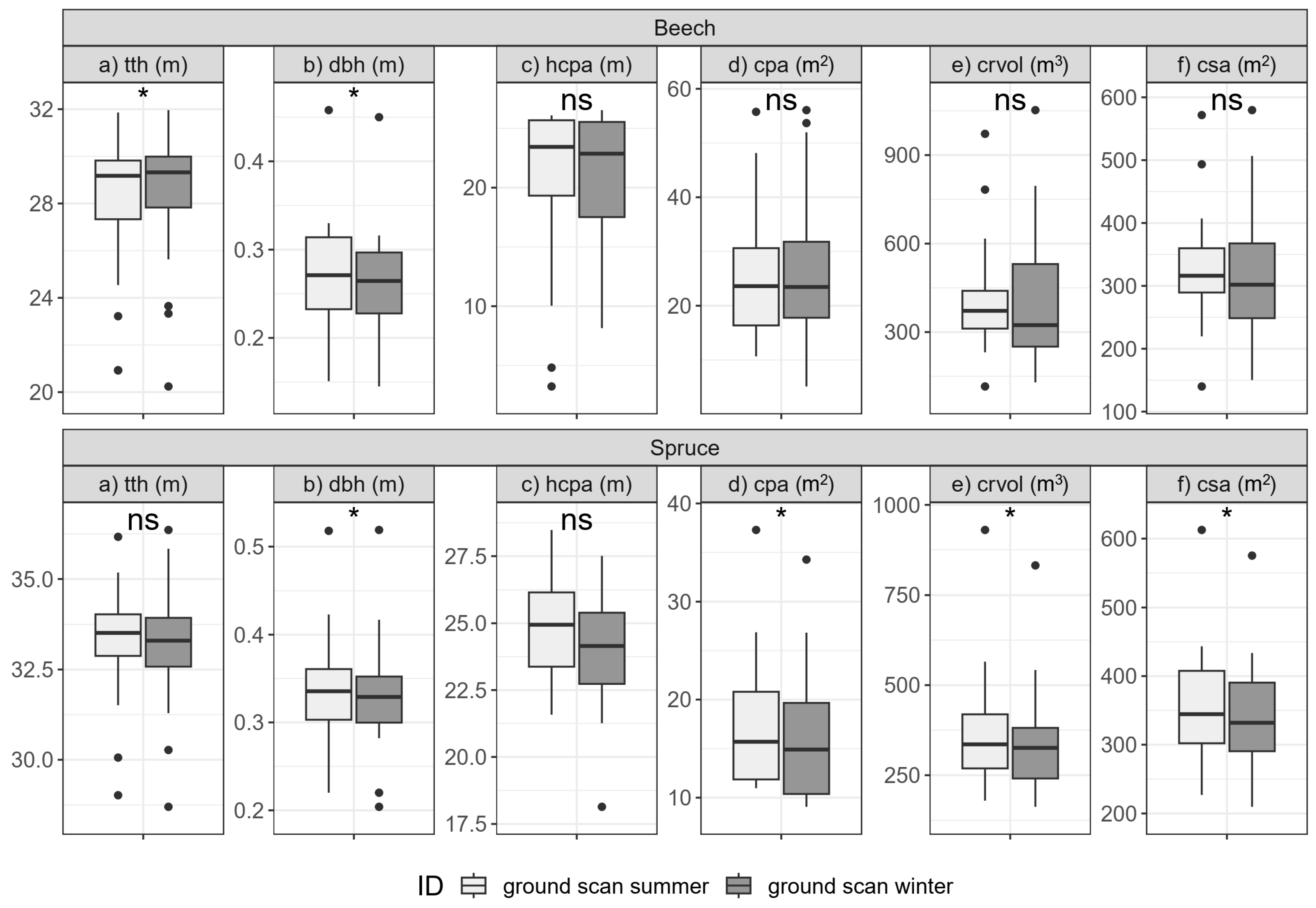
3.2. Seasonal Comparison

3.2.1. Single-Tree Morphologies (H1)

The seasonal comparison at the single-tree level only partly confirms the visual impressions of Figure 3, namely, that the single-tree morphologies in the respective scans differ depending on the season in which they were recorded (Figure 4). The overall differences were not very pronounced for the crown-related variables, which were derived from the part of the point clouds where the occlusion effect was most noticeable when scanning from the ground. Only the total tree height of beech trees was estimated to be slightly lower on average for the summer scans compared to the winter scans. Other crown-related variables were not significantly different for beech (hcpa, cpa, crvol, and csa, cf. Figure 4, Beech c–f). In addition to the total tree height, the dbh of beech trees was also significantly bigger in summer 2020 than in winter 2020/2021 (cf. Figure 4, Beech a; Table S1). We could also detect significant differences for spruce scans (bottom row in Figure 4) for the diameter at breast height, the maximum crown projection area, the crown volume and the crown surface area, which were all smaller on average in winter 2020/2021 than in summer 2020. No significant differences were found in the total tree height or the height of the maximum crown projection area. Table S1 shows the mean differences ± standard deviations between ground scans in summer and ground scans in winter for both tree species and whether the difference is significant between the species.

3.2.2. Stand Structure (H2)

Pronounced seasonal differences in stand structural complexity could be found for whole stands when comparing the winter and summer ground scans (Figure 5). The box dimension was significantly influenced by the seasonal effect. Across all height ranges of the point clouds, the values of the box dimension differed significantly. In addition, there were also species-specific differences. While the box dimension of spruce (Figure 5, bottom row) was always larger in summer than in winter, the picture was slightly different for beech (Figure 5, upper row). For beech, the box-dimension values from the winter ground scans were larger for the highest point cloud layer (25–36 m) compared to the summer ground scans. The largest values for the box dimension were found in the medium height range of 13–24 m for the stands of both species. The differences in the box dimension at resolutions of 10, 20 and 50 cm are shown in Figure S1. At these resolutions, the same trends seen at the 5 cm resolution are observed. However, these are not that pronounced. In particular, for beech, the pronounced difference in the 25–36 m height range at a 5 cm resolution becomes progressively smaller with reduced resolution.

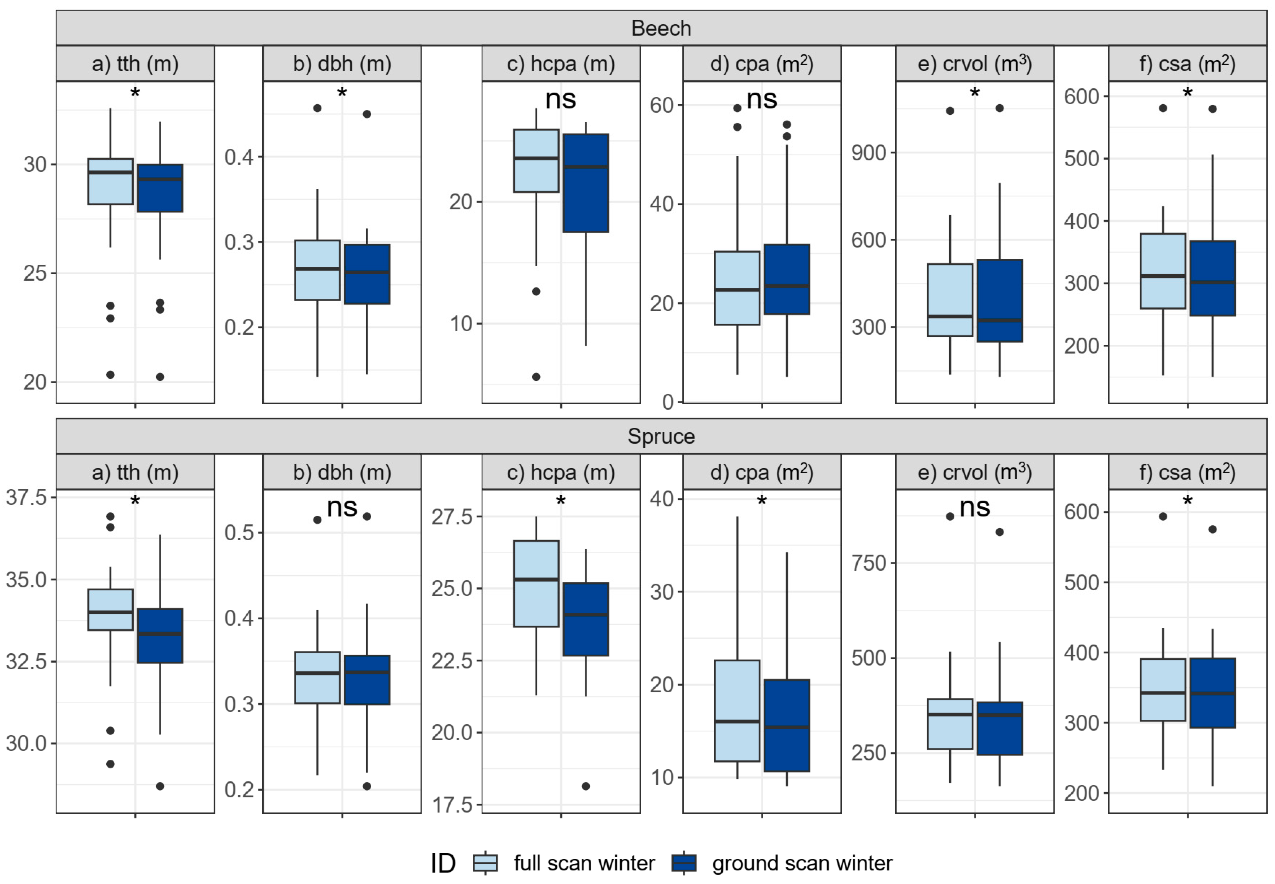
3.3. Methodological Comparison

3.3.1. Single-Tree Morphologies (H3)

The methodological comparison of the two scanning methods (ground scan and full scan) in winter, the optimal scanning season, shows differences in the single-tree morphologies (Figure 6). The resulting total tree height was lower on average when scanning from the ground (Figure 6, left column) for both tree species. The effect was more pronounced for spruce than for beech (

Table 1. Mean difference ± standard deviation between the full scan in winter and the ground scan in winter for beech and spruce (n = 20 for each species). The data are presented in absolute (abs.) and relative values (rel. in %). Listed are the single-tree morphological variables total tree height (tth), diameter at breast height (dbh), height of maximum crown projection area (hcpa), maximum crown projection area (cpa), crown volume (crvol) and crown surface area (csa). The p-value indicates whether the difference is significant between beech and spruce.

	Beech (abs.)	Beech (rel.)	Spruce (abs.)	Spruce (rel.)	p-Value
tth (m)	−0.30 ± 0.34	−1.04 ± 1.20	−0.74 ± 0.45	−2.19 ± 1.34	0.001
dbh (m)	−0.01 ± 0.01	−3.35 ± 5.02	0.00 ± 0.01	−0.18 ± 2.42	0.025
hcpa (m)	−0.88 ± 2.78	−4.00 ± 12.68	−1.24 ± 2.41	−4.94 ± 9.58	0.685
cpa (m2)	+0.43 ± 5.68	+1.59 ± 21.16	−1.12 ± 1.44	−6.42 ± 8.23	0.602
crvol (m3)	+4.85 ± 103.09	+1.22 ± 26.00	−3.88 ± 17.47	−1.11 ± 4.98	0.052
csa (m2)	−2.31 ± 41.29	−0.73 ± 12.98	−5.97 ± 13.31	−1.72 ± 3.84	0.445

). The same is true for the crown surface area. Furthermore, for beech, the derived diameter at breast height was smaller and the crown volume was larger for the ground scans compared to the full scans (Table 1). For spruce, significant differences were especially found in the height of the maximum crown projection area and the maximum crown projection area itself (Figure 6, Spruce(c,d)).

When analyzing the differences in the morphological variables of both species, they were surprisingly similar (Table 1). However, besides the dbh, one especially significant difference could be found between the species: namely, the total tree height underestimation for spruce was more pronounced than that for beech. For all other variables, the p-value is above the significance level of 0.05, and the effect size is hence in a similar range for both species.

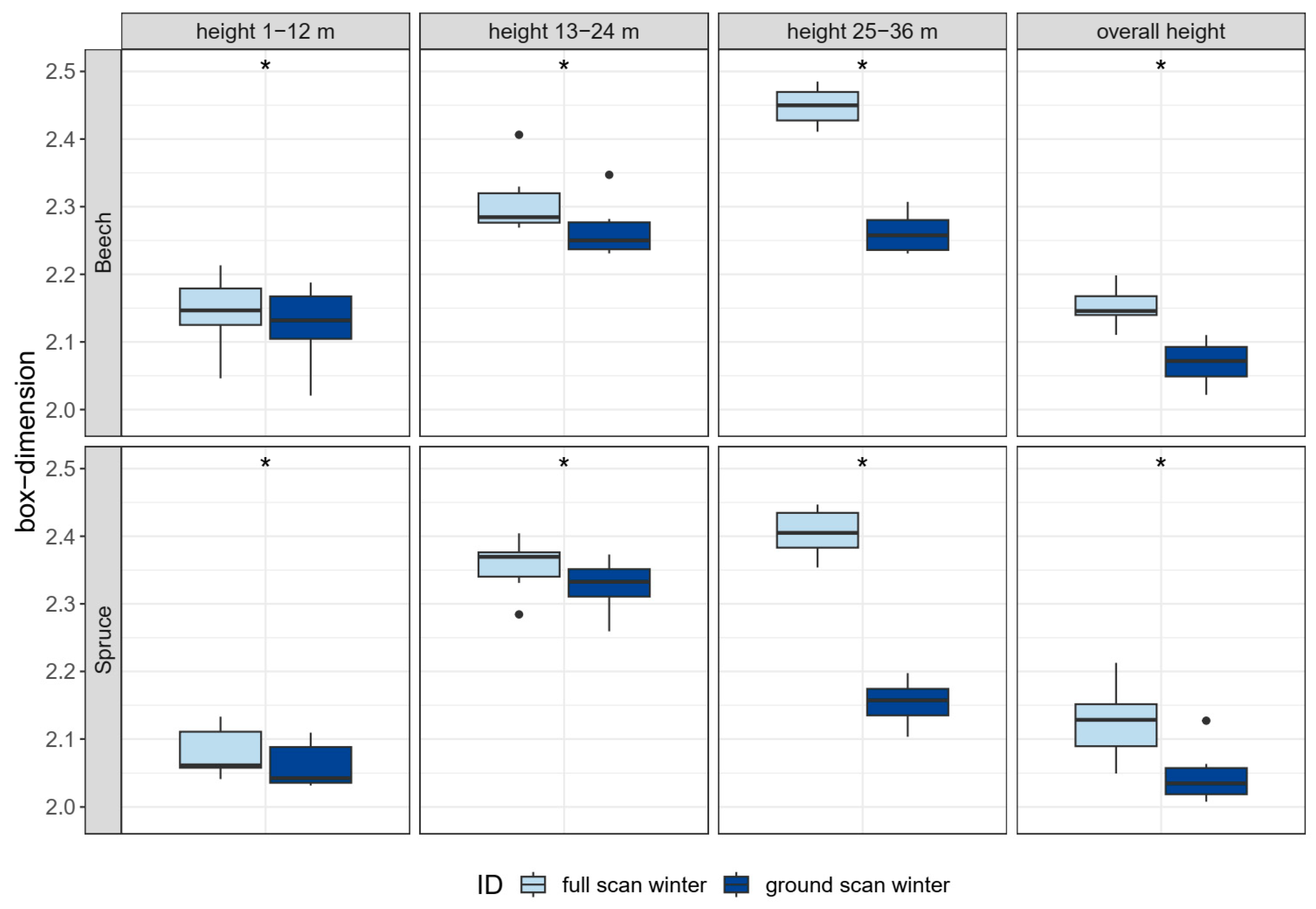
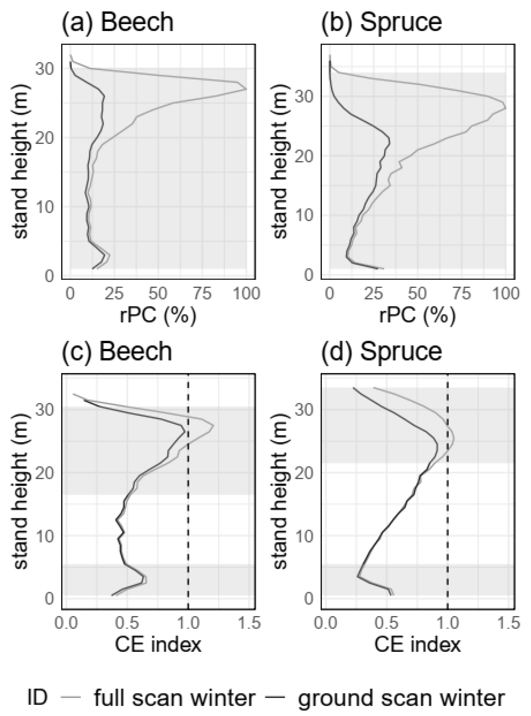
3.3.2. Stand structure (H4)

The methodological comparison at the stand level shows that the values of the box dimension were larger in the full scan compared to the ground scan for both tree species (Figure 7). The values in the lower two height ranges for both tree species were close together (1–12 m and 13–24 m) (first two columns in Figure 7). However, the differences were clearly greater in the upper height range of 25–36 m, where a lot of information on the structural complexity is lost. Here, the full scans result in a significantly higher box dimension, with the effect being slightly larger for spruce than for beech. Additionally, for the full point clouds, the box dimension is significantly larger for the full scans compared to the ground scans (last column in Figure 7).

An analysis of the relative point counts with height also showed that significantly fewer points were recorded over almost the entire height spectrum when scanning from the ground compared to the full scan (Figure 8a,b). The difference was particularly apparent in the crown regions of the stands for both tree species. At heights where the maximum number of points (100%) for the full scans were recorded (27 m for beech and 28 m for spruce), they only accounted for 16% for beech and 8% for spruce on a relative scale at the corresponding heights. The heights at which the maximum number of points were reached were lower in the ground scans than in the full scans for beech and spruce.

Similar trends were found for the CE index, but the trends were more consistent (Figure 8c,d). The CE values for both tree species were highest in the crown area, indicating that the points were more regularly distributed in space there. When comparing the ground scans to the full scans, the scans in the lower height range hardly differ from each other. For the higher parts of the stand, the CE values diverge. For the full scans, the regularity in the distribution pattern further increased in the higher canopy layers (gray lines in Figure 8c,d). The difference starts to become significant at a height of 17 m for beech, (Figure 8c) and at 22 m for spruce (Figure 8d). Additionally, for the ground scans, the CE index for both tree species remains below 1.0 over the entire height range.

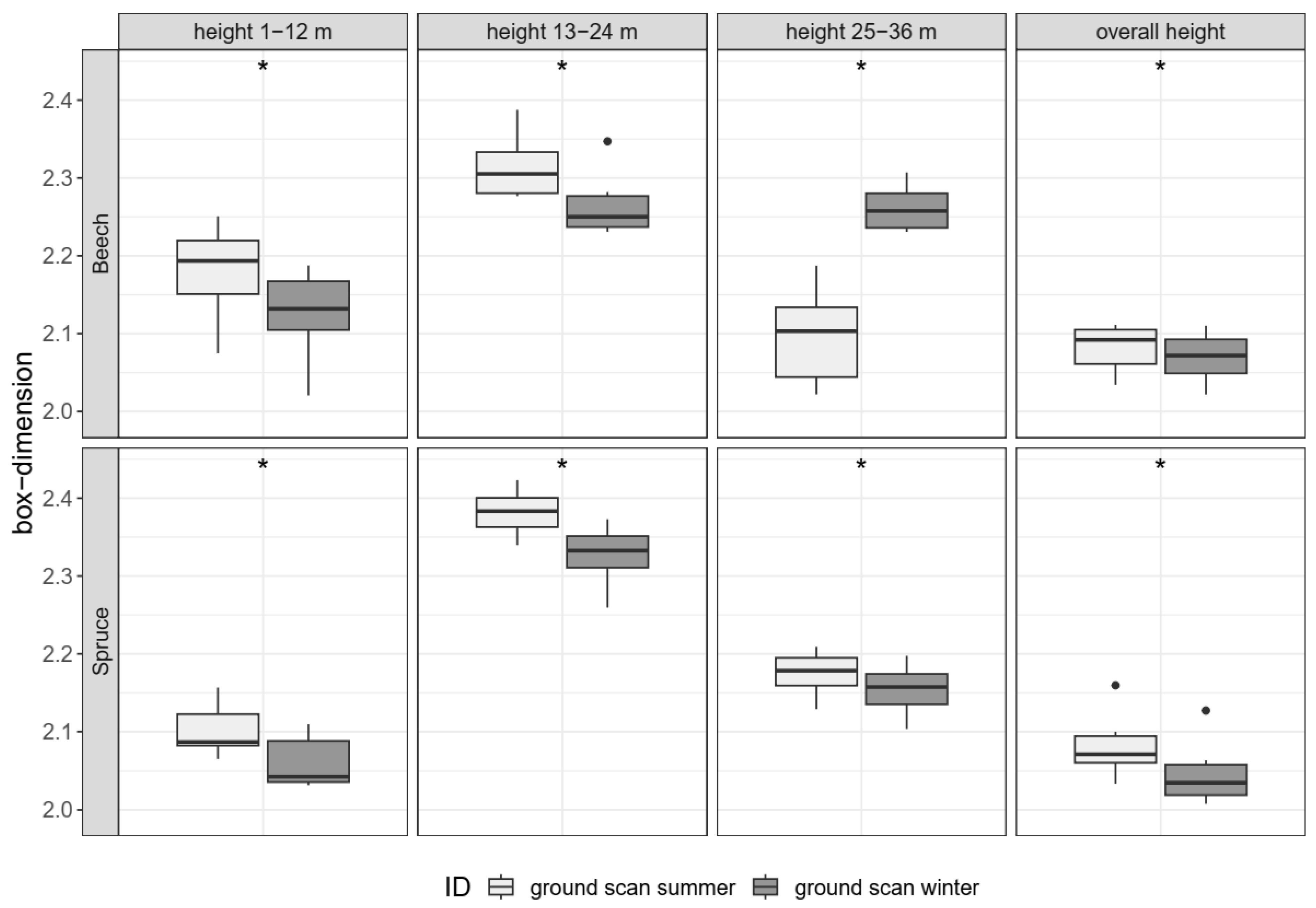
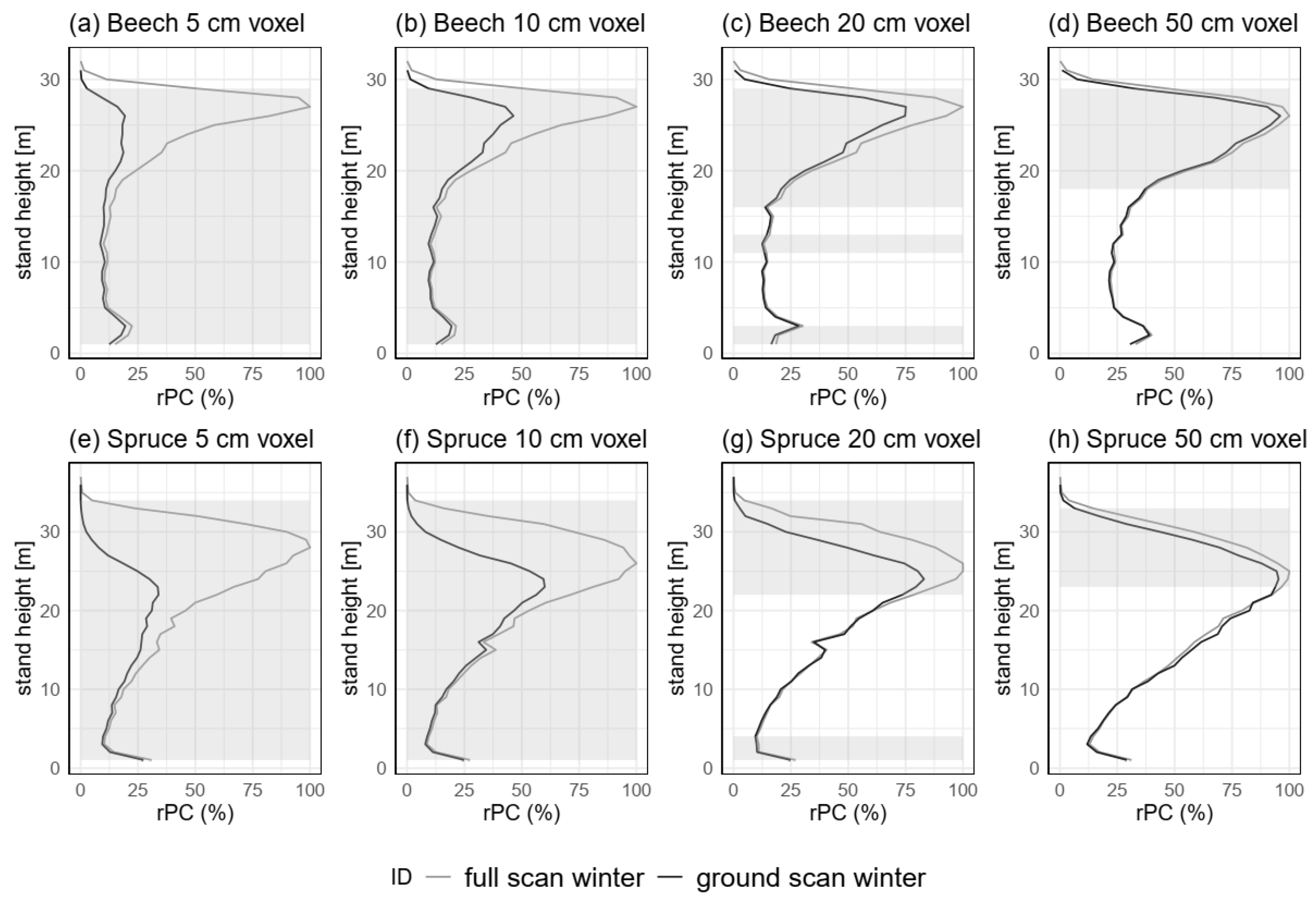
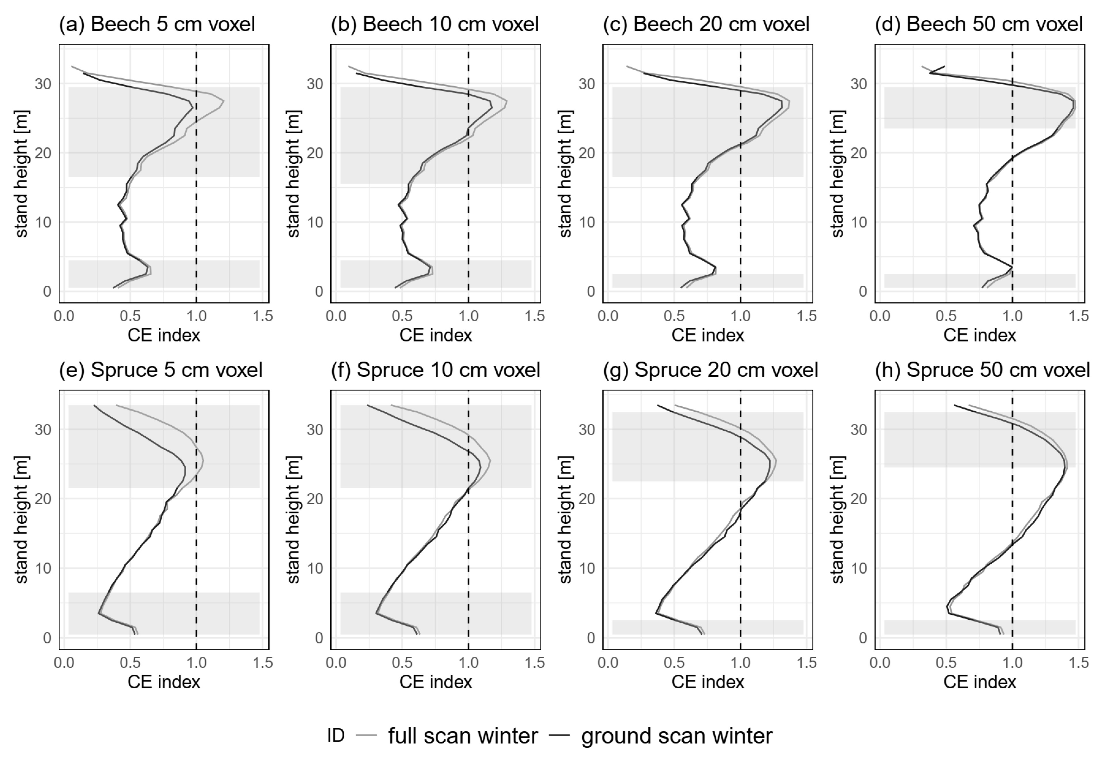
3.3.3. Spatial Resolution (H5)

The observed loss of information in the ground scan point clouds (e.g., Figure 7 and Figure 8) decreases with decreasing spatial resolution, i.e., with increasing voxel size. In Figure 9, this is exemplified by the relative point counts. When increasing the voxel size from 5 cm to 50 cm, the trend lines of the ground and full scans become increasingly similar; i.e., for a voxel size of 5 cm, the number of points in the canopy was underestimated, which becomes less and less pronounced from 10 cm voxels through 20 cm voxels to 50 cm voxels. This was true for both tree species. However, even at 50 cm voxels, significant differences in the canopy range remain between the point counts of the ground scans and full scans.

For changing resolutions, the CE index (Figure 10) shows a similar picture to rPC (Figure 9), namely, that an increasing voxel size decreases the divergence between the trend lines of the ground and full scans. However, the initial differences between the CE values were not as pronounced to start out with, meaning that the CE values point in a very similar direction, even at a voxel resolution of 5 cm. In addition, the CE index values generally increase in each height section with increasing voxel size. The arrangement of voxels in space becomes more and more regular due to the effect of increasing the voxel size. The height threshold, above which the tendency towards a regular distribution is indicated, shifts slightly downward with decreasing spatial resolution. At the same time, the maxima of the respective curves shift upward (Figure 10a–d). For spruce, it was similar (Figure 10e–h).

The differences in the box dimension at resolutions of 10, 20 and 50 cm are presented in Figure S2. With a lower resolution, the same trends seen with the 5 cm resolution are observed. However, the significance range differs and is generally not as pronounced.

4. Discussion

4.1. Seasonal Comparison

In the seasonal comparison (summer and winter), occlusion effects could be detected in the data for single trees and whole stands (Figure 3, Figure 4 and Figure 5), as assumed with H1 and H2. The tree heights of beech were especially affected by the time of scanning (Figure 4 and Table S1). They were lower for beech in summer, most likely because the dense canopies of beech trees prevented sufficient laser beams from reaching the top sections of the trees on average. Beech is a tree species with high crown plasticity [49]. As a result, beech forms a dense canopy and develops many green leaves in the lower part of the stem during the vegetation period due to its higher shade tolerance, e.g., [50]. Spruce also forms dense canopies but loses its needles in lower stem sections under dense stand conditions due to the lack of light [25,51]. For beech, the greater photosynthetically active mass in the lower canopy results in a greater reduction in the laser beam compared to spruce.

However, we could not detect any differences in the other crown morphological variables of beech (hcpa, cpa, crvol and csa). Here, we would have expected larger deviations, because the ground scan in summer was strongly thinned out in the upper crown area, and the crown architectures were no longer easily recognizable. An explanation for why no differences appeared could be that the full scans from winter were available as orientations when the trees were manually cut out from the point cloud. With the full scan from winter, the points could be assigned to the correct tree. However, the upper crown area was still only very sparsely populated with points, and without the full winter scan reference, it would have been unclear which tree they belong to. However, overall, the three-dimensional space of the single-tree point cloud was occupied in such a way (cf. Figure 3a(4)) that the algorithms used calculated very similar single-tree morphologies, although the occlusion was pronounced.

We did not expect any differences for spruce, because growth was already complete when the summer scan was performed at the end of August 2020, and the winter scan was performed before the start of the 2021 growing season. So, no major growth should have taken place between the summer and winter scans. Initially, we could not detect such differences visually since this species does not shed its needles in winter (Figure 3b(3,4)). However, the results show that even more single-tree morphological variables differ from each other than for beech (Figure 4). This could indicate that the noise of the laser scanner in combination with the algorithm used to calculate the metrics affect the morphologies of the individual trees in such a way that even two identical scans in a row result in slightly different values. The differences are small, but still significant (Figure 4 and Table S1). MLS scans are known for their comparatively high level of noise [52]. The accuracy of MLS scans at a distance of 5 meters is about 20 times lower than those produced by TLS [53]. The range noise (noise along an axis perpendicular to the target) of the device used in this study is estimated to be around ±30 mm, according to the manufacturer [54]. Trzeciak and Brilakis [53] found that the range noise of the ZEB Horizon scanner was 40–50 mm at 40 meters. Based on these numbers, the scanner has an error of approx. +/−0.1% (4/4000 cm). The deviations we observed for the dbh measurement, for which we can exclude an occlusion effect, are on average 3.08% for beech and 1.04% for spruce in the seasonal comparison (Table S1) (methodological comparison: beech: 3.35%; spruce 0.18% (Table 1)). The deviations we determined are therefore larger than the specified range noise from Trzeciak and Brilakis [53] and are more in line with the findings of Hunčaga et al. [55] according to which the dbh could be determined with a maximum error of up to 4 cm.

At the stand level (Figure 5), the values of the box dimension (>2) for each season are within a plausible range for both tree species, e.g., [27,56,57]. Depending on the season (winter or summer), we found different values of the box dimension in both tree species. In the case of beech, this could be due to the foliage. It is also conceivable that environmental influences such as slight leaf shaking, which cannot be avoided, even when there is no wind, could additionally amplify the noise. Neudam et al. [20] and Guzmán et al. [58] also concluded that leaf-bearing trees produce more scattered point clouds than leafless trees. At the stand level, occlusion is particularly evident in the canopy layer of beech trees (Figure 5). The crown architecture is only captured to a limited extent in the summer scan, which is reflected by smaller values for the box dimension in the height range from 26 to 36 m (Figure 5, third column above). For the total stand (overall height), the values from the summer scan are, however, larger than those from the winter scan, which is consistent with the findings of previous studies, for example, by Neudam et al. [20]. Seasonal differences in the box dimension of spruce were not expected. We can only explain the deviations in our data as noise in the point cloud.

In summary, we found differences in single-tree morphologies and stand complexity for beech. However, contrary to our expectations, we also found such differences for spruce. Thus, we have to reject hypotheses H1 and H2.

4.2. Methodological Comparison

4.2.1. Single-Tree Morphologies

The comparison between the ground and full scans resulted in lower heights for both tree species when scanned only from the ground, as assumed in H3. This is most likely due to the more strongly pronounced occlusion effects of the crown in the ground scans (Figure 6a). The laser beams are blocked by the biomass, which means that the upper canopy sections are not fully detected. The very large number of laser beams was not sufficient to determine the same height in the ground and full scans for beech in winter conditions. In the case of spruce, as an evergreen tree species, this difference is greater than in the case of beech. Besides the evergreen condition of spruce, its pyramidal crown could play a role in this finding. In a dense stand, this crown shape makes it very difficult to detect the top of it. In the study area, the density of the trees was also very high (639–926 trees per hectare, standing stem volume of 802–981 m³·ha⁻¹). The visibility of the crown is therefore limited for the laser beams.

We expected the canopy morphologies from the ground scans to be smaller than those from the full scans because of the occlusion. In addition to some height values, this was also true for the height of the maximum crown projection area, maximum crown projection area and crown surface area for spruce. For beech, this was only true for the crown surface area. The crown volume, in contrast, was greater when scanning only from the ground. As with the seasonal comparison, we attribute this result, on the one hand, to the noise of MLS and, on the other hand, to the methods we used to calculate the tree canopy morphologies. For example, the convex hull method spans a relatively large hull around the crown. This in itself can result in relatively large changes in the derived quantities due to only a few differences in points in the point clouds [59], specifically for the crown volume. In combination with the noise, we therefore explain the differences as originating from this.

To what extent the deviations determined in this study are relevant for future studies depends on the research question and its accuracy requirements. Especially since traditional methods, such as vertex height measurements, are also associated with uncertainties [60], which can sometimes be larger, the MLS technique seems to nevertheless be a very suitable tool for determining single-tree morphologies. Overall, the differences in the single-tree morphologies were small, even though they were partly significant. Occlusion effects led to a systematic underestimation only for height, in the range of 1.04% for beech and 2.19% for spruce, regarding the methodological comparison.

4.2.2. Stand Structure

At the level of the stand structure, the methodological comparison for both tree species shows that the biomass in the canopy is not captured as well when scanning only from the ground (Figure 7 and Figure 8). This is reflected by lower proportions of points detected and by lower values for the CE index and the box dimension, especially in the canopy, as we postulated with Hypothesis 4. This is in line with our expectations that the reduced number of laser beams reaching the top canopy layers because of occlusion results in underestimations in this vertical range of the stands. There are also differences in the lower range, although both scans were performed in a direct temporal sequence (both scans were performed within one hour under the same weather conditions). Again, this must be attributed to inevitable noise in the data, e.g., during the SLAM processing itself, due to small wind gusts, etc. In the full scan, each object in the forest stand is scanned from far more different perspectives and distances than in the ground scan. Trzeciak and Brilakis [53] found that edges and corners become less and less recognizable as the distance to the object increases. In the full scan, the additional view from above likely led to increased blurring in object recognition during the SLAM procedure, and as a result, the noise in the full scans increased.

In summary, since not all canopy-related single-tree morphological variables were smaller when only scanning from the ground, we must reject Hypothesis H3. Hypothesis H4, on the other hand, can be accepted, since the ground scans underestimated the upper canopy layers, which significantly affected the stand structural variables.

4.2.3. Spatial Resolution

The problem of losing information in the upper canopy layers and underestimating these ranges could be overcome by increasing the voxel size, as we have assumed with Hypothesis 5 (Figure 9 and Figure 10). As the voxel size increases, the differences between the data sets (ground scan and full scan) decrease. However, even at a point cloud resolution of 50 cm, some of the differences remain in the point clouds between the full and ground scans. These were more pronounced for the relative point counts than the CE index. However, for the CE index, a reduction in spatial resolution resulted in larger values per height level. As a consequence, for example, when comparing the 5 and 20 cm resolution values for the CE index, the differences can reach orders of magnitude, which corresponds to the findings described in other studies between different forest types, e.g., in studies by Stiers et al. [26] and Willim et al. [27]. This underlines the importance of considering the spatial resolution of point clouds when comparing stand structural variables, whereby the characteristics and trends of the respective curves (e.g., the number of maxima and minima of each curve) are mainly maintained, which is again elementary for characterizing the structure of a stand. The choice of spatial resolution here resembles a typical trade-off system. To us, a voxel size of 20 cm seems to be an appropriate size to reduce the effect that occlusion has on the data and still provide enough detail at the forest stand level. The same conclusion was also made by Heidenreich and Seidel [21].

To compensate for the occlusion effect, one could introduce a correction factor across the vertical range of the stand. For studies where a high level of detail is required, it might be useful to combine MLS ground scans with drone scans to mimic the full-scan approach used here. Once the occlusion is determined for a stand type, it could be minimized with correction factors for other ground scans in similar stands. When transferring the results of this work to other forests, it should be considered that the performance of scanning devices depends on the environment, particularly illumination conditions, with sunlight reducing the scanner range [61,62].

Hypothesis H5 (occlusion is reduced as the resolution of the data decreases) can be accepted, since a reduction in the point cloud resolution also reduced the effect of occlusion on stand structural variables (i.e., box dimension, relative point counts and CE index). However, reducing the point cloud resolution also changed the range of the stand structural variables, which needs to be considered when changing the point cloud resolution.

5. Conclusions

By using a crane to produce full scans, we were able to quantify the occlusion effect, apparent in every ground scan, in more detail. The effect was pronounced in the canopy range of the stands. For single-tree morphologies, occlusion plays a role, especially when extracting single-tree point clouds from the entire point cloud. With only a single scan from below, beech trees could not be extracted accurately and comparably. The noise of the laser scanner in combination with the algorithms used to calculate the metrics affected the morphologies of the individual trees. Overall, we could not detect very pronounced differences in the crown-related variables. It is the nature of these variables that they are derived from the parts of point clouds where the occlusion effect is most noticeable when scanning from the ground. However, here, occlusion effects led to a systematic underestimation only for height, in the range of 1.04% for beech and 2.19% for spruce, regarding the methodological comparison.

At the stand level, a significant amount of point information was lost in the canopy range when scanning from the ground alone. Increasing the voxel size can compensate for this loss of information but comes with the trade-off of losing details in the point clouds. From our analysis, we conclude that the voxelization of the point clouds prior to the extraction of stand-specific variables with a voxel size of 20 cm can be appropriate to reduce occlusion effects while still providing enough detail.

The quantification of the information loss in this study could be a basis for future ground scans to be adjusted for the occlusion effect. We hope this paper will increase the awareness of the occlusion effect of MLS and open the door for further research and improvements in this area.

References

1. Seidel, D.; Beyer, F.; Hertel, D.; Fleck, S.; Leuschner, C. 3D-laser scanning: A non-destructive method for studying above- ground biomass and growth of juvenile trees. Agric. For. Meteorol. 2011, 151, 1305–1311. [Google Scholar] [CrossRef]
2. Seidel, D.; Ammer, C.; Puettmann, K. Describing forest canopy gaps efficiently, accurately, and objectively: New prospects through the use of terrestrial laser scanning. Agric. For. Meteorol. 2015, 213, 23–32. [Google Scholar] [CrossRef]
3. Bayer, D.; Seifert, S.; Pretzsch, H. Structural crown properties of Norway spruce (Picea abies [L.] Karst.) and European beech (Fagus sylvatica [L.]) in mixed versus pure stands revealed by terrestrial laser scanning. Trees 2013, 27, 1035–1047. [Google Scholar] [CrossRef]
4. Pretzsch, H. Grundlagen der Waldwachstumsforschung; Springer: Berlin/Heidelberg, Germany, 2019; ISBN 978-3-662-58154-4. [Google Scholar]
5. Newnham, G.J.; Armston, J.D.; Calders, K.; Disney, M.I.; Lovell, J.L.; Schaaf, C.B.; Strahler, A.H.; Danson, F.M. Terrestrial Laser Scanning for Plot-Scale Forest Measurement. Curr. For. Rep. 2015, 1, 239–251. [Google Scholar] [CrossRef] [Green Version]
6. Gough, C.M.; Atkins, J.W.; Fahey, R.T.; Hardiman, B.S. High rates of primary production in structurally complex forests. Ecology 2019, 100, e02864. [Google Scholar] [CrossRef] [Green Version]
7. Bauhus, J.; Forrester, D.I.; Gardiner, B.; Jactel, H.; Vallejo, R.; Pretzsch, H. Ecological Stability of Mixed-Species Forests. In Mixed-Species Forests; Springer: Berlin/Heidelberg, Germany, 2017; pp. 337–382. [Google Scholar]
8. Bohn, F.J.; Huth, A. The importance of forest structure to biodiversity-productivity relationships. R. Soc. Open Sci. 2017, 4, 160521. [Google Scholar] [CrossRef] [Green Version]
9. Lelli, C.; Bruun, H.H.; Chiarucci, A.; Donati, D.; Frascaroli, F.; Fritz, Ö.; Goldberg, I.; Nascimbene, J.; Tøttrup, A.P.; Rahbek, C.; et al. Biodiversity response to forest structure and management: Comparing species richness, conservation relevant species and functional diversity as metrics in forest conservation. For. Ecol. Manag. 2019, 432, 707–717. [Google Scholar] [CrossRef]
10. Ehbrecht, M.; Schall, P.; Ammer, C.; Fischer, M.; Seidel, D. Effects of structural heterogeneity on the diurnal temperature range in temperate forest ecosystems. For. Ecol. Manag. 2019, 432, 860–867. [Google Scholar] [CrossRef]
11. Kovács, B.; Tinya, F.; Ódor, P. Stand structural drivers of microclimate in mature temperate mixed forests. Agric. For. Meteorol. 2017, 234-235, 11–21. [Google Scholar] [CrossRef] [Green Version]
12. Liang, X.; Kankare, V.; Hyyppä, J.; Wang, Y.; Kukko, A.; Haggrén, H.; Yu, X.; Kaartinen, H.; Jaakkola, A.; Guan, F.; et al. Terrestrial laser scanning in forest inventories. ISPRS J. Photogramm. Remote Sens. 2016, 115, 63–77. [Google Scholar] [CrossRef]
13. Pretzsch, H.; Biber, P.; Uhl, E.; Dahlhausen, J.; Rötzer, T.; Caldentey, J.; Koike, T.; van Con, T.; Chavanne, A.; Seifert, T.; et al. Crown size and growing space requirement of common tree species in urban centres, parks, and forests. Urban For. Urban Green. 2015, 14, 466–479. [Google Scholar] [CrossRef] [Green Version]
14. Jacobs, M.; Rais, A.; Pretzsch, H. How drought stress becomes visible upon detecting tree shape using terrestrial laser scanning (TLS). For. Ecol. Manag. 2021, 489, 118975. [Google Scholar] [CrossRef]
15. Lee, B.-U.; Jeon, H.-G.; Im, S.; Kweon, I.S. Depth Completion with Deep Geometry and Context Guidance. In Proceedings of the 2019 International Conference on Robotics and Automation (ICRA), Montreal, QC, Canada, 20–24 May 2019; pp. 3281–3287, ISBN 978-1-5386-6027-0. [Google Scholar]
16. Lovell, J.L.; Jupp, D.; Newnham, G.J.; Culvenor, D.S. Measuring tree stem diameters using intensity profiles from ground-based scanning lidar from a fixed viewpoint. ISPRS J. Photogramm. Remote Sens. 2011, 66, 46–55. [Google Scholar] [CrossRef]
17. Dassot, M.; Constant, T.; Fournier, M. The use of terrestrial LiDAR technology in forest science: Application fields, benefits and challenges. Ann. For. Sci. 2011, 68, 959–974. [Google Scholar] [CrossRef] [Green Version]
18. Ryding, J.; Williams, E.; Smith, M.; Eichhorn, M. Assessing Handheld Mobile Laser Scanners for Forest Surveys. Remote Sens. 2015, 7, 1095–1111. [Google Scholar] [CrossRef] [Green Version]
19. Choi, H.; Song, Y. Comparing tree structures derived among airborne, terrestrial and mobile LiDAR systems in urban parks. GIScience Remote Sens. 2022, 59, 843–860. [Google Scholar] [CrossRef]
20. Neudam, L.; Annighöfer, P.; Seidel, D. Exploring the Potential of Mobile Laser Scanning to Quantify Forest Structural Complexity. Front. Remote Sens. 2022, 3, 861337. [Google Scholar] [CrossRef]
21. Heidenreich, M.G.; Seidel, D. Assessing Forest Vitality and Forest Structure Using 3D Data: A Case Study from the Hainich National Park, Germany. Front. For. Glob. Chang. 2022, 5, 121. [Google Scholar] [CrossRef]
22. Ehbrecht, M.; Schall, P.; Juchheim, J.; Ammer, C.; Seidel, D. Effective number of layers: A new measure for quantifying three-dimensional stand structure based on sampling with terrestrial LiDAR. For. Ecol. Manag. 2016, 380, 212–223. [Google Scholar] [CrossRef]
23. Abegg, M.; Kükenbrink, D.; Zell, J.; Schaepman, M.; Morsdorf, F. Terrestrial Laser Scanning for Forest Inventories—Tree Diameter Distribution and Scanner Location Impact on Occlusion. Forests 2017, 8, 184. [Google Scholar] [CrossRef]
24. Li, L.; Mu, X.; Soma, M.; Wan, P.; Qi, J.; Hu, R.; Zhang, W.; Tong, Y.; Yan, G. An Iterative-Mode Scan Design of Terrestrial Laser Scanning in Forests for Minimizing Occlusion Effects. IEEE Trans. Geosci. Remote Sens. 2021, 59, 3547–3566. [Google Scholar] [CrossRef]
25. Matyssek, R.; Fromm, J.; Rennenberg, H.; Roloff, A. Biologie der Bäume: Von der Zelle zur Globalen Ebene; Verlag Eugen Ulmer: Stuttgart, Germany, 2010; ISBN 9783825284503. [Google Scholar]
26. Stiers, M.; Annighöfer, P.; Seidel, D.; Willim, K.; Neudam, L.; Ammer, C. Quantifying the target state of forest stands managed with the continuous cover approach—revisiting Möller’s “Dauerwald” concept after 100 years. Trees For. People 2020, 1, 100004. [Google Scholar] [CrossRef]
27. Willim, K.; Stiers, M.; Annighöfer, P.; Ehbrecht, M.; Ammer, C.; Seidel, D. Spatial Patterns of Structural Complexity in Differently Managed and Unmanaged Beech-Dominated Forests in Central Europe. Remote Sens. 2020, 12, 1907. [Google Scholar] [CrossRef]
28. Béland, M.; Widlowski, J.-L.; Fournier, R.A. A model for deriving voxel-level tree leaf area density estimates from ground-based LiDAR. Environ. Model. Softw. 2014, 51, 184–189. [Google Scholar] [CrossRef]
29. Pretzsch, H.; Rötzer, T.; Matyssek, R.; Grams, T.E.E.; Häberle, K.-H.; Pritsch, K.; Kerner, R.; Munch, J.-C. Mixed Norway spruce (Picea abies [L.] Karst) and European beech (Fagus sylvatica [L.]) stands under drought: From reaction pattern to mechanism. Trees 2014, 28, 1305–1321. [Google Scholar] [CrossRef]
30. Pretzsch, H.; Bauerle, T.; Häberle, K.H.; Matyssek, R.; Schütze, G.; Rötzer, T. Tree diameter growth after root trenching in a mature mixed stand of Norway spruce (Picea abies [L.] Karst) and European beech (Fagus sylvatica [L.]). Trees 2016, 30, 1761–1773. [Google Scholar] [CrossRef]
31. Grams, T.E.E.; Hesse, B.D.; Gebhardt, T.; Weikl, F.; Rötzer, T.; Kovacs, B.; Hikino, K.; Hafner, B.D.; Brunn, M.; Bauerle, T.; et al. The Kroof experiment: Realization and efficacy of a recurrent drought experiment plus recovery in a beech/spruce forest. Ecosphere 2021, 12, e03399. [Google Scholar] [CrossRef]
32. Dritte Bundeswaldinventur—Ergebnisdatenbank. Available online: https://bwi.info (accessed on 19 June 2020).
33. Pretzsch, H.; Grams, T.; Häberle, K.H.; Pritsch, K.; Bauerle, T.; Rötzer, T. Growth and mortality of Norway spruce and European beech in monospecific and mixed-species stands under natural episodic and experimentally extended drought. Results of the KROOF throughfall exclusion experiment. Trees 2020, 34, 957–970. [Google Scholar] [CrossRef] [Green Version]
34. Bauwens, S.; Bartholomeus, H.; Calders, K.; Lejeune, P. Forest Inventory with Terrestrial LiDAR: A Comparison of Static and Hand-Held Mobile Laser Scanning. Forests 2016, 7, 127. [Google Scholar] [CrossRef] [Green Version]
35. GeoSLAM. GeoSLAM Hub; GeoSLAM: Nottingham, UK, 2020. [Google Scholar]
36. Roussel, J.-R.; Auty, D.; Coops, N.C.; Tompalski, P.; Goodbody, T.R.; Meador, A.S.; Bourdon, J.-F.; de Boissieu, F.; Achim, A. lidR: An R package for analysis of Airborne Laser Scanning (ALS) data. Remote Sens. Environ. 2020, 251, 112061. [Google Scholar] [CrossRef]
37. Zhang, W.; Qi, J.; Wan, P.; Wang, H.; Xie, D.; Wang, X.; Yan, G. An Easy-to-Use Airborne LiDAR Data Filtering Method Based on Cloth Simulation. Remote Sens. 2016, 8, 501. [Google Scholar] [CrossRef]
38. GreenValley International, Ltd. LiDAR360 Software; GreenValley International, Ltd.: Berkeley, CA, USA, 2019. [Google Scholar]
39. Li, W.; Guo, Q.; Jakubowski, M.K.; Kelly, M. A New Method for Segmenting Individual Trees from the Lidar Point Cloud. Photogramm. Eng. Remote Sens. 2012, 78, 75–84. [Google Scholar] [CrossRef] [Green Version]
40. Agostinelli, C.; Lund, U. R package Circular: Circular Statistics (Version 0.4-95). 2022. Available online: https://r-forge.r-project.org/projects/circular/ (accessed on 18 December 2022).
41. Habel, K.; Grasman, R.; Gramacy, R.B.; Mozharovskyi, P.; Sterratt, D.C. _geometry: Mesh Generation and Surface Tessellation_. R Package Version 0.4.6.1. 2022. Available online: https://CRAN.R-project.org/package=geometry (accessed on 18 December 2022).
42. Clark, P.J.; Evans, F.C. Distance to nearest neighbour as a measure of spatial relationships in populations. Ecology 1954, 35, 445–453. [Google Scholar] [CrossRef]
43. Baddeley, A.; Turner, R. spatstat: An R Package for Analyzing Spatial Point Patterns. J. Stat. Softw. 2005, 12, 1–42. [Google Scholar] [CrossRef] [Green Version]
44. Donnelly, K. Simulation to determine the variance and edge-effect of total nearest neighbour distances. In Simulation Methods in Archeology; Hodder, I., Ed.; Cambridge Press: London, UK, 1978; pp. 91–95. [Google Scholar]
45. Pommerening, A.; Stoyan, D. Edge-correction needs in estimating indices of spatial forest structure. Can. J. For. Res. 2006, 36, 1723–1739. [Google Scholar] [CrossRef] [Green Version]
46. Seidel, D. A holistic approach to determine tree structural complexity based on laser scanning data and fractal analysis. Ecol. Evol. 2018, 8, 128–134. [Google Scholar] [CrossRef]
47. Sarkar, N.; Chaudhuri, B.B. An efficient differential box-counting approach to compute fractal dimension of image. IEEE Trans. Syst. Man Cybern. 1994, 24, 115–120. [Google Scholar] [CrossRef] [Green Version]
48. R Core Team. R: A Language and Environment for Statistical Computing; R Foundation for Statistical Computing: Vienna, Austria, 2022; Available online: https://www.R-project.org/ (accessed on 18 December 2022).
49. Dieler, J.; Pretzsch, H. Morphological plasticity of European beech (Fagus sylvatica L.) in pure and mixed-species stands. For. Ecol. Manag. 2013, 295, 97–108. [Google Scholar] [CrossRef]
50. Masarovicová, E.; štefančík, L. Some ecophysiological features in sun and shade leaves of tall beech trees. Biol. Plant 1990, 32, 374–387. [Google Scholar] [CrossRef]
51. Roloff, A.; Weisgerber, H.; Lang, U.M.; Stimm, B. (Eds.) Enzyklopädie der Holzgewächse: Handbuch und Atlas der Dendrologie/Begründet von Peter Schütt; Wiley-VCH: Weinheim, Germany, 2007; ISBN 9783527321414. [Google Scholar]
52. Hyyppä, E.; Yu, X.; Kaartinen, H.; Hakala, T.; Kukko, A.; Vastaranta, M.; Hyyppä, J. Comparison of Backpack, Handheld, Under-Canopy UAV, and Above-Canopy UAV Laser Scanning for Field Reference Data Collection in Boreal Forests. Remote Sens. 2020, 12, 3327. [Google Scholar] [CrossRef]
53. Trzeciak, M.; Brilakis, I. Comparison of accuracy and density of static and mobile laser scanners. In Proceedings of the 2021 European Conference on Computing in Construction, Ixia, Rhodes, Greece, 25–27 July 2021. [Google Scholar] [CrossRef]
54. GeoSLAM. ZEB HORIZON User Guide V1.0; GeoSLAM: Nottingham, UK, 2020. [Google Scholar]
55. Hunčaga, M.; Chudá, J.; Tomaštík, J.; Slámová, M.; Koreň, M.; Chudý, F. The Comparison of Stem Curve Accuracy Determined from Point Clouds Acquired by Different Terrestrial Remote Sensing Methods. Remote Sens. 2020, 12, 2739. [Google Scholar] [CrossRef]
56. Seidel, D.; Ehbrecht, M.; Annighöfer, P.; Ammer, C. From tree to stand-level structural complexity—Which properties make a forest stand complex? Agric. For. Meteorol. 2019, 278, 107699. [Google Scholar] [CrossRef]
57. Seidel, D.; Annighöfer, P.; Ehbrecht, M.; Magdon, P.; Wöllauer, S.; Ammer, C. Deriving Stand Structural Complexity from Airborne Laser Scanning Data—What Does It Tell Us about a Forest? Remote Sens. 2020, 12, 1854. [Google Scholar] [CrossRef]
58. Guzmán, Q.J.A.; Sharp, I.; Alencastro, F.; Sánchez-Azofeifa, G.A. On the relationship of fractal geometry and tree–stand metrics on point clouds derived from terrestrial laser scanning. Methods Ecol. Evol. 2020, 11, 1309–1318. [Google Scholar] [CrossRef]
59. Yan, Z.; Liu, R.; Cheng, L.; Zhou, X.; Ruan, X.; Xiao, Y. A Concave Hull Methodology for Calculating the Crown Volume of Individual Trees Based on Vehicle-Borne LiDAR Data. Remote Sens. 2019, 11, 623. [Google Scholar] [CrossRef] [Green Version]
60. Stereńczak, K.; Mielcarek, M.; Wertz, B.; Bronisz, K.; Zajączkowski, G.; Jagodziński, A.M.; Ochał, W.; Skorupski, M. Factors influencing the accuracy of ground-based tree-height measurements for major European tree species. J. Environ. Manag. 2019, 231, 1284–1292. [Google Scholar] [CrossRef]
61. Shan, T.; Englot, B. LeGO-LOAM: Lightweight and Ground-Optimized Lidar Odometry and Mapping on Variable Terrain. In Proceedings of the 2018 IEEE/RSJ International Conference on Intelligent Robots and Systems (IROS), Madrid, Spain, 1–5 October 2018; pp. 4758–4765, ISBN 978-1-5386-8094-0. [Google Scholar]
62. Zhang, J.; Singh, S. LOAM: Lidar Odometry and Mapping in Real-time. In Robotics: Science and Systems X; 2014; ISBN 9780992374709. Available online: https://www.ri.cmu.edu/pub_files/2014/7/Ji_LidarMapping_RSS2014_v8.pdf (accessed on 18 December 2022).
Figure 1. The mobile laser scanner in the start position (a) and attached to the crane (b). During operation, it was lifted over the canopy and moved smoothly over the canopy of the forest stand. Figure (c) shows the crane itself.
Remotesensing 15 00450 g001
Figure 2. The walking paths (blue lines) for the beech plot for the two scan conditions, (a) ground scan and (b) full scan. The red dot indicates the same starting point in each scan. The walking path on the ground is identical. A beech tree is shown as an example for better orientation.
Remotesensing 15 00450 g002
Figure 3. Single-tree point clouds resulting from different scanning times and methods. Figure (a) (1–4) shows the same beech, and figure (b) (1–4) shows the same spruce. The individual tree silhouettes were derived from the full scan in winter (1), full scan in summer (2), ground scan in winter (3), and ground scan in summer (4).
Remotesensing 15 00450 g003
Figure 4. Seasonal comparison of single-tree morphologies of beech and spruce (n = 20 for each species). Shown are the total tree height (tth) (a), diameter at breast height (dbh) (b), height of maximum crown projection area (hcpa) (c), maximum crown projection area (cpa) (d), crown volume (crvol) (e) and crown surface area (csa) (f) for ground scans conducted in winter and summer. Asterisks indicate significant differences between scans (*: p ≤ 0.05; ns: p > 0.05).
Remotesensing 15 00450 g004
Figure 5. Seasonal comparison of different point cloud sections for the beech and spruce stands across the winter and summer ground scans. The boxplots are based on six circular subplots, each with a radius of 5 m. Shown are the box dimensions for point cloud sections of 1–12 m, 13–24 m and 25–36 m and the total point cloud. Asterisks indicate significant differences between the scans (*: p ≤ 0.05). The resolution of the point cloud was 5 cm.
Remotesensing 15 00450 g005
Figure 6. Methodological comparison between the ground scans and full scans conducted in winter of the single-tree morphologies of beech and spruce (n = 20 for each species). Shown are the total tree height (tth) (a), diameter at breast height (dbh) (b), height of maximum crown projection area (hcpa) (c), maximum crown projection area (cpa) (d), crown volume (crvol) (e) and crown surface area (csa) (f) for both winter scans. Asterisks indicate significant differences between the scans (*: p ≤ 0.05; ns: p > 0.05).
Remotesensing 15 00450 g006
Figure 7. Methodological comparison of different point cloud sections for the beech and spruce stands between the ground scans and full scans conducted in winter. The boxplots are based on six circular subplots, each with a radius of 5 m. Shown are the box dimensions for point cloud sections of 1–12 m, 13–24 m and 25–36 m and the total point cloud. Asterisks indicate significant differences between the scans (*: p ≤ 0.05). The resolution of the point cloud was 5 cm.
Remotesensing 15 00450 g007
Figure 8. Methodical comparison between the ground scans and full scans conducted in winter for relative point counts (rPC) (a,b) and CE indices (c,d) over the height range. The black curve shows the counts for the ground scan, and the gray curve shows those for the full scan. The curves are based on six circular subplots, each with a radius of 5 m. Shaded in gray is the height range in which the scans differ significantly from each other. The resolution of the point clouds was 5 cm.
Remotesensing 15 00450 g008
Figure 9. The relative point counts (rPC) with height for beech (ad) and spruce (eh) stands for the ground and full scans from winter. The black curve shows the relative counts over the height range for the ground scans, and the gray curve shows those for the full scans. The curves are based on six circular subplots, each with a radius of 5 m. Shaded in gray is the height range in which the scans differ significantly from each other.
Remotesensing 15 00450 g009
Figure 10. CE indices for beech (ad) and spruce (eh) stands for the ground and full scans from winter over the height range. The black curve shows the plot for the ground scan, and the gray curve show the plot for the full scan. The curves are based on six circular subplots, each with a radius of 5 m. Shaded in gray is the height range in which the scans differ significantly from each other.
Remotesensing 15 00450 g010