Spatio-Temporal Dynamic Characteristics of Carbon Use Efficiency in a Virgin Forest Area of Southeast Tibet

Abstract

The sequestration of carbon in forests plays a crucial role in mitigating global climate change and achieving carbon neutrality goals. Carbon use efficiency (CUE) is an essential metric used to evaluate the carbon sequestration capacity and efficiency of Vegetation. Previous studies have emphasized the importance of assessing CUE at specific regions and times to better understand its spatiotemporal variations. The southeastern region of Tibet in the Qinghai-Tibet Plateau is recognized as one of the most biodiverse areas in China and globally, characterized by diverse vegetation types ranging from subtropical to temperate. In this study, we focused on Nyingchi, which is the largest virgin forest area in southeast Tibet, to explore the spatial-temporal dynamic characteristics of regional CUE based on MODIS remote sensing products. The following results were obtained: (1) On a monthly scale, regional CUE exhibits significant seasonal variations, with varying patterns among different vegetation types. Specifically, the fluctuation of CUE is the lowest in high-altitude forest areas and the greatest in grasslands and barrens. On an annual scale, forests exhibit higher fluctuations than areas with sparse vegetation and the overall volatility of CUE increased over the past 11 years. (2) There are regional differences in the trend of CUE changes, with a substantial downward trend in the Himalayan region and a significant upward trend in the residual branches of the Gangdise Mountains. More than 75% of the regions exhibit no persistent trend in CUE changes. (3) Vegetation type is the main determinant of the range and characteristics of vegetation CUE changes, while the geographical location and climatic conditions affect the variation pattern. CUE in the southern and northern regions of Nyingchi at 28.5°N exhibits different responses to temperature and precipitation changes, with temperature having a more significant impact on CUE.

1. Introduction

Since the Industrial Revolution, humans have been emitting greenhouse gases such as carbon dioxide into the atmosphere, leading to increasing global warming. This not only has disastrous effects on human safety and production, but also disrupts the balance of ecosystems and global carbon cycling [1]. Carbon cycling and carbon neutrality have become one of the global hot topics [2,3]. Forests are the most crucial terrestrial ecosystems, accounting for 85–90% of the total biomass of land vegetation. Through the process of photosynthesis, Forest vegetations absorb CO${}_2$ from the atmosphere and store it as biomass in plants and soil. They play a pivotal role in maintaining carbon balance and mitigating climate change [4,5].

Carbon use efficiency (CUE) is defined as the ratio of net primary productivity (NPP) to gross primary productivity (GPP) [6]. It characterizes the potential carbon sequestration capacity of an organism. Vegetation CUE is one of the metrics used to measure the carbon sequestration capacity and efficiency of forest ecosystems. A higher CUE value indicates a higher growth transfer of carbon per unit of vegetation, which corresponds to a greater potential for carbon sequestration. Quantifying and analyzing CUE is beneficial for exploring the differences in carbon cycling among different vegetation types, analyzing the carbon sequestration potential of forest ecosystems, revealing the mechanisms of carbon balance, and studying the responses of ecosystems to global changes [7].

In recent years, numerous scholars have been dedicated to studying CUE including different spatial scales such as sites, regions, and communities, as well as different temporal scales such as years, months, and developmental stages [8]. CUE exhibits variability across different spatial and temporal scales, which is influenced by various factors, such as growth conditions, natural conditions (e.g., altitude and climate), and human activities (e.g., logging and grazing) [9,10,11]. The effects of these factors on CUE vary among different spatial scales [12], and the factors that affect forest CUE change with shifts in temporal scale. Previous research has established that CUE generally ranges from 0.20 to 0.83 [13]. At the spatial scale, forest ecosystems in high-latitude regions have higher CUE values [14]. The variation in CUE along latitude is less pronounced than that along longitude and is positively correlated with altitude [12]. At the temporal scale, the average CUE of forest areas follows a descending order of autumn, summer, and spring [15]. As a function of gross primary productivity, net primary productivity, and respiration, CUE is influenced by a combination of factors that affect changes in these indicators, such as vegetation, climate, CO${}_2$ concentration, soil nutrients, and management measures [16,17,18,19]. In conclusion, the spatiotemporal characteristics of forest CUE necessitate specific regional and temporal analyses and cannot be generalized.

The Qinghai-Tibet Plateau, as known as the “Roof of the World”, serves as an ecological barrier in Asia and plays a crucial role in regulating global climate [20]. Tibet, which forms the core of this plateau, is one of the five major forested regions in China. The southeastern region of Tibet stands out as one of the most intact areas of primitive forests in China, with a diverse range of forest vegetation spanning tropical, subtropical, temperate, and humid climate zones. Nearly all types of coniferous and broad-leaved tree species are distributed throughout this region, covering a wide range from subtropical to temperate zones. It is one of the most representative regions of biodiversity in China and globally.

Among the existing studies on CUE in southeastern Tibet, Chen and Yu have identified southeastern Tibet as having one of the highest values of CUE in China [21]. Fu et al. have investigated the relationship between regional annual CUE and climate factors [22], while Luo et al. have conducted quantitative research on the impact of CO${}_2$ fertilization and land use on regional CUE [23]. Nevertheless, remote sensing studies on CUE in southeastern Tibet are still scarce, and there is a lack of understanding regarding the spatial distribution patterns and spatiotemporal variations of CUE in this area, making it virtually a research gap.

Based on the above background, this study focuses on Nyingchi, the largest primitive forest area in southeastern Tibet, and investigates the spatiotemporal variation characteristics of CUE from 2000 to 2022 using the MOD17A2H remote sensing product. Specifically, this study aims to (1) uncover the spatial distribution characteristics of CUE in Nyingchi over the past 22 years; (2) identify the spatiotemporal variation features and trends of regional CUE; and (3) explore the variation characteristics of CUE in Nyingchi under different locations, climates, and vegetation types. The research findings not only provide a data basis for the study of carbon cycling in southeastern Tibet, but also have scientific and practical significance for the high-quality development of forest ecosystems and response to global changes.

2. Materials and Methods

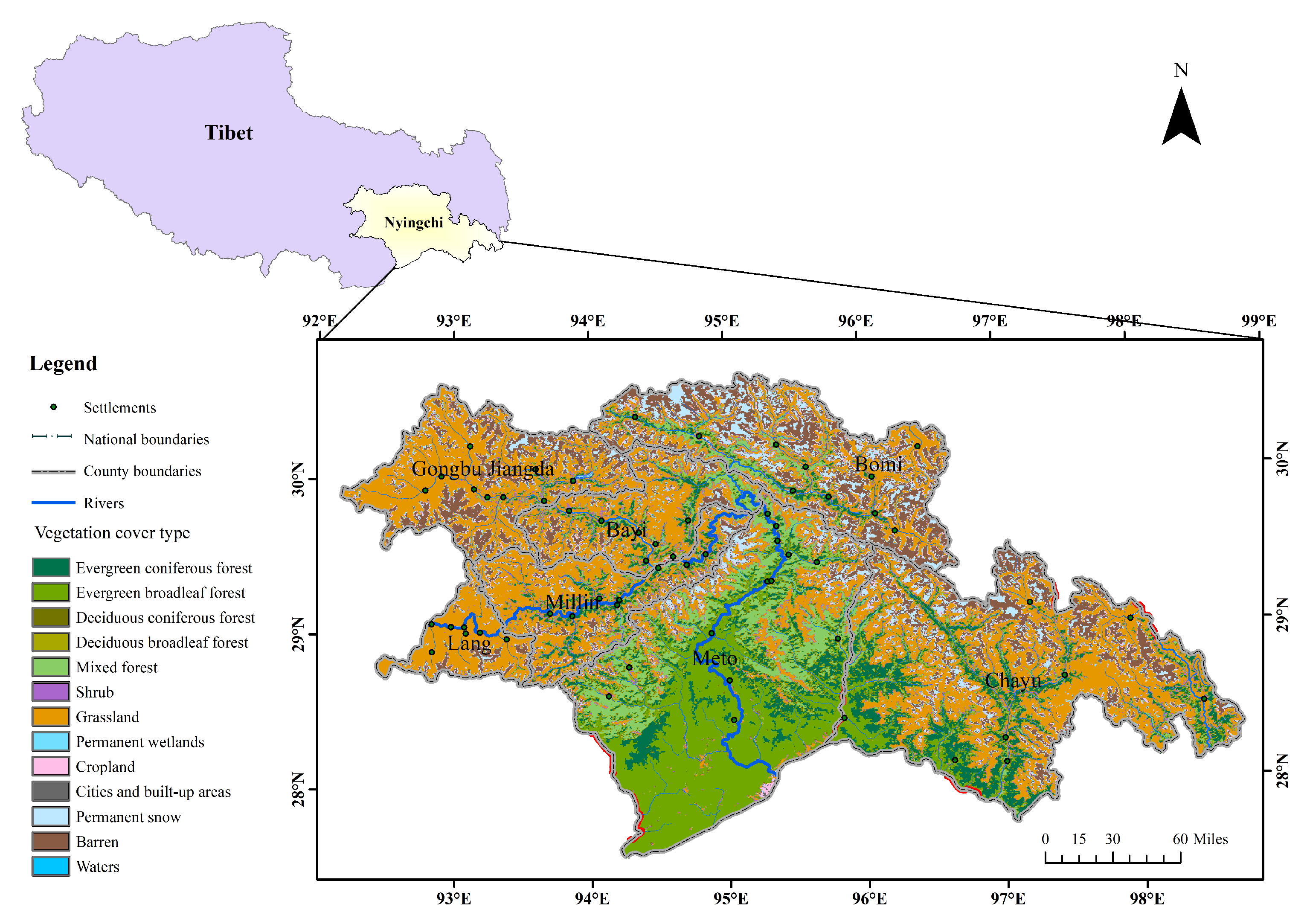
2.1. Study Area

The study area, Nyingchi (Figure 1), is situated in the southeastern part of Tibet Autonomous Region, bordering India and Myanmar, along the middle and lower reaches of the Yarlung Zangbo River. Its altitude ranges from 150 to 7782 m, with the Nyenchen Tanglha Mountains in the north, the Himalayas in the south, the residual ridge of Gangdise Mountains in the northwest, the Hengduan Mountains in the east, and the Yarlung Zangbo Grand Canyon in the center, which is the largest canyon in the world. The relative altitude difference in Nyingchi reaches up to 7627 m, and the terrain slopes from northwest to southeast with significant undulations.

Nyingchi belongs to the oceanic Indian monsoon climate, which provides favorable water and heat conditions. Due to the large altitude difference, the vertical zonation in Nyingchi is obvious, and there is a significant difference in vertical climate zones between the north and south slopes. The southern slope has five climate zones, ranging from the mountain base to the mountain top, while the northern slope is situated in the plateau interior with less water vapor, resulting in a relatively simple vertical climate zone spectrum.

The average temperature in Nyingchi varies from 6 to 17 °C, which is comparatively high in relation to areas at the same latitude, albeit with relatively small annual and diurnal temperature fluctuations. The area is rich in water vapor, and the rainy season begins in June and lasts until September, with abundant precipitation during summer. Precipitation in Nyingchi is mostly irregular and evenly continuous, with the majority of areas receiving annual rainfall between 500 and 1000 mm [24]. However, due to the influence of topography, there are notable differences between regions, such as in the western Yarlung Zangbo River, where annual precipitation is less than 500 mm, while in Motuo County, situated on the southern foothills of the Himalayas, the annual precipitation can exceed 2000 mm.

Nyingchi boasts a dense river network and abundant runoff. The Yarlung Tsangpo River system dominates the northwest part of the region, including many tributaries like Niangqu, Niayang, and Yigong Tsangpo rivers. The central part of the region is home to the main stem of the Yarlung Tsangpo River, along with tributaries such as Danbaqu, Chayu, and others, which flow south and join the Brahmaputra River. The eastern part of the region features several tributaries of the Nu River system located in the Hengduan Mountains.

The land cover types in Nyingchi region are mainly forests and grasslands. Forests are mainly distributed in the valley areas below 3500 m above sea level, with concentrated distribution in the central and southern parts, and branching distribution in other areas according to topography. Shrubs and grasslands are mainly distributed in the plateau areas at altitudes of 3500–5000 m, with grasslands distributed in large areas and shrubs distributed in small scattered areas. In addition, the mountaintop areas in the central and northern parts with altitudes greater than 5000 m are covered with large permanent snowfields, which are the source of many rivers. In general, from the foothills to the mountain tops, the land cover and vegetation types in Nyingchi region are evergreen broadleaved forests, evergreen coniferous forests, mixed coniferous and broadleaved forests, shrublands, grasslands, and permanent snowfields.

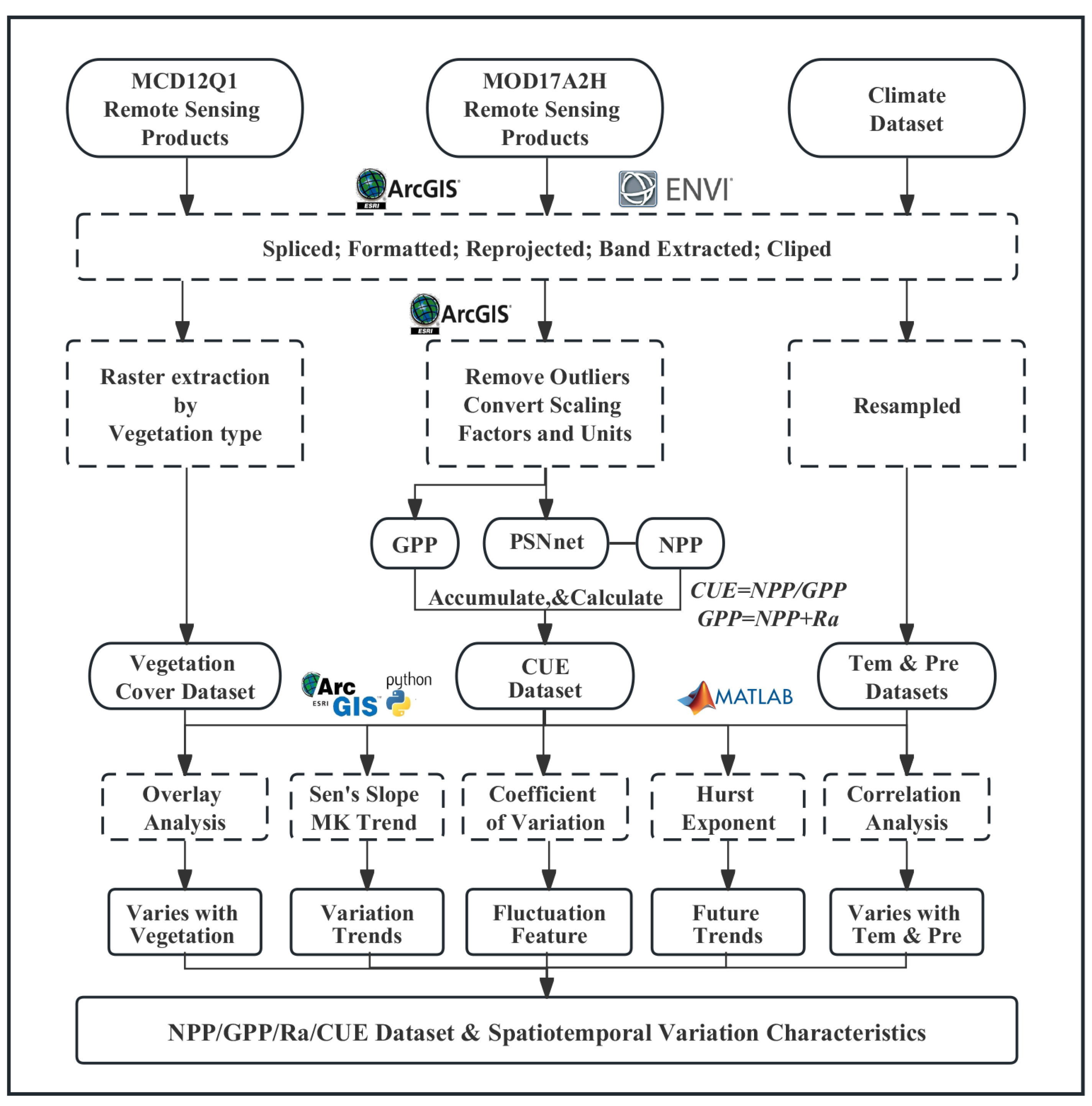
2.2. Data

2.2.1. MODIS GPP, NPP Dataset and Calculation of CUE

The land net primary productivity (NPP) and gross primary productivity (GPP) data used in this study are sourced from the MOD17A2HGF Version 6 remote sensing product in the Moderate-resolution Imaging Spectroradiometer (MODIS) series, which was downloaded from the NASA website (http://modis.gsfc.nasa.gov/, accessed on 12 August 2022). This product provides continuous global monitoring of gross primary productivity data (GPP) and net photosynthesis data (${\mathrm{PSN}}_{net}$), with a temporal resolution of 8 days and a spatial resolution of 500 m. Based on the quality control (QC) labels of each pixel, MOD17A2HGF removes poor-quality inputs from the 8-day leaf area index and photosynthetically active radiation fraction (FPAR/LAI) in MOD17, and then supplements its values through linear interpolation. The data has also undergone radiometric, atmospheric, and geometric corrections. Using ArcGIS 10.2 software, the MOD17A2HGF data from 2001 to 2022 were formatted, joined, clipped, processed to remove outliers as indicated in the metadata file, convert scaling factors, and units, in order to obtain the raw values of GPP and ${\mathrm{PSN}}_{net}$.

GPP is the total amount of carbon fixed by plants in an ecosystem, while NPP is the amount of carbon remaining after plant respiration. $R_a$ (autotrophic respiration) is the amount of carbon lost due to plant respiration. $R_a$ can be divided into maintenance respiration ($R_m$) and growth respiration ($R_g$), and their relationship can be expressed as:

$$NPP=GPP-R_a=GPP-R_m-R_g$$

(1)

${\mathrm{PSN}}_{net}$ is the amount of carbon fixed by plants through photosynthesis, minus the amount of carbon lost through plant maintenance respiration ($R_m$) [25]. Therefore, ${\mathrm{PSN}}_{net}$ can be used to calculate NPP by subtracting the amount of carbon lost through growth respiration ($R_g$). Based on the algorithm of MOD17A2, the value of growth respiration ($R_g$) is estimated to be 25% of NPP using empirical parameterization [26]. Therefore, NPP can be directly calculated using ${\mathrm{PSN}}_{net}$:

$${\mathrm{PSN}}_{net}=GPP-R_m$$

(2)

$$R_g=0.25\ast NPP$$

(3)

$$NPP=0.8\ast PS{N}_{net}$$

(4)

The 8-day NPP and GPP data obtained in this study were aggregated into monthly and yearly data for the 22-year period based on their coverage dates. Next, the vegetation carbon use efficiency (CUE) value was calculated for each pixel using the definition formula of CUE:

$$CUE=\frac{NPP}{GPP}$$

(5)

where CUE represents the vegetation carbon use efficiency of the ecosystem; $NPP$ is the net primary productivity of vegetation ($\mathrm{gc}{\mathrm{m}}^{-2}·{\mathrm{t}}^{-1}$); $GPP$ is the gross primary productivity of vegetation ($\mathrm{gc}{\mathrm{m}}^{-2}·{\mathrm{t}}^{-1}$). The total $NPP$, $GPP$ and annual CUE distribution in 2022 are shown in Figure A1, Figure A2 and Figure A3.

2.2.2. Land Cover Dataset

The land cover data of the Nyingchi area in this study was obtained from the MODIS MCD12Q1 land cover type product, which has a temporal resolution of 1 year and a spatial resolution of 500 m. The MCD12Q1 product provides five land cover classification schemes, which utilize supervised decision tree information extraction technology for land classification [27]. The IGBP global vegetation classification scheme was selected in this study, which includes 17 major land cover types, consisting of 11 natural vegetation types, 3 land development and mosaic land cover types, and 3 non-vegetated land cover types [28]. The MCD12Q1 data were processed by splicing, formatting, reprojection, and band extraction using the ENVI-MCTK plugin (Multi-Class Toolkit) to obtain the TIFF dataset under the IGBP classification scheme. The dataset was clipped using ArcGIS 10.2 software to obtain the land cover data of the Nyingchi area for each year. Subsequent overlay analysis was performed according to vegetation categories to obtain NPP/GPP/Ra/CUE data for each vegetation type.

2.2.3. Climate Dataset

The monthly precipitation (Pre) and mean temperature (Tem) data from 2001 to 2021 in Nyingchi area were obtained from the National Earth System Science Data Center, National Science & Technology Infrastructure of China (http://www.geodata.cn, accessed on 14 August 2022). The temporal resolution and spatial resolution were 1-month and 1 km, respectively. The data were generated by Peng Shouzhang based on the global 0.5° climate dataset released by CRU and the high-resolution climate dataset released by WorldClim, using the Delta spatial downscaling scheme to downscale the monthly precipitation and mean temperature data in China [29]. After obtaining the data, ArcGIS 10.2 software was used for format conversion, reprojection, band separation, and clipping, and finally resampled to obtain the 500 m meteorological dataset in Nyingchi area for 21 years. This dataset was used for testing the correlation between CUE, temperature and precipitation in the subsequent analysis.

2.3. Analytical Methods

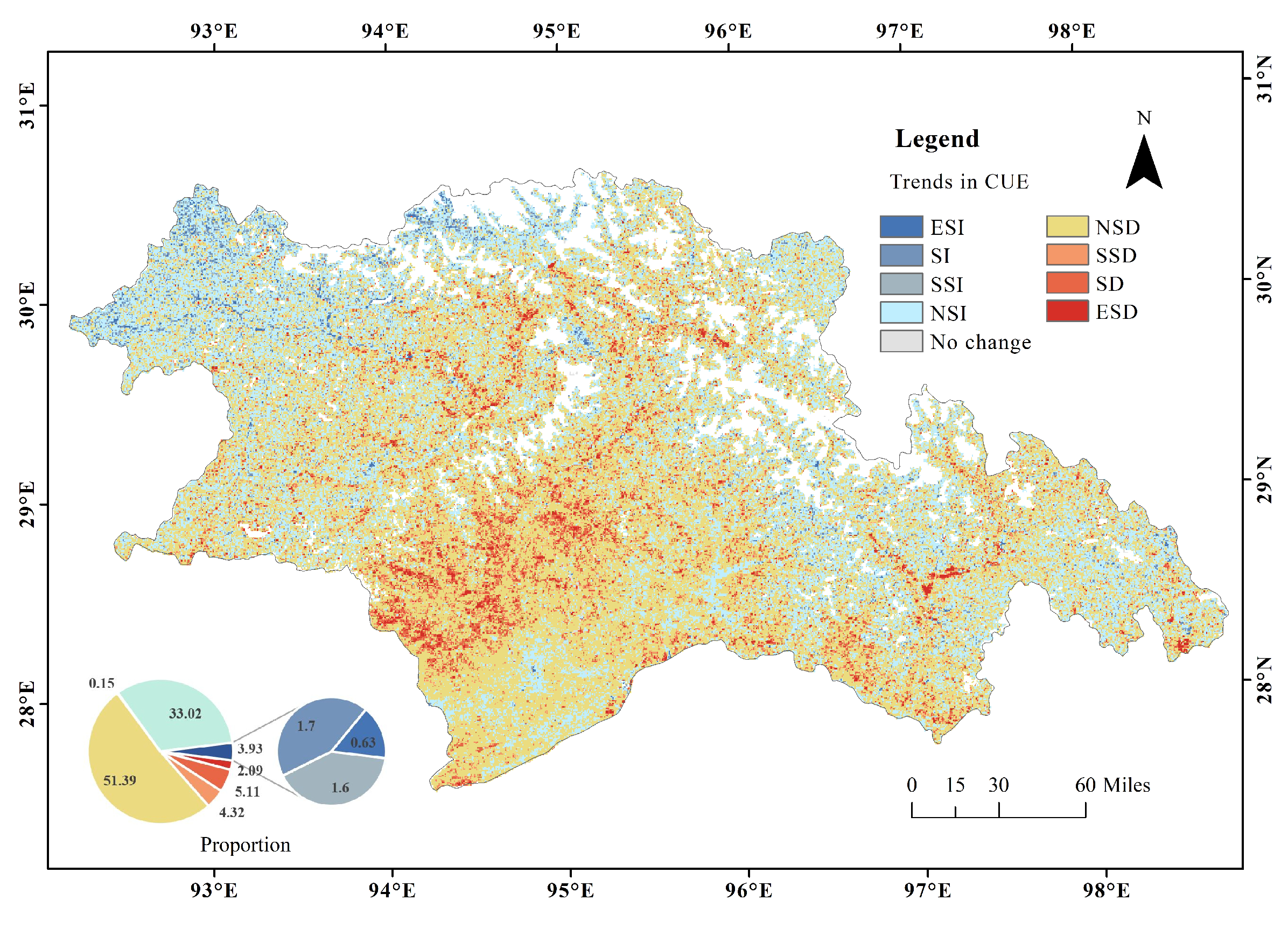
2.3.1. Theil-Sen Median Slope Estimator and Mann-Kendall Trend Analysis

The Theil-Sen median method (also known as Sen’s slope estimation) is a robust non-parametric statistical method for trend analysis that is insensitive to measurement errors and outliers [30]. It is suitable for analyzing trends in long-time series data. The formula for calculating the trend value $\beta$ of CUE is:

$$\beta =Median\left(\frac{{CUE}_j-{CUE}_i}{j-i}\right)\forall j>i$$

(6)

where $Median\left(\right)$ represents the calculation of the median. If $\beta$ is greater than zero, it indicates an increasing trend of vegetation CUE, and vice versa for a decreasing trend.

The Mann-Kendall test is a non-parametric method for testing time series trends. It does not require the measured values to follow a normal distribution and is not affected by missing or outlier values, making it suitable for testing significant trends in long time series data. The process is as follows: at the pixel scale, for a sequence of ${CUE}_1,{CUE}_2,\dots ,{CUE}_n$, all pairwise values (${CUE}_i,{CUE}_j,j>i$) are first used to determine the size relationship (S) between ${CUE}_i$ and ${CUE}_j$.

The hypothesis is as follows: $H_0$: The values of CUE in the sequence are randomly arranged, that is, there is no significant trend; $H_1$: The CUE sequence shows an upward or downward trend. The calculation formula for the test statistic S is:

$$S=\sum _{i=1}^{n-1}\sum _{j=i+1}^{n}sgn({CUE}_j-{CUE}_i)$$

(7)

where $sgn\left(\right)$ is a symbolic function, and the calculation formula is:

$$sgn({CUE}_j-{CUE}_i)=\left\{\begin{array}{cc}+1& {CUE}_j-{CUE}_i>0\\ 0& {CUE}_j-{CUE}_i=0\\ -1& {CUE}_j-{CUE}_i<0\end{array}\right.$$

(8)

The trend test is performed using the test statistic Z, which is calculated as follows:

$$Z=\left\{\begin{array}{cc}\frac{S}{\sqrt{Var\left(S\right)}}& (S>0)\\ 0& (S=0)\\ \frac{S+1}{\sqrt{Var\left(S\right)}}& (S<0)\end{array}\right.$$

(9)

The formula for calculating $Var$ is:

$$Var\left(S\right)=\frac{n(n-1)(2n+5)}{18}$$

(10)

where n is the number of data in the sequence, m is the number of groups with repeated data in the sequence, and $t_i$ is the number of repeated data in the i-th group of repeated data.

The double-sided trend test is used to obtain the critical value $Z_{1-\alpha /2}$ at a given significance level. When $\left|Z\right|\le Z_{1-\alpha /2}$, the null hypothesis $H_0$ of no significant trend is accepted; if $\left|Z\right|>Z_{1-\alpha /2}$, then $H_0$ is rejected and a significant trend is considered. In this paper, the significance level is set at $\alpha =0.05$, so the critical value is $Z_{1-\alpha /2}=\pm 1.96$. When the absolute value of Z is greater than 1.65, 1.96, and 2.58, the trend passes the significance test with confidence levels of 90%, 95%, and 99%. The significance of the trend feature increases in order [31].

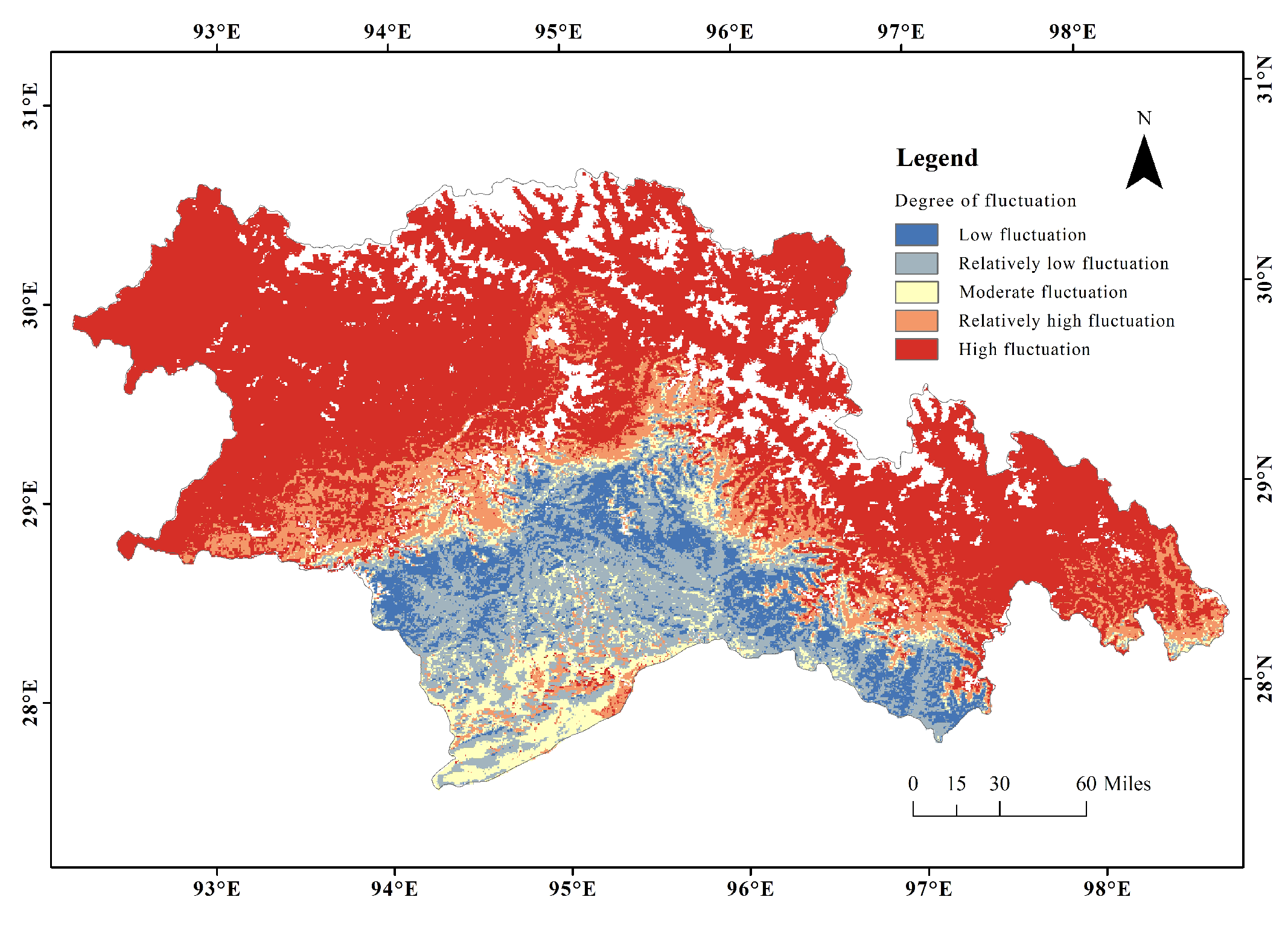
2.3.2. Spatiotemporal Stability Analysis

In this study, the coefficient of variation ($CV$) was used to reflect the degree of variation of vegetation CUE in the time series. The $CV$ is the ratio of the standard deviation of the data to its mean, which can well reflect the degree of variation of the data in the time series, and evaluate the temporal stability of the data [32,33]. The calculation formula is:

$$CV=\frac{1}{\overline{CUE}}\sqrt{\frac{{\sum }_{i=1}^n{({CUE}_i-\overline{CUE})}^2}{n-1}}$$

(11)

where $CV$ represents the coefficient of variation of the pixel, ${CUE}_i$ is the CUE of the i-th time period, and $\overline{CUE}$ is the average value of CUE in the study sequence. When the $CV$ value is larger, it indicates that the data is more dispersed and the vegetation CUE varies greatly; when the $CV$ value is smaller, it indicates that the data is more compact and the degree of CUE variation is small. Following the grading method of $CV$ in [33], the regional $CV$ is divided into five levels: $CV<0.05$ for low fluctuation, $0.05\le CV<0.10$ for relatively low fluctuation $0.10\le CV<0.15$ for medium fluctuation, $0.15\le CV<0.20$ for relatively high fluctuation, and $CV\ge 0.20$ for high fluctuation.

2.3.3. Correlation Analysis

Due to the complex relationship between research variables, the simple Pearson correlation coefficient can only reflect the surface properties of the correlation between two variables, but cannot truly reflect the degree of linear correlation between variables. Therefore, based on a long sequence dataset, this paper calculates the partial correlation coefficient at the pixel scale to reflect the correlation between two variables [34]. The formula for calculating the first-order partial correlation coefficient is:

$$r_{xy·z}=\frac{r_{xy}-r_{xz}·r_{yz}}{\sqrt{(1-{r_{xz}}^2)(1-{r_{yz}}^2)}}$$

(12)

where $r_{xy·z}$ represents the partial correlation coefficient between variables X and Y in a certain pixel when controlling for variable Z, $r_{xy}$, $r_{xz}$, $r_{xz}$ are the simple correlation coefficients between variables X, Y, and Z.

Hypothesis testing is conducted on the partial correlation coefficient to reflect the significance level of the correlation between two variables. The null hypothesis of the partial correlation coefficient test is that the partial correlation coefficient between the two variables in the population is zero. The t-test method is used to test this hypothesis, and the calculation formula is as follows:

$$t=\frac{\sqrt{n-k-2}·r}{\sqrt{1-r^2}}$$

(13)

where r is the partial correlation coefficient between the two variables, n is the number of sample observations, k is the number of control variables, and $n-k-2$ is the degree of freedom. When $t>t_{0.05}(n-k-2)$, i.e., the significance level $p<0.05$, the null hypothesis is rejected, and it is considered that there is a significant correlation between the two variables. In particular, when $p<0.01$, it is considered that there is an extremely significant correlation between the two variables.

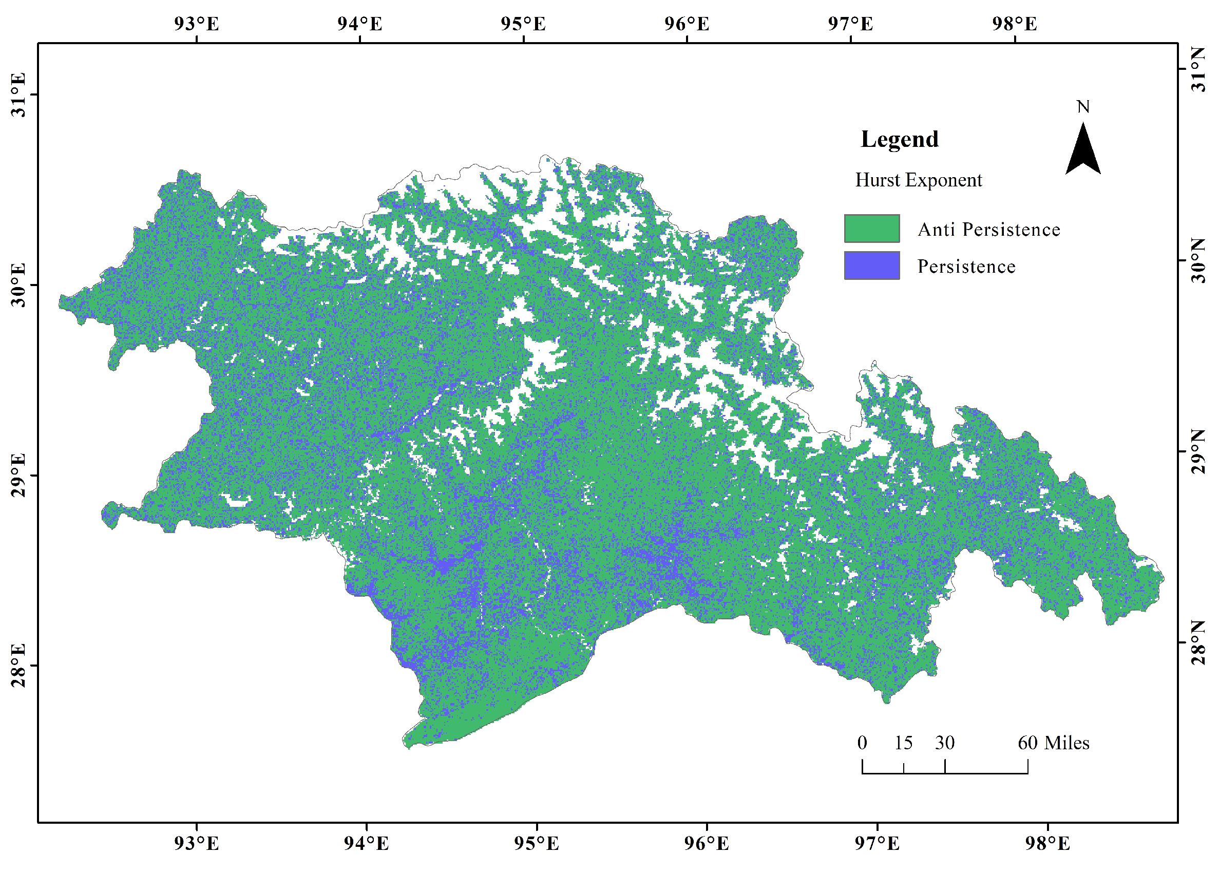
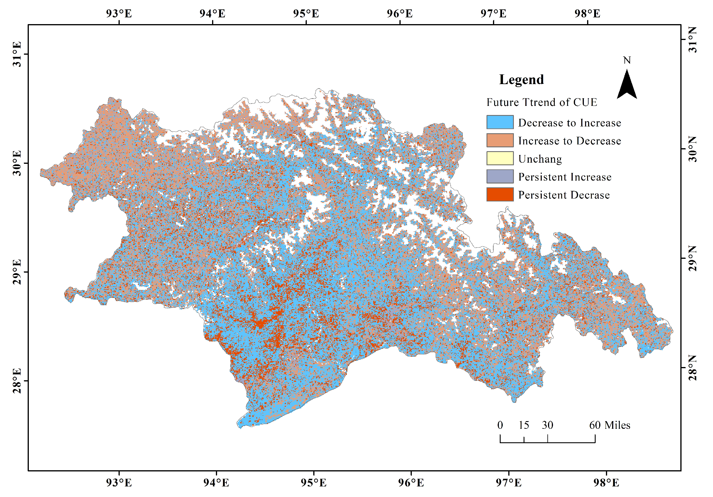
2.3.4. Future Trend Analysis

In geography, the Hurst exponent is an effective method for describing spatial self-similarity and long-term dependence phenomena [35]. In this paper, the Hurst exponent is used to reflect the short-term trend of vegetation CUE in the future by the rescaled range (R/S) analysis method proposed by Harold Edwin Hurst, a British hydrologist [36,37]. The calculation method is as follows: for the vegetation CUE data sequence from 2001 to 2022: $\left\{CUE\left(i\right)\right\},i=1,2\dots n$, at the pixel scale, for any positive integer $\tau$, define the parameter of the time series as follows:

Differential sequence:

$$△CU{E}_i=CU{E}_i-CU{E}_{i-1}$$

(14)

Mean sequence:

$$\overline{\Delta CU{E}_{\left(\tau \right)}}=\frac{1}{\tau }\sum _{i=1}^{\tau }\Delta CU{E}_i(\tau =1,2\dots n)$$

(15)

Cumulative deviation sequence:

$$X_{(t,\tau )}=\sum _{i=1}^{\tau }\left(\Delta CU{E}_i-\overline{\Delta CU{E}_{\left(\tau \right)}}\right)(1\le t\le \tau )$$

(16)

Range sequence:

$$R_{\left(\tau \right)}=\underset{1\le t\le \tau }{max}{X}_{(t,\tau )}-\underset{1\le t\le \tau }{min}{X}_{(t,\tau )}(\tau =1,2,\dots n)$$

(17)

Standard deviation sequence:

$$S_{\left(\tau \right)}={\left[\frac{1}{\tau }\sum _{i=1}^{\tau }{\left(\Delta CU{E}_i-\overline{\Delta CU{E}_{\left(\tau \right)}}\right)}^2\right]}^{1/2}(\tau =1,2,\dots n)$$

(18)

For the ratio $\frac{R\left(\tau \right)}{S\left(\tau \right)}\cong \frac{R}{S}$, if there exists $\frac{R}{S}\propto {\tau }^H$, it indicates the presence of Hurst phenomenon in the analyzed time series, where H is the Hurst exponent. The value of H is calculated by using the least squares method to fit a line with the slope on the double logarithmic coordinates ($lni$,$ln\frac{R}{S}$). The classification is based on the value of H, where $0.5<H<1$ indicates a persistent sequence of regional CUE, meaning that the future trend is the same as the current trend; $H=0.5$ indicates a random sequence of regional CUE with no long-term persistence characteristic; and $0<H<0.5$ indicates an anti-persistent sequence of regional CUE, meaning that the future trend is opposite to the current trend [38].

Overall, the data processing and analysis flow of this article is shown in Figure 2.

3. Results

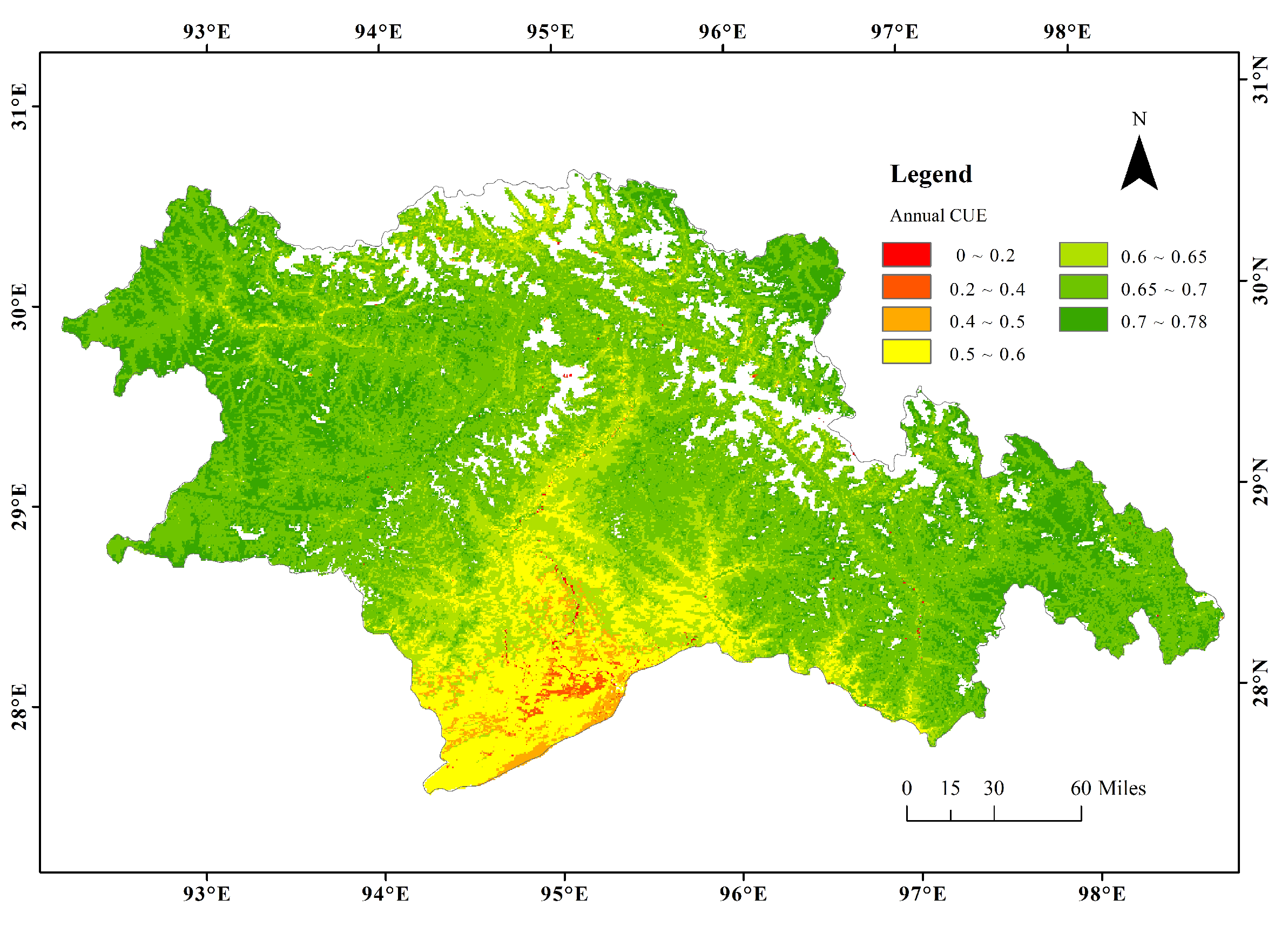
3.1. Spatial Patterns of CUE

The average distribution of annual CUE in the Nyingchi area is illustrated in Figure 3. The white regions in the figure represent areas without vegetation, such as water bodies and perennial snow, and therefore have no NPP or GPP values [26]. The annual average CUE in the Nyingchi ranges from 0 to 0.78, with an average of 0.66. More than 99% of the area fluctuates between 0.2 and 0.8, consistent with previous studies [39,40,41], suggesting the validity of the data.

The analysis indicates that the overall pattern of CUE in Nyingchi is a gradual decrease from both sides to the center and from south to north. This distribution pattern is related to the elevation and vegetation cover types of the region. The area with an annual CUE in the range of 0–0.4 accounts for 4.8% of the total area, primarily located in the evergreen broadleaved forest in the south, with scattered distribution in the Yarlung Zangbo River valley. The area with an annual CUE in the range of 0.4–0.5 accounts for 1.47% and is mainly found in the broadleaved forest, shrubs, sparse forest, and residential areas below 2000 m in the southern river valley. The area with an annual CUE in the range of 0.5–0.6 accounts for 9.77% and is mainly concentrated in the evergreen broadleaved forest around 1500 m in the south. The area with an annual CUE in the range of 0.6–0.65 accounts for 15.16% and is mainly distributed in the needle-leaf and broad-leaved mixed forest between 2000–3000 m in the south, and sporadically distributed in the central river valley area, following the shape of the river network.

Most of the Nyingchi area has an annual CUE between 0.65–0.7, accounting for 53.18% of the total area, primarily concentrated in the grassland at 4000–5500 m and the coniferous forest between 2000–3000 m. The area with a CUE between 0.7–0.78 is a high-value area, accounting for 19.95% of Nyingchi, primarily distributed in the boundary areas above 5000 m, including mixed grassland, farmland, and barren land (with a vegetation coverage rate of less than 10% year-round).

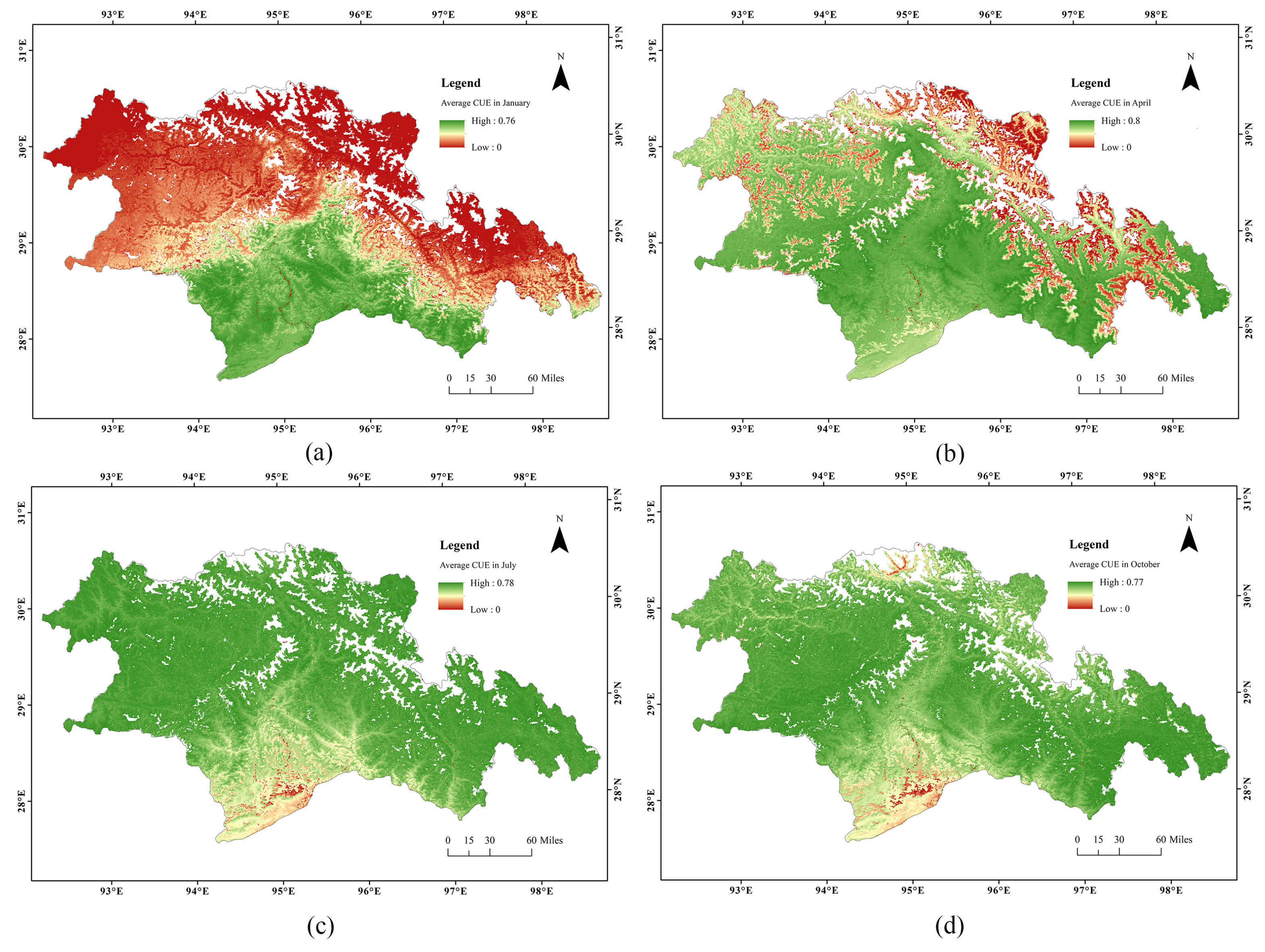
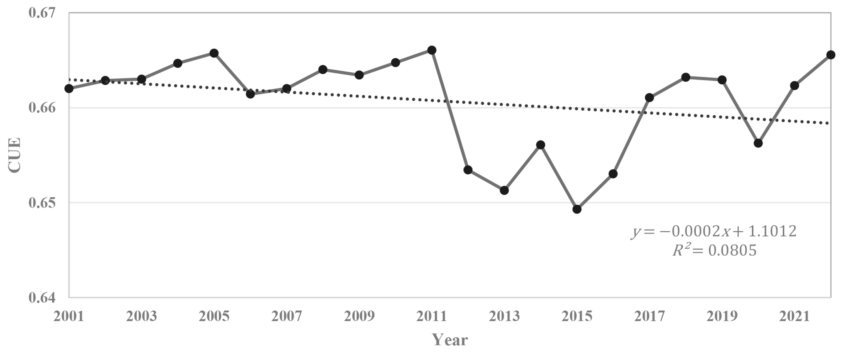
3.2. Intra-Annual and Inter-Annual Variation of CUE

The cyclical pattern of vegetation CUE throughout the year in the Nyingchi area is illustrated in Figure 4. From December to February (Figure 4a), the CUE is generally low, as indicated by the south-to-north boundary near 29°N, where the CUE in the northern region is mostly below 0.3, while the CUE in the southern region maintains a level of 0.65. In the growing season, from March to May (Figure 4a,b), the CUE in grasslands and coniferous forest areas in the north rapidly increases from south to north, climbing to a level of 0.5, while the CUE in the southern forest area decreases by about 0.1 compared to winter. From spring to summer (Figure 4b,c), the CUE in areas with low vegetation coverage quickly rises to above 0.65, while the CUE in shrubs, coniferous forest, and mixed forest areas rises to above 0.6, and the CUE in evergreen broadleaf forest areas continues to decline to 0.5 or below. In particular, the forest area at the southern boundary drops to below 0.3, which is the lowest value in the region during this period. From June to September, most areas in Nyingchi reach and stabilize in the high CUE area, with an average CUE of 0.66 or higher, except for the southern evergreen broadleaf forest area. After October (Figure 4d), as the temperature drops, the CUE in shrubland, grassland, and uncultivated land gradually declines to the level of winter (below 0.3), starting from the northern boundary area, while the CUE in the southern forest area begins to rise and eventually stabilizes at 0.65.

As outlined in Section 2.3.2, the coefficient of variation (CV) was utilized to measure the magnitude of variation and stability in vegetation changes throughout the growth cycle. The resultant CV values were categorized into five levels [33]. Figure 5 demonstrates that the Nyingchi area is demarcated by a central line in the vicinity of 29°N, with the northern region characterized by a high degree of fluctuation in CUE throughout the year. The transitional zone between grassland and forest in the central region exhibits a relatively high degree of fluctuation. Conversely, the CUE of the evergreen broad-leaved forest above 1000 m in the southern region demonstrates moderate and relatively low fluctuation. With increasing altitude and latitude, the vegetation type changes from broad-leaved forests to coniferous forests, and the stability of CUE consequently increases. The region with the highest degree of CUE stability is the evergreen coniferous and mixed forest area situated between an altitude of 2000–4000 m and a latitude of 28°N to 29°N. CUE has remained in a low-fluctuation state in this region for an extended period.

The annual inter-annual variation of the average CUE in Nyingchi region over 22 years is shown in Figure 6. The inter-annual CUE has been maintained at a level of around 0.66, and the trend line fitted by a simple linear regression shows a slight downward trend in annual CUE overall, but it is not significant. The highest annual mean CUE value occurred in 2011, at 0.666, and the lowest occurred in 2015, at 0.649. The CUE level in Nyingchi was relatively stable between 2001 and 2011, with only slight fluctuations within a range of no more than 0.005. However, after 2011, the amplitude of CUE fluctuations increased significantly, with a fluctuation range exceeding 0.01. From 2011 to 2013, there was a rapid decline in CUE, while from 2015 to 2017, there was a significant increase, recovering to a level of 0.661 in 2017. Overall, the stability of CUE during the latter 11 years was lower than that of the previous 11 years.

After conducting an overlay analysis with the vegetation status of the underlying surface, a line graph of the annual CUE changes for each vegetation type from 2001 to 2022 was obtained and is presented in Figure 7. The analysis revealed that the range and fluctuation of CUE differ among different vegetation types on an annual scale. The evergreen broad-leaved forests have an average CUE value ranging from 0.55 to 0.6, with the most significant fluctuation observed. In contrast, the CUE values of shrubs, mixed forests, deciduous broadleaved forests, evergreen coniferous forests, and deciduous coniferous forests are concentrated around 0.64 to 0.67, and the fluctuation range and overall trend of these categories are roughly similar, with relatively stable CUE levels. The barren, urban, farmland, and grassland have CUE average values ranging from 0.68 to 0.7, which are high CUE value areas in Nyingchi. Barren land (vegetation coverage less than 10%) has the highest CUE level. The annual CUE fluctuations of these four types of land cover are weak, and the annual averages remain relatively constant.

3.3. The Variation Trend of CUE

Estimation of Sen’s slope and MK trend analysis were performed on the continuous multi-year CUE dataset, and the results of both analyses were combined to classify the trend change characteristics into 9 categories [42,43]. The distribution and area proportion of each trend change category are depicted in Figure 8. The results show that in 62.91% of Nyingchi, the CUE exhibited a decreasing trend, and 51.39% showed no significant decrease, with the highest percentage being observed in the broadleaved forest, coniferous forest, mixed forest areas, and the transitional zone between forest and grassland in the central part of Nyingchi. The proportion of areas with significant and extremely significant CUE decrease was 7.2%, mainly distributed in the coniferous forest and mixed forest areas near the Himalayas in the southwest of Nyingchi, as well as the mixed forest area in the valley zone of the central and eastern regions. In 36.95% of the area of Nyingchi, the CUE showed an increasing trend, and 33.02% showed significant increasing trend, mainly distributed in the grassland in the north of Gyangze, the middle part of Chayu county in the north of Bomê county, and the broadleaved forest in the south of Motuo. The areas with significant or extremely significant CUE increase were 2.33%, mainly distributed in the grassland and barren at the foothills of the Gangdise Mountains in Nyingchi and the forest-grassland mixed area in the upper reaches of the Yigong and Neyang rivers.

Using the Hurst exponent method, this study aimed to detect the long-term persistence trend of CUE in the Nyingchi region, as depicted in Figure 9. Results indicate that 75.95% of the region in Nyingchi exhibits the “anti-persistence” trend, which implies that the future trend will be opposite to the current trend. Meanwhile, 24.05% of the region shows the “persistence” trend, which suggests that the future trend will be the same as the current trend. Specifically, the persistence trend mainly occurs in grasslands located in the northwest and southeast regions, near the Himalayas in the southwest, and in forests near Dalan River in the southeast, while the rest are scattered throughout the region.

The future trend of CUE in Nyingchi was determined by overlaying the long-term trends obtained from Hurst exponent analysis with Sen’s slope estimation and MK trend analysis results [25], and the results are presented in Figure 10. The analysis revealed that 47.82% of the CUE areas in Nyingchi will experience a trend reversal from decreasing to increasing, which is mainly concentrated in the forest and forest-grass mixed zones on both sides of the river valleys in the central part of Nyingchi. Furthermore, 28.10% of the CUE areas will exhibit a trend reversal from increasing to decreasing, mainly distributed in the grasslands in the northwest and central-eastern parts of the region. The areas with continuous CUE increase account for 8.89% and are sparsely distributed in the grassland in the west and the evergreen broad-leaved forest in the south. The areas with continuous CUE decrease account for 15.15%, mainly distributed on both sides of the Yarlung Zangbo River in the central region, the Himalayan region near the southwestern border, and the Dalan River area in the southeast.

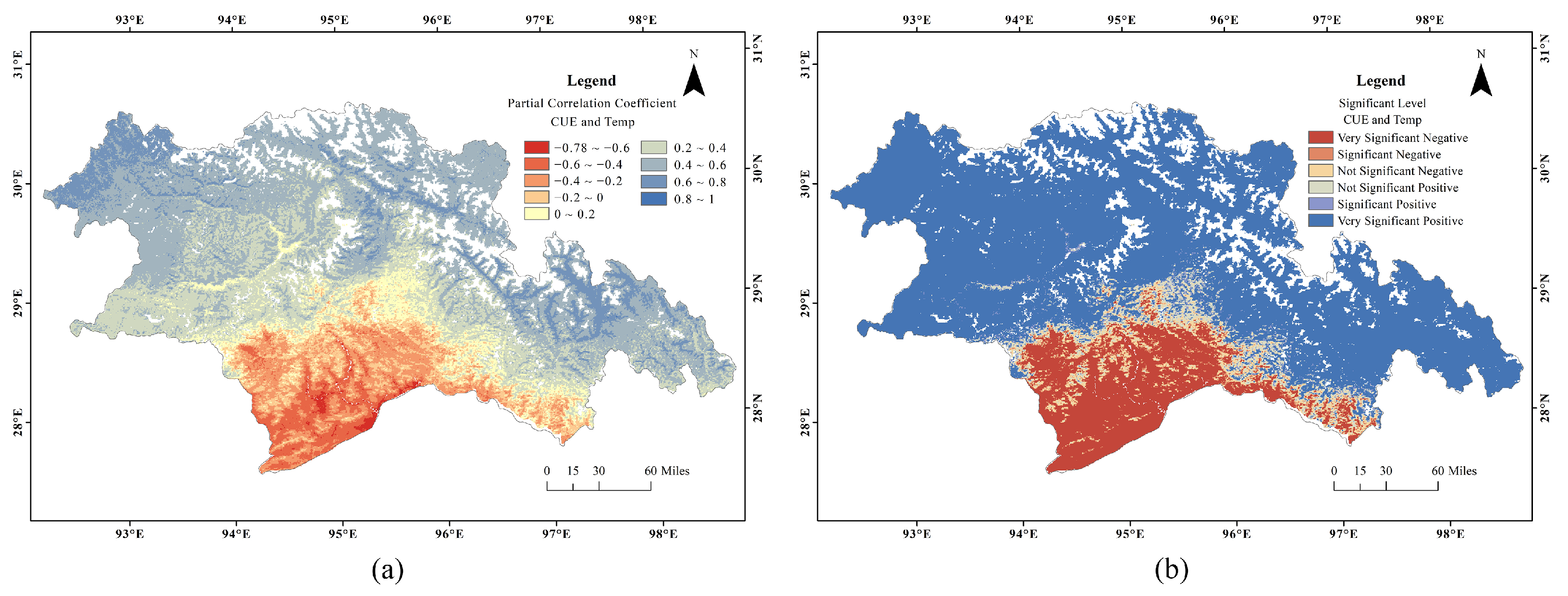
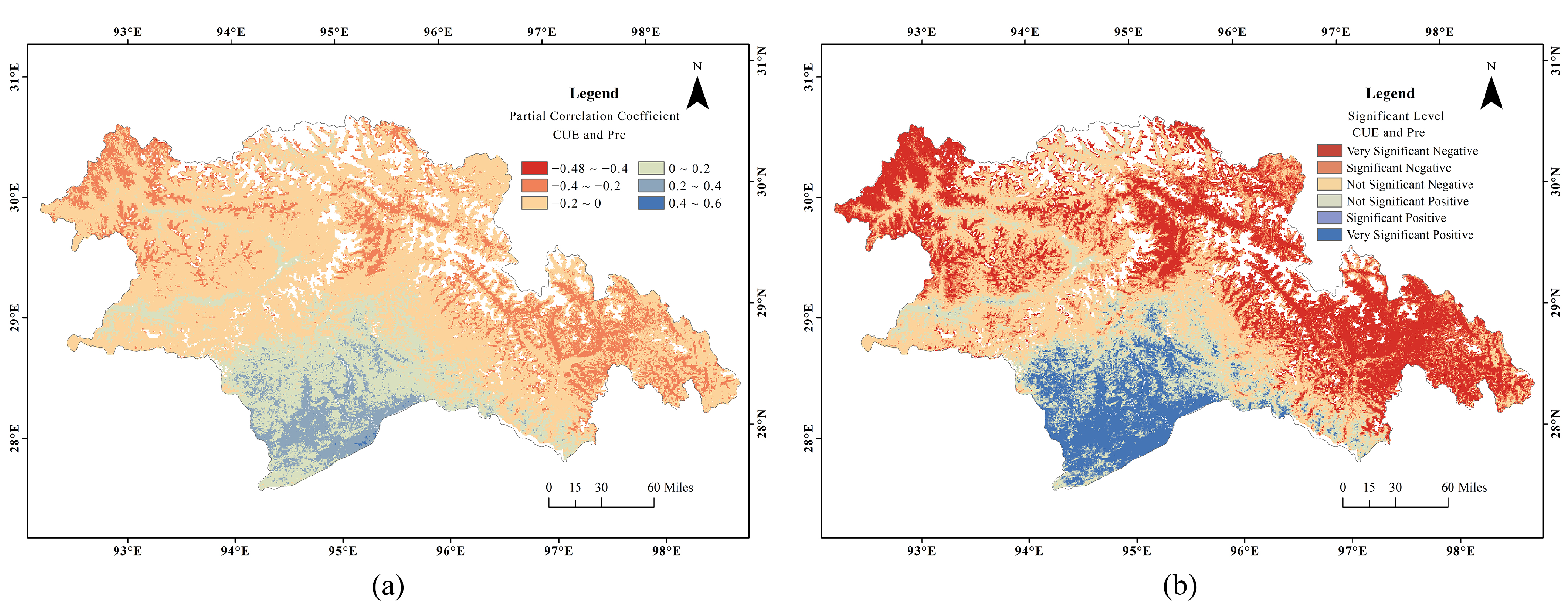
3.4. Variation of CUE with Temperature and Precipitation

Combining partial correlation coefficients and significance test formulas, this paper calculates the correlation between CUE and temperature/precipitation at the pixel scale based on the monthly datasets from 2001 to 2021, aiming to explore the relationship between CUE variation and temperature/precipitation [44]. Investigating the correlation at the pixel scale can better control unrelated variables and reduce the noise generated by extreme or abrupt temperature, precipitation, and CUE values.

After removing the effect of the precipitation factor, the partial correlation coefficient between CUE and temperature in the Nyingchi region was calculated and subjected to significance testing. The results, as presented in Figure 11, showed that the partial correlation coefficient ranged from −0.79 to 1. Positive correlations accounted for 79.9% of the total area, while negative correlations accounted for 20.1%. Specifically, areas with a strong positive correlation (r > 0.6) were mainly distributed in the upstream grasslands of the Niangqu River, the confluence of rivers at the horseshoe bend of the Yarlung Zangbo River in the central region, and the forests and grasslands in the upstream of Chayu River in the east. Areas showing a strong negative correlation (r < $-0.6$) were mainly found in the shrubs and grasslands in the Yarlung Zangbo River valley south of 28.5°N in Motuo, and in the urban and farmland areas bordering India. In the Nyingchi region, the significance analysis results revealed that 88.88% of the areas showed an extremely significant correlation (p < 0.01) between CUE and temperature, and only 7.89% of the areas showed a non-significant correlation (p > 0.05), mainly in the transition zone of the coefficient variation range between 28°N and 29°N with low correlation (|r| < 0.2). In general, the correlation and significance levels between CUE and temperature in the Nyingchi region decreased from the north and south boundaries towards the central part, with higher correlation levels observed in the canyon and river valley areas.

Similarly, Figure 12 displays the partial correlation coefficient and its significance between CUE and precipitation in Nyingchi region. The results indicate that the correlation between CUE and precipitation in this area is generally weak, with the range of partial correlation coefficients between −0.48 and 0.5. In the total area, the regions with a positive correlation between CUE and precipitation account for 24.42%, mainly located south of the 28.5°N latitude line, with a small proportion in the grasslands of the Yarlung Zangbo River Valley north of the Himalayas. Regions with relatively high correlation (r > 0.3) are mainly found in urban and cropland areas near the southern border. On the other hand, the regions where CUE and precipitation show a negative correlation account for 75.58% of the total area, mainly distributed in areas north of the 28.5°N latitude line. Regions with relatively high negative correlation (r < −0.3) are mainly found in the grasslands of the Gangdise residual range and the upper reaches of the Chayu River. Furthermore, by analyzing the significance level, it was found that the mixed forests, grasslands, and barrens in the northwest and east of Nyingchi, as well as the evergreen forests in the south, show a moderate (|r| > 0.2) and extremely significant correlation between CUE and precipitation, which account for 21.83% of the total area, while the correlation between CUE and precipitation in other areas is relatively low.

Based on the above research, it can be concluded that in the Nyingchi region, the variation patterns of CUE with temperature and precipitation are significantly different in the areas on both sides of the transitional zone between 28°N and 29°N, and the changes in CUE are more closely related to temperature. The global-scale study by Piao et al. [45]. revealed a parabolic relationship between the annual average CUE of forest vegetation and the annual average temperature. This study scaled down the time frame to the monthly scale and obtained consistent results. CUE in the northern part of Nyingchi increases with rising temperatures, while the opposite is observed in the southern part, and areas with an annual average temperature above 12 °C or below 0 °C, CUE is more sensitive to temperature changes. Compared with temperature, the correlation between CUE and precipitation in Nyingchi is relatively weak. Zhang et al.’s global-scale study on CUE [46] demonstrated that CUE decreases with increasing precipitation when the annual precipitation is below 2300 mm, and this conclusion is confirmed in the northern part of Nyingchi (annual precipitation greater than 700 mm). However, in the southern part of Nyingchi, where the annual precipitation is between 300 and 700 mm, an increase in precipitation leads to an increase in NPP and CUE, indicating that CUE in the southern part of Nyingchi may be affected by regional precipitation stress [47,48,49,50].

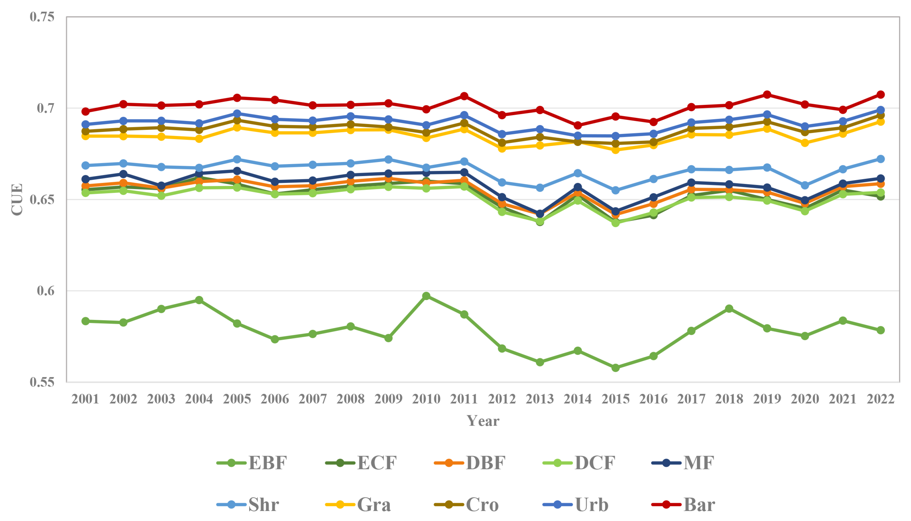
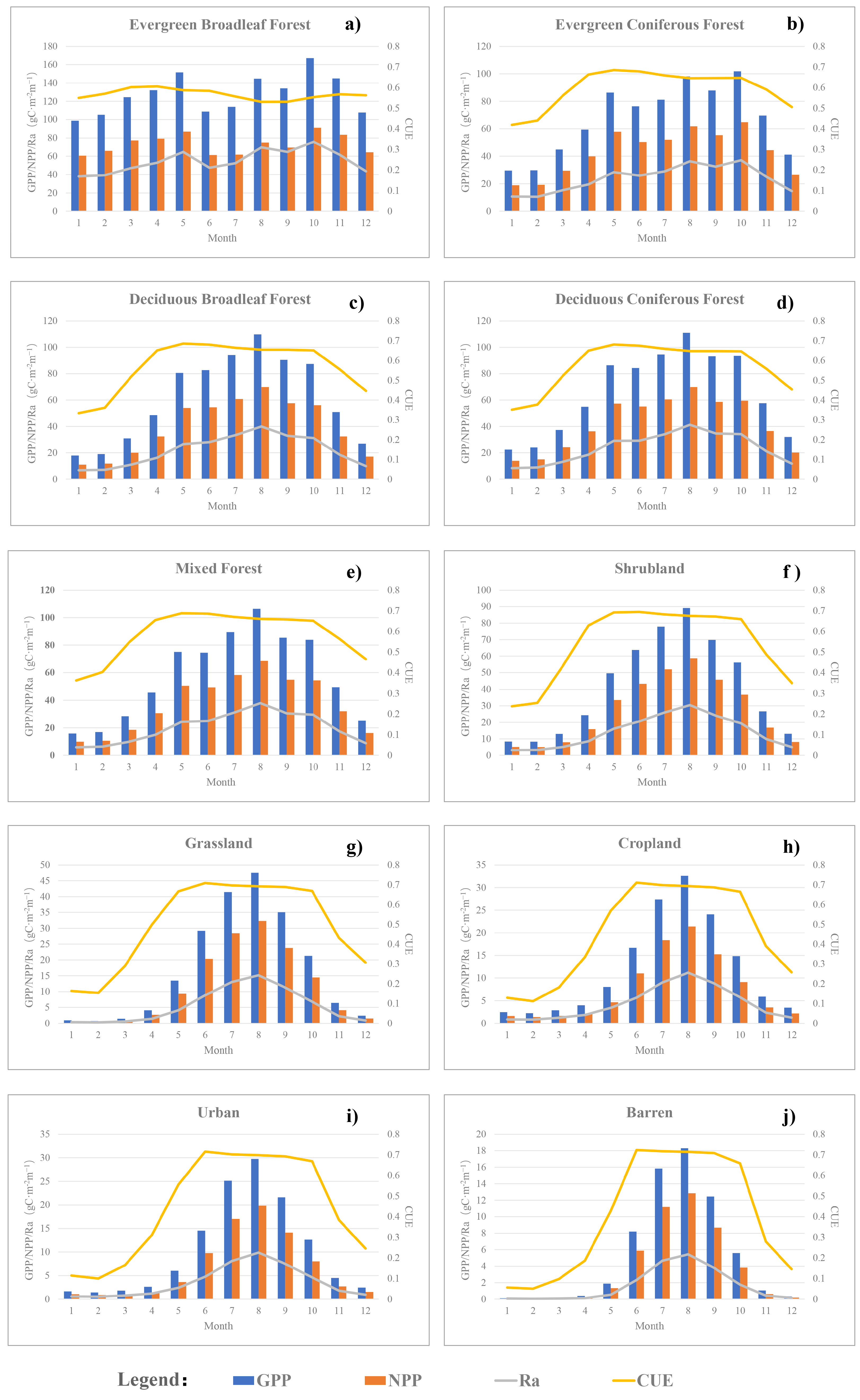
3.5. Cue Changes of Each Vegetation Type in Response to the Growth Process

The average data of NPP/GPP/Ra/CUE for various typical vegetation cover types in Nyingchi region during the growing season are shown in Figure 13. The carbon fixation process of evergreen broadleaved forest vegetation (Figure 13a) is unique due to the combined effects of latitude and topography. This vegetation type exhibits high values in spring and autumn and low values in winter and summer with small fluctuations. This suggests that the ratio of carbon consumption to production is relatively stable during the growth cycle. Although evergreen broadleaved forests have the highest NPP/GPP levels, they also release the most carbon due to respiration. Notably, the high and low periods of NPP, GPP, and CUE do not coincide, and there is a significant productivity trough in June and July during the peak summer period.

Evergreen needleleaf forest is the second vegetation type after evergreen broadleaf forest to have the smallest range of variation in CUE across the growing season. CUE fluctuates between 0.4 and 0.7 throughout the year. Nearly half of the evergreen broadleaf forests in Nyingchi experience winter (December to February) temperatures below 0 °C, resulting in a short dormancy period. As shown in Figure 13b, during this time, the NPP/GPP level of the evergreen needleleaf forest is relatively low, and CUE drops to 0.4–0.5. Similar to the broadleaf forest, there is a slight decrease in productivity in June and July. The peak productivity of evergreen vegetation is in October, and it is speculated that high temperatures during the summer limit the productivity of evergreen vegetation [51].

Deciduous broadleaf forest, deciduous needleleaf forest, and mixed forest (Figure 13c–e) exhibit similar ranges and trends of NPP/GPP/Ra/CUE. These vegetation types have the highest NPP/GPP/Ra levels in summer, followed by spring and autumn, and the lowest in winter. The peak period of CUE is in April-May, when NPP/GPP levels increase rapidly. Therefore, it is inferred that these three types of vegetation perform carbon sequestration at a higher level in the early growing season to meet their energy balance in their life cycle.

Shrubs (Figure 13f) are a typical vegetation type in the transition from forest to grassland and exhibit transitional characteristics in carbon sequestration during their growth cycle. The CUE variation of shrubs is closer to that of forest vegetation, with a peak in May, and can be maintained at a level of around 0.3 during the winter dormant period. However, the NPP/GPP variation process is more similar to that of grasslands and croplands, showing the lowest in winter, the highest in summer, and a smooth transition between seasons.

Grassland, cropland, urban, and barren land (Figure 13g–j) exhibit decreasing productivity levels in sequence with decreasing vegetation cover, and the fluctuation range of CUE increases. The peak of CUE occurs during the vigorous growth period in June-July, with a certain lag compared to areas with high vegetation cover. The NPP/GPP/Ra/CUE of grassland, cropland, urban, and barren fluctuate significantly with the seasons, indicating the high sensitivity of plant productivity in low vegetation cover areas to temperature and precipitation [52].

4. Discussion

4.1. Influencing Factors of Forest CUE Variation

Based on above studies, it is evident that the variation of CUE is influenced by various factors, including location, terrain, altitude, climate, and vegetation type. Vegetation type and coverage are the primary factors that determine the range and pattern of CUE variation, while temperature and precipitation induce its fluctuation. The geographical location and environment of vegetation also indirectly affect its CUE variation pattern [53,54].

As discussed in Section 3.5, the productivity level of evergreen broadleaf vegetation in the Nyingchi region is significantly higher than that of other types, and CUE is more stable during the growth process. However, high temperatures can reduce its productivity, leading to decreased carbon uptake and increased vegetation anaerobic respiration, ultimately resulting in a decrease in vegetation CUE [51]. The productivity and average CUE of evergreen needleleaf vegetation and deciduous vegetation are similar, but their variation and sensitivity to climate change vary depending on their geographical location. For example, in the case of evergreen needleleaf forests, vegetation CUE in the southern part of Nyingchi decreases with increasing temperature, while in the northern part, it increases with increasing temperature. Additionally, CUE in special terrains such as river valleys and gorges is generally more sensitive to temperature and precipitation, indirectly indicating that plants under stress conditions usually have greater plasticity in their CUE than those growing in favorable conditions [55,56]. The NPP/GPP/CUE of shrubs, grasslands, croplands, and barrens show significant seasonal variation, and the lower the vegetation coverage, the less stable the CUE and the more sensitive it is to climate change.

Existing studies have shown that the variation of forest CUE is influenced by a combination of factors such as light, CO${}_2$ concentration, soil conditions, stand structure, and human activities [7,57,58,59], which are not discussed in this paper. In this regard, Luo et al. quantitatively analyzed the response of CUE to climate factors, land use and land cover change, and CO${}_2$ fertilization based on ensemble simulations from 12 terrestrial ecosystem models [23], providing us with ideas and methods for future research.

In addition, this study is based on one of the virgin forest areas in Southeast Tibet, Nyingchi, and it remains to be verified whether the findings can be applied to other virgin forest areas in Qinghai-Tibet Plateau and even globally. In future work, we will select more virgin forest areas to investigate the patterns of CUE variation.

4.2. Reasons for High CUE in Low-Vegetation Areas and Limitations of MODIS Monitoring

It is evident from the data results obtained in this paper that annual CUE values of grasslands, cropland, urbans, and barrens have been consistently higher than woody plants over the years. Furthermore, based on Figure 7, it can be observed that the annual CUE of these four types of low vegetation areas has remained stable at around 0.68−0.7 over a 22-year period, and the stable CUE values have increased as the vegetation coverage has decreased (grassland > cropland > urban > barren). In conjunction with existing research results, we speculate that there are three reasons for the higher CUE values in low vegetation cover areas.

Firstly, the characteristics of non-woody plants; among the four ecosystems mentioned above, herbaceous and moss plants are widely distributed, without stems or trunks, resulting in lower water resistance and higher photosynthetic rates compared to other vegetation types [57,58]. Additionally, small plant volumes lead to a lower proportion of energy consumed by their own activities, resulting in higher CUE. Several studies have shown that CUE values for herbaceous and moss plants are generally higher than other types of vegetation [46,57], and cultivated crops generally have higher CUE than natural vegetation [59].

Secondly, limitations of MODIS large-scale vegetation remote sensing monitoring: as shown in Figure 13, the NPP/GPP of some areas with low vegetation cover is less than 5 $\mathrm{gc}{\mathrm{m}}^{-2}·{\mathrm{t}}^{-1}$, and using MOD17A2 (500 m) to monitor vegetation with low productivity is not precise. Existing research has shown that the CUE calculated using MODIS is biased towards being high among many literature data, and the MODIS NPP and GPP in low-biomass areas are lower than the measured values from the literature [25]. Using the prevailing large-scale vegetation remote sensing in the past 30 years to explore the potential photosynthetic mechanism of plants cannot meet the accuracy requirements. Therefore, many scholars have dedicated to optimizing NPP and GPP data by using flux observations, ecological process models, and multi-source remote sensing data [60,61,62].

In addition, the rapidly developing vegetation remote sensing technology of solar-induced chlorophyll fluorescence (SIF) in recent years can compensate for the deficiencies of traditional vegetation remote sensing and be used to explore vegetation productivity. It is based on the spectral signals (650–800 nm) emitted by the photosynthetic center of plants, and the two peaks of red light (around 690 nm) and near-infrared (around 740 nm) can directly reflect the dynamic changes of plant actual photosynthesis and vegetation growth status, providing new ideas and technologies for land carbon cycling and remote sensing vegetation monitoring [63,64,65]. Research by Qiu et al. has shown that the ability of GOSIF to estimate GPP is better than that of MODIS GPP products, and with the development of satellite-borne high-resolution spectrometers, similar satellite-derived SIF products will show great promise [66].

4.3. Reasons for the Increase in CUE Fluctuation in Recent Years

Based on multi-year monitoring data of NPP/GPP/CUE, it is evident that the average level of CUE in southeastern Tibet has not changed significantly, but the fluctuation of CUE has intensified. The future variability of CUE may also change, indirectly reflecting a decline in the stability of forest ecosystems. Results from the MCD12Q1 land monitoring indicate that over the past decade, the proportion of grassland area in Nyingchi has decreased from 32.92% to 26.05%, while barren land has increased from 7.16% to 8.85%. Furthermore, the areas of cities and farmland have also been increasing, and the snow cover on the plateau is decreasing [67,68]. Global climate change and human activities have caused severe desertification of the grasslands in southeastern Tibet, leading to soil nutrient loss, aridification, and increased water stress on grassland plants [69], which in turn affects normal plant growth, resulting in fluctuations in vegetation and regional NPP/GPP/CUE.

Therefore, ecological conservation is of utmost urgency. Our priority should be to maintain and improve forest productivity: to curb illegal logging, fence off and enclose virgin forests, restore forest productivity, and supplement with artificial afforestation to increase forest area [70]. Additionally, we should alleviate and control grassland degradation, practice rational grazing, prevent soil erosion and desertification, and protect ecological balance, thus enhancing the carbon sink and carbon sequestration efficiency of forest ecosystems, and promoting sustainable development of the ecosystem [71].

5. Conclusions

Based on MODIS data, this study estimates the carbon use efficiency of typical virgin forest areas in southeast Tibet and analyzes its spatio-temporal variation characteristics. The following conclusions are drawn: (1) On a monthly scale, regional CUE varies significantly with seasons, and the variation patterns differ among different vegetation types: the fluctuation of CUE is the lowest in high-altitude forest areas and the greatest in grasslands and barrens. On an annual scale, with an increasing overall fluctuation over the past 11 years, fluctuation of CUE is greater in forests and lower in areas with sparse vegetation (2) There are regional differences in the trend of CUE changes. CUE shows a significant downward trend in the Himalayan region and a significant upward trend in the residual ranges of the Gangdise Mountains. However, more than 75% of the regions show no persistent trend in CUE changes. (3) Vegetation type is the main factor determining the range and characteristics of CUE changes, while the geographical location and climatic conditions of vegetation affect its variation pattern. Vegetation CUE in the southern and northern regions of Nyingchi at 28.5°N responds differently to temperature and precipitation changes, with temperature having a more significant impact on CUE. Moreover, the vegetation in special topography is more sensitive to climate change in terms of CUE.

References

- Wang, M.; Wang, S.; Zhao, J.; Ju, W.; Hao, Z. Global positive gross primary productivity extremes and climate contributions during 1982–2016. Sci. Total Environ. 2021, 774, 145703. [Google Scholar] [CrossRef] [PubMed]
- Falkowski, P.; Scholes, R.J.; Boyle, E.; Canadell, J.; Canfield, D.; Elser, J.; Gruber, N.; Hibbard, K.; Högberg, P.; Linder, S.; et al. The global carbon cycle: A test of our knowledge of earth as a system. Science 2000, 290, 291–296. [Google Scholar] [CrossRef] [PubMed]
- Fang, J.; Yu, G.; Liu, L.; Hu, S.; Chapin, F.S., III. Climate change, human impacts, and carbon sequestration in China. Proc. Natl. Acad. Sci. USA 2018, 115, 4015–4020. [Google Scholar] [CrossRef] [PubMed]
- Yang, Y.; Shi, Y.; Sun, W.; Chang, J.; Zhu, J.; Chen, L.; Wang, X.; Guo, Y.; Zhang, H.; Yu, L.; et al. Terrestrial carbon sinks in China and around the world and their contribution to carbon neutrality. Sci. China Life Sci. 2022, 65, 861–895. [Google Scholar] [CrossRef]
- Adingo, S.; Yu, J.R.; Liu, X.; Li, X.; Sun, J.; Zhang, X. Variation of soil microbial carbon use efficiency (CUE) and its Influence mechanism in the context of global environmental change: A review. PeerJ 2021, 9, e12131. [Google Scholar] [CrossRef]
- Doughty, C.E.; Prŷs-Jones, T.; Abraham, A.J.; Kolb, T.E. Forest thinning in ponderosa pines increases carbon use efficiency and energy flow from primary producers to primary consumers. J. Geophys. Res. Biogeosci. 2021, 126, e2020JG005947. [Google Scholar] [CrossRef]
- Yu, G.; Ren, W.; Chen, Z.; Zhang, L.; Wang, Q.; Wen, X.; He, N.; Zhang, L.; Fang, H.; Zhu, X.; et al. Construction and progress of Chinese terrestrial ecosystem carbon, nitrogen and water fluxes coordinated observation. J. Geogr. Sci. 2016, 26, 803–826. [Google Scholar] [CrossRef]
- Zhu, W.Z. Advances in the carbon use efficiency of forest. Chin. J. Plant Ecol. 2013, 37, 1043–1058. [Google Scholar] [CrossRef]
- An, X.; Chen, Y.; Tang, Y. Factors affecting the spatial variation of carbon use efficiency and carbon fluxes in east Asia forest and grassland. Res. Soil Water Conserv. 2017, 24, 79–92. [Google Scholar]
- El, M.B.; Schwalm, C.; Huntzinger, D.N. Carbon and Water Use Efficiencies: A Comparative Analysis of Ten Terrestrial Ecosystem Models under Changing Climate. Sci. Rep. 2019, 9, 14680. [Google Scholar]
- Collalti, A.; Trotta, C.; Keenan, T.F. Thinning Can Reduce Losses in Carbon Use Efficiency and Carbon Stocks in Managed Forests Under Warmer Climate. J. Adv. Model. Earth Syst. 2018, 10, 2427–2452. [Google Scholar] [CrossRef]
- Chuai, X.; Guo, X.; Zhang, M.; Yuan, Y.; Li, J.; Zhao, R.; Yang, W.; Li, J. Vegetation and climate zones based carbon use efficiency variation and the main determinants analysis in China. Ecol. Indic. 2020, 111, 105967. [Google Scholar] [CrossRef]
- DeLucia, E.H.; Drake, J.E.; Thomas, R.B. Forest carbon use efficiency: Is respiration a constant fraction of gross primary production. Glob. Chang. Biol. 2007, 13, 1157–1167. [Google Scholar] [CrossRef]
- He, Y.; Piao, S.; Li, X.; Chen, A.; Qin, D. Global patterns of vegetation carbon use efficiency and their climate drivers deduced from MODIS satellite data and process-based models. Agric. For. Meteorol. 2018, 256, 150–158. [Google Scholar] [CrossRef]
- Li, B.; Huang, F.; Chang, S. The Variations of Satellite-Based Ecosystem Water Use and Carbon Use Efficiency and Their Linkages with Climate and Human Drivers in the Songnen Plain, China. Adv. Meteorol. 2019, 2019, 1–15. [Google Scholar] [CrossRef]
- Ye, X.; Liu, F.; Zhang, Z.; Xu, C.; Liu, J. Spatio-temporal variations of vegetation carbon use efficiency and potential driving meteorological factors in the Yangtze River Basin. J. Mt. Sci. 2020, 17, 1959–1973. [Google Scholar] [CrossRef]
- Cox, P.M. Description of the TRIFFID dynamic global vegetation model. Hadley Centre Tech. Note 2001, 21, 1–16. [Google Scholar]
- Clark, D.B.; Mercado, L.M.; Sitch, S.; Jones, C.D.; Gedney, N.; Best, M.J.; Pryor, M.; Rooney, G.G.; Essery, R.L.H.; Blyth, E.; et al. The Joint UK Land Environment Simulator (JULES), model description―Part 2: Carbon fluxes and vegetation dynamics. Geosci. Model Dev. 2011, 4, 701–722. [Google Scholar] [CrossRef]
- Landsberg, J.J.; Sands, P.J.; Landsberg, J. Physiological Ecology of Forest Production: Principles, Processes and Models; Elsevier/Academic Press: London, UK, 2011. [Google Scholar]
- Li, R.; Ye, C.; Wang, Y.; Han, G.D.; Sun, J. Carbon Storage Estimation and its Drivering Force Analysis Based on InVEST Model in the Tibetan Plateau. Acta Agrestia Sin. 2021, 29, 43. [Google Scholar]
- Chen, Z.; Yu, G. Spatial variations and controls of carbon use efficiency in China’s terrestrial ecosystems. Sci. Rep. 2019, 9, 19516. [Google Scholar] [CrossRef] [PubMed]
- Fu, G.; Li, S.; Sun, W.; Shen, Z.X. Relationships between vegetation carbon use efficiency and climatic factors on the Tibetan Plateau. Can. J. Remote Sens. 2016, 42, 16–26. [Google Scholar] [CrossRef]
- Luo, X.; Jia, B.; Lai, X. Quantitative analysis of the contributions of land use change and CO2 fertilization to carbon use efficiency on the Tibetan Plateau. Sci. Total Environ. 2020, 728, 138607. [Google Scholar] [CrossRef] [PubMed]
- Wang, Y.; Wei, J.; Zhou, J.; Yang, J.; Xu, Y.; Chen, Y.; Hao, J.; Cheng, W. Ecological Sensitivity Assessment of the Southeastern Qinghai-Tibet Plateau using GIS and AHP—A Case Study of the Nyingchi Region. J. Resour. Ecol. 2023, 14, 158–166. [Google Scholar]
- Du, L.; Gong, F.; Zeng, Y.; Ma, L.; Qiao, C.; Wu, H. Carbon use efficiency of terrestrial ecosystems in desert/grassland biome transition zone: A case in Ningxia province, northwest China. Ecol. Indic. 2021, 120, 106971. [Google Scholar] [CrossRef]
- Running, S.W.; Zhao, M. Daily GPP and annual NPP (MOD17A2/A3) products NASA Earth Observing System MODIS land algorithm. MOD17 User’s Guide 2015, 2015, 1–28. [Google Scholar]
- Friedl, M.A.; Sulla-Menashe, D.; Tan, B.; Schneider, A.; Ramankutty, N.; Sibley, A.; Huang, X. MODIS Collection 5 global land cover: Algorithm refinements and characterization of new datasets. Remote Sens. Environ. 2010, 114, 168–182. [Google Scholar] [CrossRef]
- Loveland, T.R.; Reed, B.C.; Brown, J.F.; Ohlen, D.O.; Zhu, Z.; Yang, L.; Merchant, J.W. Development of a global land cover characteristics database and IGBP DISCover from 1 km AVHRR data. Int. J. Remote Sens. 2000, 21, 1303–1330. [Google Scholar] [CrossRef]
- Peng, S.; Ding, Y.; Liu, W.; Li, Z. 1 km monthly temperature and precipitation dataset for China from 1901 to 2017. Earth Syst. Sci. Data 2019, 11, 1931–1946. [Google Scholar] [CrossRef]
- Sun, G.; Liu, X.; Wang, X.; Li, S. Changes in vegetation coverage and its influencing factors across the Yellow River Basin during 2001–2020. J. Desert Res. 2021, 41, 205. [Google Scholar]
- Barbieri, L.F.P.; de Fatima Correia, M.; da Silva Aragão, M.R.; Vilar, R.D.A.A.; de Moura, M.S.B. Impact of climate variations and land use change: A Mann-Kendall Application. Rev. Geama 2017, 24, 127–135. [Google Scholar]
- Cai, Y.; Zhang, F.; Duan, P.; Jim, C.Y.; Chan, N.W.; Shi, J.; Liu, C.; Wang, J.; Bahtebay, J.; Ma, X. Vegetation cover changes in China induced by ecological restoration-protection projects and land-use changes from 2000 to 2020. Catena 2022, 217, 106530. [Google Scholar] [CrossRef]
- Liu, Y.; Li, L.; Chen, X.; Zhang, R.; Yang, J. Temporal-spatial variations and influencing factors of vegetation cover in Xinjiang from 1982 to 2013 based on GIMMS-NDVI3g. Glob. Planet. Chang. 2018, 169, 145–155. [Google Scholar] [CrossRef]
- Sun, S.; Song, Z.; Wu, X.; Wang, T.; Wu, Y.; Du, W.; Che, T.; Huang, C.; Zhang, X.; Ping, B.; et al. Spatio-temporal variations in water use efficiency and its drivers in China over the last three decades. Ecol. Indic. 2018, 94, 292–304. [Google Scholar] [CrossRef]
- Xie, P.; Chen, G.C.; Lei, H.F. Hydrological alteration analysis method based on Hurst coefficient. J. Basic Sci. Eng. 2009, 17, 32–39. [Google Scholar]
- Jiang, T.H.; Deng, L.T. Some problems in estimating a Hurst exponent-a case study of applicatings to climatic change. Sci. Geogr. Sin. 2004, 24, 177–182. [Google Scholar]
- Wang, G.-G.; Zhou, K.; Sun, L.; Qian, Y.-F.; Li, X.-M. Study on the vegetation dynamic change and R/S analysis in the past ten years in Xinjiang. Remote Sens. Technol. Appl. 2011, 25, 84–90. [Google Scholar]
- Yan, E.P.; Lin, H.; Dang, Y.F.; Xia, C.Z. The spatiotemporal changes of vegetation cover in Beijing-Tianjin sandstorm source control region during 2000–2012. Acta Ecol. Sin. 2014, 34, 5007–5020. [Google Scholar]
- Cannell, M.G.R.; Thornley, J.H.M. Modelling the components of plant respiration: Some guiding principles. Ann. Bot. 2000, 85, 45–54. [Google Scholar] [CrossRef]
- Gifford, R.M. Plant respiration in productivity models: Conceptualisation, representation and issues for global terrestrial carbon-cycle research. Funct. Plant Biol. 2003, 30, 171–186. [Google Scholar] [CrossRef]
- Ogawa, K. Mathematical analysis of change in forest carbon use efficiency with stand development: A case study on Abies veitchii Lindl. Ecol. Model. 2009, 220, 1419–1424. [Google Scholar] [CrossRef]
- Zhang, X.; Wang, G.; Xue, B.; Yinglan, A. Changes in vegetation cover and its influencing factors in the inner Mongolia reach of the yellow river basin from 2001 to 2018. Environ. Res. 2022, 215, 114253. [Google Scholar] [CrossRef]
- Jiang, W.; Yuan, L.; Wang, W.; Cao, R.; Zhang, Y.; Shen, W. Spatio-temporal analysis of vegetation variation in the Yellow River Basin. Ecol. Indic. 2015, 51, 117–126. [Google Scholar] [CrossRef]
- Zhang, Q.; Lu, J.; Xu, X.; Ren, X.; Wang, J.; Chai, X.; Wang, W. Spatial and Temporal Patterns of Carbon and Water Use Efficiency on the Loess Plateau and Their Influencing Factors. Land 2022, 12, 77. [Google Scholar] [CrossRef]
- Piao, S.; Luyssaert, S.; Ciais, P.; Janssens, I.A.; Chen, A.; Cao, C.; Fang, J.; Friedlingstein, P.; Luo, Y.; Wang, S. Forest annual carbon cost: A global-scale analysis of autotrophic respiretion. Ecology 2010, 91, 652–661. [Google Scholar] [CrossRef] [PubMed]
- Zhang, Y.; Xu, M.; Chen, H.; Adams, J. Global pattern of NPP to GPP ratio derived from MODIS data: Effects of ecosystem type, geographical location and climate. Glob. Ecol. Biogeogr. 2009, 18, 280–290. [Google Scholar] [CrossRef]
- Lieth, H. Modeling the primary productivity of the world. In Primary Productivity of the Biosphere; Springer: Berlin/Heidelberg, Germany, 1975; pp. 237–263. [Google Scholar]
- Lieth, H. Primary productivity in ecosystems: Comparative analysis of global patterns. In Unifying Concepts in Ecology; van Dobben, W.H., Lowe-McConnell, R.H., Eds.; Publishers and Wageningen Center for Agricultural Publishing and Documentation: The Hague, The Netherlands, 1974; pp. 300–321. [Google Scholar]
- Canadell, J.G.; Mooney, H.A. Biological and ecological dimensions of global environmental change. In Encyclopedia of Global Environmental Change; John Wiley: Chichester, UK, 2002; pp. 1–9. [Google Scholar]
- Chen, Z.; Yu, G.; Wang, Q. Ecosystem carbon use efficiency in China: Variation and influence factors. Ecol. Indic. 2018, 90, 316–323. [Google Scholar] [CrossRef]
- Chambers, J.Q.; Tribuzy, E.S.; Toledo, L.C.; Crispim, B.F.; Higuchi, N.; Santos, J.D.; Araújo, A.C.; Kruijt, B.; Nobre, A.D. Respiration from a tropical forest ecosystem: Partitioning of sources and low carbon use efficiency. Ecol. Appl. 2004, 14, 72–88. [Google Scholar] [CrossRef]
- Zhang, Y.; Yu, G.; Yang, J.; Wimberly, M.C.; Zhang, X.; Tao, J.; Jiang, Y.; Zhu, J. Climate-driven global changes in carbon use efficiency. Glob. Ecol. Biogeogr. 2014, 23, 144–155. [Google Scholar] [CrossRef]
- Bradford, M.A.; Crowther, T.W. Carbon use efficiency and storage in terrestrial ecosystems. New Phytol. 2013, 199, 7–9. [Google Scholar] [CrossRef]
- Crowther, T.W.; Bradford, M.A. Thermal acclimation in widespread heterotrophic soil microbes. Ecol. Lett. 2013, 16, 469–477. [Google Scholar] [CrossRef]
- Van Iersel, M.W. Carbon use efficiency depends on growth respiration, maintenance respiration, and relative growth rate. A case study with lettuce. Plant Cell Environ. 2003, 26, 1441–1449. [Google Scholar] [CrossRef]
- Gang, C.; Zhang, Y.; Guo, L.; Gao, X.; Peng, S.; Chen, M.; Wen, Z. Drought-induced carbon and water use efficiency responses in dryland vegetation of northern China. Front. Plant Sci. 2019, 10, 224. [Google Scholar] [CrossRef] [PubMed]
- Amthor, J.S. The McCree–de Wit–Penning de Vries–Thornley respiration paradigms: 30 years later. Ann. Bot. 2000, 86, 1–20. [Google Scholar] [CrossRef]
- Street, L.E.; Subke, J.A.; Sommerkorn, M.; Sloan, V.; Ducrotoy, H.; Phoenix, G.K.; Williams, M. The role of mosses in carbon uptake and partitioning in arctic vegetation. New Phytol. 2013, 199, 163–175. [Google Scholar] [CrossRef]
- Amthor, J.S. Respiration and Crop Productivity; Springer Science & Business Media: New York, NY, USA, 2012. [Google Scholar]
- Huang, X.; Xiao, J.; Wang, X.; Ma, M. Improving the global MODIS GPP model by optimizing parameters with FLUXNET data. Agric. For. Meteorol. 2021, 300, 108314. [Google Scholar] [CrossRef]
- Chen, J.; Zhang, H.; Liu, Z.; Che, M.; Chen, B. Evaluating parameter adjustment in the MODIS gross primary production algorithm based on eddy covariance tower measurements. Remote Sens. 2014, 6, 3321–3348. [Google Scholar] [CrossRef]
- Lin, X.; Chen, B.; Chen, J.; Zhang, H.; Sun, S.; Xu, G.; Guo, L.; Ge, M.; Qu, J.; Li, L.; et al. Seasonal fluctuations of photosynthetic parameters for light use efficiency models and the impacts on gross primary production estimation. Agric. For. Meteorol. 2017, 236, 22–35. [Google Scholar] [CrossRef]
- Dong, H.; Guo, H.; Yuan, Y. Estimation of Terrestrial Ecosystem GPP Based on Sun-induced Chlorophyll Fluorescence. Trans. Chin. Soc. Agric. Mach. 2019, 50, 205–211. [Google Scholar]
- Liu, X.; Liu, Z.; Liu, L.; Lu, X.; Chen, J.; Du, S.; Zou, C. Modelling the influence of incident radiation on the SIF-based GPP estimation for maize. Agric. For. Meteorol. 2021, 307, 108522. [Google Scholar] [CrossRef]
- Sun, Z.; Gao, X.; Du, S.; Liu, X. Research Progress and Prospective of Global Satellite-based Solar-induced Chlorophyll Fluorescence Products. Remote Sens. Technol. Appl. 2021, 36, 1044–1056. [Google Scholar]
- Qiu, R.; Han, G.; Ma, X.; Xu, H.; Shi, T.; Zhang, M.A. comparison of OCO-2 SIF, MODIS GPP, and GOSIF data from gross primary production (GPP) estimation and seasonal cycles in North America. Remote Sens. 2020, 12, 258. [Google Scholar] [CrossRef]
- Zhang, Y.; Cao, T.; Kan, X.; Wang, J.; Tian, W. Spatial and temporal variation analysis of snow cover using MODIS over Qinghai-Tibetan Plateau during 2003–2014. J. Indian Soc. Remote Sens. 2017, 45, 887–897. [Google Scholar] [CrossRef]
- Huang, X.; Deng, J.; Wang, W.; Feng, Q.; Liang, T. Impact of climate and elevation on snow cover using integrated remote sensing snow products in Tibetan Plateau. Remote Sens. Environ. 2017, 190, 274–288. [Google Scholar] [CrossRef]
- Duan, H.; Xue, X.; Wang, T.; Kang, W.; Liao, J.; Liu, S. Spatial and temporal differences in alpine meadow, alpine steppe and all vegetation of the Qinghai-Tibetan Plateau and their responses to climate change. Remote Sens. 2021, 13, 669. [Google Scholar] [CrossRef]
- Onaindia, M.; de Manuel, B.F.; Madariaga, I.; Rodríguez-Loinaz, G. Co-benefits and trade-offs between biodiversity, carbon storage and water flow regulation. For. Ecol. Manag. 2013, 289, 1–9. [Google Scholar] [CrossRef]
- Xiang, W.; Xu, L.; Lei, P.; Ouyang, S.; Deng, X.; Chen, L.; Zeng, Y.; Hu, Y.; Zhao, Z.; Wu, H.; et al. Rotation age extension synergistically increases ecosystem carbon storage and timber production of Chinese fir plantations in southern China. J. Environ. Manag. 2022, 317, 115426. [Google Scholar] [CrossRef]
Disclaimer/Publisher’s Note: The statements, opinions and data contained in all publications are solely those of the individual author(s) and contributor(s) and not of MDPI and/or the editor(s). MDPI and/or the editor(s) disclaim responsibility for any injury to people or property resulting from any ideas, methods, instructions or products referred to in the content. |
© 2023 by the authors. Licensee MDPI, Basel, Switzerland. This article is an open access article distributed under the terms and conditions of the Creative Commons Attribution (CC BY) license (https://creativecommons.org/licenses/by/4.0/).
Share and Cite
Yang, Z.; Yu, Q.; Yang, Z.; Peng, A.; Zeng, Y.; Liu, W.; Zhao, J.; Yang, D. Spatio-Temporal Dynamic Characteristics of Carbon Use Efficiency in a Virgin Forest Area of Southeast Tibet. Remote Sens. 2023, 15, 2382. https://doi.org/10.3390/rs15092382
Yang Z, Yu Q, Yang Z, Peng A, Zeng Y, Liu W, Zhao J, Yang D. Spatio-Temporal Dynamic Characteristics of Carbon Use Efficiency in a Virgin Forest Area of Southeast Tibet. Remote Sensing. 2023; 15(9):2382. https://doi.org/10.3390/rs15092382
Chicago/Turabian StyleYang, Ziyan, Qiang Yu, Ziyu Yang, Anchen Peng, Yufan Zeng, Wei Liu, Jikai Zhao, and Di Yang. 2023. "Spatio-Temporal Dynamic Characteristics of Carbon Use Efficiency in a Virgin Forest Area of Southeast Tibet" Remote Sensing 15, no. 9: 2382. https://doi.org/10.3390/rs15092382
APA StyleYang, Z., Yu, Q., Yang, Z., Peng, A., Zeng, Y., Liu, W., Zhao, J., & Yang, D. (2023). Spatio-Temporal Dynamic Characteristics of Carbon Use Efficiency in a Virgin Forest Area of Southeast Tibet. Remote Sensing, 15(9), 2382. https://doi.org/10.3390/rs15092382