Abstract
China’s Loess Plateau (CLP) is a typical semi-arid region and is very sensitive to climate and human activity. Under the ecological restoration project, vegetation coverage increased significantly, but the limitation of climate and other factors has meant that vegetation mortality was relatively high. Therefore, it is of great significance to evaluate the ecosystem health in the CLP in terms of the sustainability of ecological restoration projects. The aim of this study is to propose a multi-dimensional assessment method to investigate vegetation health changes in the CLP based on BFAST and BFAST01 algorithms. To achieve this, we constructed local dimension health indexes (the number of disturbances and recovery rate) and overall dimension health indexes (trend types) based on the gross primary productivity (GPP) and vegetation evapotranspiration (Ec) data of the study area from 2001 to 2020 which was collected from the Google Earth Engine (GEE) platform. The result revealed the following. More than 90% of disturbance pixels of GPP and Ec in the short-term change only once and more than 60% of pixels recover after disturbance. However, the recovery rate after disturbance is slow, and the interval with the largest proportion is 0–0.00015. The long-term trend mostly exhibited a monotonic increasing trend. These results indicate that the function of the ecosystem on the CLP has been improved, but the resilience of vegetation is weak. In conclusion, the combination of the local dimension and overall dimension analysis can comprehensively reveal information about the CLP’s vegetation health in the past two decades, and that the method will open new perspectives and generate new knowledge about vegetation health in the CLP.
1. Introduction
China’s Loess Plateau (CLP) is a typical semi-arid region that covers approximately 640,000 km2 [1,2]. The CLP suffered a long period of vegetation destruction owing to the dry climate, high evapotranspiration and loose soil, coupled with frequent disturbance events, which led to low vegetation coverage and severe soil erosion in the region [3,4,5,6]. In order to improve the environment of the CLP, China launched a variety of ecological restoration projects, such as the “Grain for Green” program, “Natural Forest Conservation” program and “Three Norths Shelter Forest System” program [7]. Over 70 years have passed, the CLP has turned green, and the ecological restoration projects have achieved visible achievements [8]. However, the vegetation species planted in the CLP is relatively single, forming a large-scale vegetation system with high density, simple structure and low productivity, resulting in a decline in the groundwater table and soil drying, and a high vegetation mortality rate [7]. The spatial mismatch between the vegetation functions (such as carbon storage and water conservation functions) and the natural environment (such as climate and CO2) hinders the sustainable growth of vegetation [9]. Therefore, it is of great significance to evaluate the ecosystem health in the CLP for the sustainability of ecological restoration projects.
Ecosystem health is a multidimensional concept that refers to the stability and sustainability of an ecosystem, that is, the ability to maintain its organizational structure, self-regulation and resilience to stress over time [10]. Several health assessment frameworks have been established based on ecosystem health, including VOR (vitality, organization, resilience), PSR (pressure-state-response), and subsystem evaluation [11]. Therefore, some studies select indicators based on the above frameworks, assign weights to the indexes through analytic hierarchy process (AHP), principal component analysis (PCA), etc., and then perform spatiotemporal analysis. However, these methods make it easy to ignore important change information because of the long interval of observation data, and the evaluation results are not accurate enough.
Time series analysis provides more precise information on surface changes, expanding the categories of changes that can be detected by remote sensing. In particular, more subtle changes in ecosystem health are being monitored [12]. Currently, the evaluation of semi-arid ecosystem health based on remote sensing time series mostly use resilience, i.e., the recovery rate after disturbance, and the number of disturbances as indicators [13,14,15]. Resilience is defined as a system’s ability to return to its normal state after suffering disturbance [16], and the stronger the resilience, the healthier the vegetation. Previous studies have assessed the recovery rate of vegetation from disturbance [14,17,18]. The recovery rate becomes faster when ecological resilience is improved. In addition, the number of disturbances has been used to assess the ability of ecosystems to resist disturbances. A lower number of disturbances may represent the stronger ability of the ecosystem to maintain its state under disturbance, indicating a healthier ecosystem [14]. At present, many change detection algorithms have been developed, such as the Continuous Change Detection and Classification (CCDC), the Continuous Monitoring of Land Disturbance (COLD), the Landsat based detection of Trends in Disturbance and Recovery (LandTrendr), the Breaks for Additive Seasonal and Trend (BFAST) and the vegetation change tracker (VCT) algorithms [19,20,21,22,23,24]. Among these, the BFAST algorithm can consider both seasonal and trend changes [23] and is widely used in dryland vegetation dynamic analysis [25,26]. However, this approach of diagnosing health by detecting disturbance events only focuses on a single dimension (short-term changes) of the ecosystem and ignores long-term trend changes in vegetation (such as gradual changes in vegetation growth that are due to slow acting climate and land degradation) [27]; therefore, it does not provide a comprehensive evaluation analysis of ecosystem health.
Long-term trend analysis is considered an effective way to understand vegetation dynamics. A number of studies use trend detection techniques [28,29,30] to explore the long-term trend changes of vegetation to reveal the ecosystem health [31]. However, some time series analysis only consider monotonic trends, assuming that vegetation trends maintain their rate of change throughout the study period [32]. When using simple linear models to characterize vegetation trends, important breakpoint and potential trend reversals can be masked (i.e., browning in greening trends of NDVI time series). Therefore, some segmented linear trend analysis methods have been proposed which can detect significant breakpoint and multiple trend types to obtain richer vegetation health dynamic information [32,33,34]. In conclusion, the segmented linear trend analysis can determine whether the health status of vegetation is improved or degraded, and the causes of change can be analyzed according to the information of breakpoints.
In addition to change detection algorithms, health detection indicators are also very important. There are different challenges in vegetation monitoring in arid and semi-arid regions compared with those in suitable temperature regions: low signal-to-noise ratio of vegetation and high background reflectance of soil. GPP can directly characterize vegetation photosynthesis and is not affected by vegetation coverage and soil background reflectivity. On the other hand, vegetation in arid and semi-arid areas is susceptible to climatic conditions, and water is the main constraint factor for plant productivity. Under drought stress, vegetation and soil functions decline, but vegetation may still appear a healthy green in early stages [35]. Ec can represent the response of vegetation to water conditions and is an important health indicator in semi-arid regions. At the same time, as important parameters of ecosystem carbon and water cycle, GPP and Ec play an important role in regional and global carbon and water balance as well as energy flow.
Considering that previous studies have not evaluated the ecosystem health of the CLP in multiple dimensions, more comprehensive and accurate ecological health evaluation results may be lacking. This study aims to: (1) propose a multi-dimensional (overall dimension and local dimension) ecosystem health assessment method based on BFAST and BFAST01 algorithms; (2) extract health assessment indexes according to short-term and long-term changes of ecological function-oriented metrics (GPP and Ec) and characterize the spatiotemporal variations of the CLP ecosystem health. The study should improve our understanding of the health of the CLP under ecological restoration projects and provide a new theory and method for regional health evaluation.
2. Materials and Methods
2.1. Study Area
The CLP (36°10′36″–37°02′05″N, 109°14′10″–110°05′43″E) covers an area of about 640,000 km2, covering all or part of the seven cities in Qinghai, Gansu, Ningxia, Shaanxi, Shanxi, Henan, and Inner Mongolia (Figure 1a). It belongs to a temperate continental monsoon climate, a semi-arid and semi-humid climate zone with loose soil and serious soil and water flow. The terrain of the CLP is high in the northwest and low in the southeast, with a wavy decline from northwest to southeast (Figure 1b). The CLP suffers from severe water shortage, with an average annual precipitation of 440 ± 50 mm y−1, of which about 85% is evaporated [2]. The vegetation in this area is mainly grassland, farmland, and forest (Figure 1a). The vegetation is seriously degraded, and the ecological environment is very fragile.
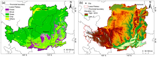
Figure 1.
Study area: (a) Vegetation distribution and administrative countries of the CLP. (b) Elevation and provincial capital cities of the CLP.
2.2. Methodology
The workflow of monitoring and assessing the vegetation health in the CLP can be summarized as follows (see Figure 2). (a) Data preparation. Obtain GPP and Ec data of monthly averages from 2001 to 2020 on the GEE platform. (b) Change detection. Use the BFAST algorithm to detect the short-term disturbance and recovery processes of vegetation and use the BFAST01 algorithm to detect significant breakpoint and long-term trend change. (c) Ecosystem health evaluation. According to the disturbance information, the number of disturbances was extracted and the recovery rate after disturbance was calculated. According to the two segments before and after the significance breakpoint, the trend of change was fitted, and the type of change was divided. The spatial-temporal changes of three health evaluation indexes were analyzed to reveal the variation of health changes.
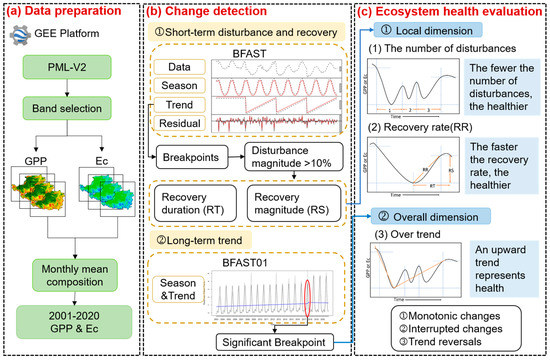
Figure 2.
Workflow of the research method applied in this study; Google Earth Engine, GEE.
2.2.1. Data Preparation
The 500 m and 8-days PML-V2 data from the Google Earth Engine (GEE) platform (https://earthengine.google.org/ (accessed on 23 August 2022)) were used to obtain the monthly gross primary productivity and vegetation evapotranspiration index [36]. The PML-V2 data is based on the Penman–Monteith–Leuning (PML) model, with MODIS and Global Land Data Assistance System (GLDAS) metrological forcing data as input data. The 8-day data of 95 flux towers were used to verify the PML-V2 data. The results show that the Root Mean Square Errors of terrestrial evapotranspiration (ET) and GPP are 0.69 mm d−1 and 1.99 g Cm−2d−1, respectively, and the Bias are −1.8% and 4.2%, respectively [36]. The PML-V2 data contains 5 bands in total, namely gross primary productivity (GPP), vegetation transpiration (Ec), soil evaporation (Es), vegetation canopy interception evaporation (Ei), and ice, snow, water evaporation (ET_water), where [36], among the three components, Ec is coupled with GPP, forming the two dominant processes in global water and carbon cycles. In this study, we chose bands GPP and Ec.
2.2.2. Detecting Vegetation Change
Vegetation changes include short-term abrupt changes and long-term trend changes. In this study, the BFAST algorithm was used to detect short-term changes in vegetation, and the BFAST01 algorithm was used to detect long-term trend changes in vegetation.
- (1)
- BFAST method for short-term abrupt change
The BFAST algorithm utilizes piecewise linear trend and seasonal models to decompose time series into trend, seasonal, and residual components, and can detect abrupt changes in trend and seasonal components [23]. Assuming that an additive decomposition model can iterate into a piecewise linear model that matches trend and seasonality, the algorithm of the model is of the form:
where is the observation data of t, is the trend component, is the seasonal component, and is the remainder component which contains the variation beyond what is explained by and . It is assumed that is piecewise linear, with breakpoints and define , so that
where and are intercept and slope of the piecewise linear, respectively. For and where . and can be used to obtain the magnitude and direction of the abrupt change:
The seasonal component can be characterized as below:
where is amplitudes, is phases, is observation, and represents the order of the harmonic term. Furthermore, the seasonal breakpoints may occur at different times from the breakpoints detected in the trend component. Once the model is fitted, the breakpoint(s) is detected based on computing of residuals at time t as a form of:
where represents the length of the time series, the user-defined value is the minimal time length of a trend segment in fitting the model, is the length of the moving windows. and are actual and expected observation, respectively, so gives OLSs residual, and is their standard deviation. If the model remains stable, the should be close to zero and only fluctuate randomly. However, if a structural change occurs, the will systematically deviate from zero. If deviate from zero beyond a 95% significance boundary, a structural change has occurred and it is considered as a breakpoint.
- (2)
- BFAST01 method for long-term trend
The BFAST01 algorithm is an adjusted version of the season-trend model, designed to detect the most important trend shift in the time series, calculated with either 0 or 1 breakpoint from the moving sum of OLS residuals. BFAST01 offers an effective and comprehensive change detection method for the assessment of major turning points in long-term seasonal and interannual variability as well as important disturbance events [37]. The algorithmic form of the model is as follows:
where the intercept, slope (i.e., trend), amplitudes,…, and phases ,…, (i.e., season) are the unknown parameters, is the known frequency (e.g., = 12 annual observations for a monthly time series), and is the unobservable error term at time t (with standard deviation ).
The BFAST01 algorithm is a simplified variant of BFAST and seeks the major change in the time series. These two models are analogs to each other; however, two important differences exist between them. (1) unlike BFAST, BFAST01 fits a season-trend model to the data to detect only major changes while ignoring small structural changes. (2) BFAST separately and iteratively applies first a seasonal and then a trend model while BFAST01 takes both together into account simultaneously [38]. BFAST and BFAST01 need to be run in the R environment, and the related packages can be downloaded from https://mirrors.tuna.tsinghua.edu.cn/CRAN/ (accessed on 14 February 2022).
The trend types of the whole time series is divided according to the trend before and after a significant mutation point in the time series (Table 1). There are three major types of change patterns (Figure 3), including monotonic changes (increase or decrease), interrupted changes (increase or decrease with interruption), and trend reversals (decrease to increase or increase to decrease).

Table 1.
Descriptions of trend Types.
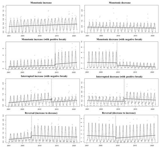
Figure 3.
Examples of trend types: type 1, monotonic increase; type 2, monotonic decrease; type 3, monotonic increase (with positive break); type 4, monotonic decrease (with negative break); type 5, interrupted increase (with negative break); type 6, interrupted decrease (with positive break); type 7, reversal: increase to decrease; type 8, reversal: decrease to increase.
2.2.3. Establishing Indicators for Ecosystem Health
In this study, indicators of ecological health have been quantified statistically from the number of disturbances, recovery rate, and overall trends. The following table shows the indicators used to evaluate ecosystem health (Table 2).
Table 2.
Indicators used to evaluate ecosystem health based on GPP and Ec time series.
- (1)
- The number of disturbances for local dimensional evaluation
A relatively stable ecosystem has a strong ability to maintain its own state when disturbed. Therefore, the greater the number of disturbances, the poorer the ecosystem stability and health [14]. The number of changes can be directly obtained using BFAST algorithm, but the number of disturbances can’t be obtained since the BFAST algorithm can only obtain the magnitude and direction of the disturbance; it cannot directly obtain the disturbance and recovery events. In this study, we extracted changes with a disturbance amplitude greater than 10% (the value of GPP or Ec decreased by at least 10% after disturbance) [14] and calculated the cumulative number of disturbances (Table 2).
- (2)
- Recovery rate for local dimensional evaluation
The resilience represents the ability to recover to the initial state after disturbance. The recovery rate represents the resilience of an ecosystem after being disturbed. The faster the recovery rate, the stronger the resilience and the healthier the ecosystem [14,17,18]. According to slope of linear trend in the segment succeeding the “breakpoint,” we obtain the recovery duration and the recovery amplitude, then calculate the recovery rate, which represents the resilience. The formula and expression (Table 2) are as follows:
where is recovery rate, represents the recovery amplitude, which is obtained according to the amplitude at the end of the disturbance and the end of the recovery; represents the period of from disturbance end to recovery end.
- (3)
- Overall trends for overall dimensional evaluation
The overall trend represents the past and present state of health, reveals the process of health change, and can also predict the future change to a certain extent. The upward trend of GPP and Ec can represent the enhancement of vegetation carbon storage capacity (Table 2), the enhancement of evapotranspiration. The increasing trend of GPP and Ec indicates the improvement of vegetation function and ecosystem health [39,40,41,42], and the downward trend represents the degradation of vegetation function and an unhealthy ecosystem.
3. Results
3.1. Local Dimension Characteristics of Ecosystem Health
By using the BFAST algorithm, we obtained indicators describing the local dimension characteristics of ecosystem health, including the number of disturbances and the recovery rate.
- (1)
- The number of disturbances
In this study, the change of GPP and Ec values that decreased by more than 10% was extracted to obtain the number of disturbances. From 2001 to 2020, pixels experienced between zero and four breakpoints. Since the number of pixels with four breakpoints is less than 5, we ignored the statistical analysis of the pixels with it. As for disturbance pixels of Ec (Figure 4a), 94.4% disturbance pixels had one breakpoint, followed by two breakpoints (5.51%) and three breakpoints (0.1%). A total of 93.11% disturbance pixels of GPP had one breakpoint (Figure 4b), followed by two breakpoints (6.74%) and three breakpoints (0.15%). The spatial disturbance of the number of breakpoints shows a large variability, with all breakpoint classes having discrete disturbances.
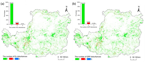
Figure 4.
Spatial distribution of the number of disturbances in the CLP and the percentage of different number of disturbances: (a) Ec; (b) GPP. In both graphs and maps, the green part represents the proportion and spatial distribution of pixels that experienced one breakpoint; the red part represents the pixels that experienced two breakpoints; and the blue part represents the pixels that experienced three breakpoints.
- (2)
- Recovery rate
We only calculated the recovery rate after the first disturbance because most pixels are disturbed once; only a small part of pixels are disturbed between two and four times. Figure 5a shows the rate of recovery for GPP. The maximum percentage of each of recovery classification is 0–0.0015 (43.56%), followed by −0.0007–0 and 0.00015–0.0006 (28.09% and 23.67%). Overall, 70.44% pixels of GPP have recovered after disturbance. Figure 5b shows the rate of recovery for Ec. A total of 63.8% of pixels in each of recovery classification is 0–0.0015, followed by −0.0007–0 (32.91%). Overall, 67.04% pixels of Ec have recovered after disturbance. These results show that most of the vegetation recovered after the disturbance, but the recovery rate was slow.
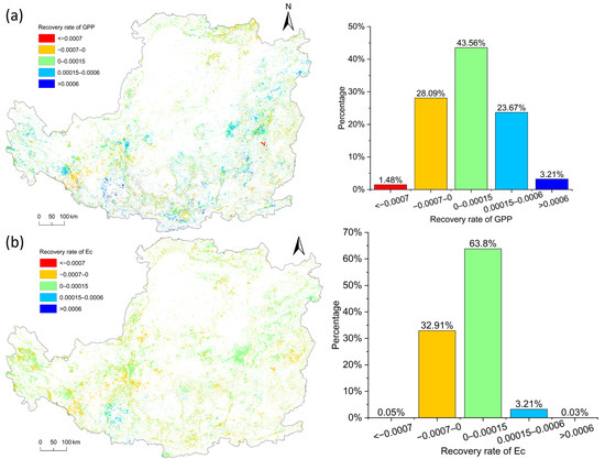
Figure 5.
Spatial distribution of the recovery rate and the percentage of different intervals of the recovery rate: (a) GPP; (b) Ec.
From the results of the local dimensional health indicators we can see, the vegetation on the CLP is not susceptible to multiple disturbances and more than half of the vegetation recovered after the disturbance, but the recovery rate after disturbances is slow. This indicates that the vegetation has weak resilience, and the ecosystem health is very poor.
3.2. Overall Dimension Characteristics of Ecosystem Health
In this study, eight change types of GPP and Ec were obtained by using the BFAST01 algorithm (Figure 3). We analyzed change types of GPP and Ec respectively; type 1 and type 2 were monotone types with no breakpoint, so there was no corresponding break time. The percentage of trend types of GPP are shown in Figure 6. Overall, 37.87% pixels are type 3, followed by type 8 (23.21%) and type 7 (19.22%). Overall, the rise trend type of the GPP accounts for 71.78%, and the decline trend type accounts for 28.22%. Spatially, type 3 was mainly distributed in the northeast and southwest of the CLP and was concentrated in the center of the CLP. Type 7 was mainly distributed in the southern part of Shanxi Province.
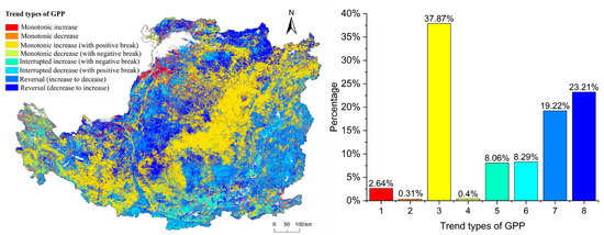
Figure 6.
Spatial distribution and the percentage of different types of GPP.
The percentage of Ec trend types are shown in Figure 7. The maximum percentage of Ec trend type is type 3 (48.02%), followed by type 7 (26.58%). The minimum percentage of trend type is type 4 (0.23%), followed by type 1 (0.99%). Overall, the rising trend type of the Ec accounts for 66.66%, and the decline trend type accounts for 33.34%. Spatially, type 3 is mainly distributed in the northeast and southwest of the CLP and is concentrated in the north of Shanxi Province.
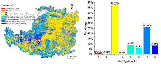
Figure 7.
Spatial distribution and the percentage of different types of Ec.
From the result of overall dimensional health indicators that we can see, most of the vegetation growth is trending toward to a good development, and the ecosystem health has been improved.
4. Discussion
4.1. Multi-dimensional Evaluation for Ecosystem Health
The difference between this study and previous studies is that a multi-dimensional health assessment method was proposed to evaluate the health of the CLP from the perspective of the local and overall dimensions. Previous studies have mostly diagnosed the health of the ecosystem only through its response to disturbances. However, ecosystem health is a multidimensional definition [43], with both short-term change and long-term change. This study can evaluate ecological health more comprehensively and obtain more accurate evaluation results.
We selected GPP and Ec to represent the carbon storage capacity and water condition of vegetation in semi-arid areas. In terms of overall indicators, we selected the overall trend as the indicator. The rising trend of GPP and Ec could represent both the enhancement of carbon storage capacity and the enhancement of transpiration of sufficient water. As for the local dimension health index, we selected the number of disturbances and recovery rate. The disturbance will cause vegetation change, which can be divided into natural disturbance and anthropogenic disturbance. Anthropogenic disturbances, such as changes in farmland that are caused by harvesting, changes in grassland that are caused by overgrazing, and changes in land use patterns that are caused by urbanization, as well as natural disturbances such as decreased precipitation and CO2 concentrations, all lead to decreases in GPP and Ec [44,45,46,47,48,49,50,51,52]. Therefore, the small disturbance frequency represents ecological health. The recovery rate of GPP and Ec can correspond to the ability of vegetation to recover from disturbance, rapid recovery represents rapid vegetation growth, suitable water conditions, and enhanced evapotranspiration.
Therefore, this study was able to obtain the disturbance of vegetation caused by anthropogenic and environmental factors in the local dimension, and the change of carbon storage and water production capacity of vegetation after the disturbance. In the overall dimension, the change of vegetation growth and the improvement or degradation of ecosystem function are obtained. In conclusion, the combination of the local dimension and overall dimension analysis can comprehensively reveal the CLP’s vegetation health during the past two decades. This method will open new perspectives and generate new knowledge about vegetation health in the CLP.
4.2. The Analysis of Ecosystem Health
Our results showed that more than 90% of disturbance pixels of GPP and Ec in the short-term change only once (Figure 4), and that more than 60% of pixels recover after disturbance. However, the recovery rate after disturbance is slow, and the interval with the largest proportion is 0–0.00015 (Figure 5). This indicates that the vegetation resilience of the CLP is poor, and that the ecological environment is still fragile. In terms of overall dimension, we found that more than 60% of GPP and Ec pixels showed an upward trend during the past two decades, and among them, most exhibited monotonic increasing trends (Figure 6, Figure 7). This trend is consistent with previous studies [40,41,53,54].
The results illustrated that the function of the ecosystem on the CLP has been improved, but the resilience of vegetation is weak. Overall, the health of the ecosystem has been improved, but locally, the ecosystem is not healthy. This phenomenon may be attributed to ecological restoration projects such as the “Grain for Green” program, “Natural Forest Conservation” program and “Three Norths Shelter Forest System” [55]. Between 1999 and 2013, the vegetation cover of the CLP almost doubled from 31.6% to 59.6% [56]. The change of land cover type enhanced the carbon storage capacity and transpiration of vegetation, and the GPP and Ec increased significantly in the CLP. However, the availability of water is the biggest factor restricting the growth and survival of vegetation in the CLP; unreasonable planting strategies increase water consumption in the area, and the decline in the groundwater level eventually results in slow growth or death of vegetation [57]. At the same time, there is a single vegetation species on the CLP, so the ability to recover from disturbance may be weak [56].
4.3. Limitation and Outlook
Although the multi-dimensional health assessment method was proposed in this study, a relatively comprehensive evaluation was made on the CLP ecosystem from the overall and local dimensions. There are still limitations in this study. The focus of this study is to evaluate ecosystem health based on the spatiotemporal changes of ecological function indicators, without paying too much attention to health-influencing factors, such as the reasons for the changes in the three health indicators and the reasons for the occurrence of significant breakpoints in the trend. Therefore, the next step in this study is to analyze the driving forces of health change in combination with high-resolution data and other ancillary data. Imagery from Landsat with finer spatial resolution may be a good choice, there would be a great advantage obtained by combining PML-V2 and Landsat data for small-scale disturbances monitoring, and then analyzing the influencing factors of ecosystem health changes at multiple spatial scales. In addition, landcover data, DEM data, and precipitation data can be combined to analyze the relationship between ecosystem health and vegetation types, as well as topography and climate.
5. Conclusions
In this study, an attempt was made to evaluate vegetation health in the CLP in multi-dimensional analysis using GPP and Ec time series data. The short-term abrupt change (disturbance time and recovery rate) and long-term trend change (eight change types) were researched to describe and quantify the vegetation health between 2001 and 2020. BFAST and BFAST01 algorithms were used to obtain the three ecological health assessment indicators. The most important findings and conclusions drawn from this study include the following.
- (1)
- More than 90% of disturbance pixels of GPP and Ec in the short-term change only once and more than 60% of pixels recover after disturbance. However, the recovery rate after disturbance is slow, and the interval with the largest proportion is 0–0.00015. The long-term trend mostly exhibited a monotonic increasing trend.
- (2)
- The function of the ecosystem on the CLP has been improved, but the resilience of vegetation is weak. Overall, the health of the ecosystem has been improved, but locally, the ecosystem is not healthy.
Therefore, we suggest that the ecological restoration project of the CLP should shift its focus from increasing the amount of vegetation to enhancing its resilience.
Author Contributions
Conceptualization, X.L. (Xiangnan Liu) and X.L. (Xiaoyue Li); methodology, B.H. and X.L. (Xiaoyue Li); validation, L.T., Q.Y., L.Z. and Y.M.; writing—original draft preparation, X.L. (Xiaoyue Li); visualization, X.L. (Xiaoyue Li); supervision, X.L. (Xiangnan Liu); All authors have read and agreed to the published version of the manuscript.
Funding
This work was supported by the Flexible Introduction Team of Ningxia Hui Autonomous Region (Grant No. 2020RXTDLX03); Remote sensing monitoring and evaluation of ecological status in Ningxia (Grant No. NXCZ20220203).
Acknowledgments
The authors would like to thank the anonymous reviewers and the editor for their constructive.
Conflicts of Interest
The authors declare no conflict of interest.
References
- Fang, W.; Huang, S.; Huang, Q.; Huang, G.; Wang, H.; Leng, G.; Wang, L.; Guo, Y. Probabilistic Assessment of Remote Sensing-Based Terrestrial Vegetation Vulnerability to Drought Stress of the Loess Plateau in China. Remote Sens. Environ. 2019, 232, 111290. [Google Scholar] [CrossRef]
- Feng, X.; Fu, B.; Piao, S.; Wang, S.; Ciais, P.; Zeng, Z.; Lü, Y.; Zeng, Y.; Li, Y.; Jiang, X.; et al. Revegetation in China’s Loess Plateau Is Approaching Sustainable Water Resource Limits. Nat. Clim. Change 2016, 6, 1019–1022. [Google Scholar] [CrossRef]
- He, L.; Guo, J.; Jiang, Q.; Zhang, Z.; Yu, S. How Did the Chinese Loess Plateau Turn Green from 2001 to 2020? An Explanation Using Satellite Data. CATENA 2022, 214, 106246. [Google Scholar] [CrossRef]
- Cao, S.; Chen, L.; Yu, X. Impact of China’s Grain for Green Project on the Landscape of Vulnerable Arid and Semi-Arid Agricultural Regions: A Case Study in Northern Shaanxi Province. J. Appl. Ecol. 2009, 46, 536–543. [Google Scholar] [CrossRef]
- Liu, W.; Sun, F.; Sun, S.; Guo, L.; Wang, H.; Cui, H. Multi-Scale Assessment of Eco-Hydrological Resilience to Drought in China over the Last Three Decades. Sci. Total Environ. 2019, 672, 201–211. [Google Scholar] [CrossRef] [PubMed]
- Zhang, Y.; Peng, C.; Li, W.; Tian, L.; Zhu, Q.; Chen, H.; Fang, X.; Zhang, G.; Liu, G.; Mu, X.; et al. Multiple Afforestation Programs Accelerate the Greenness in the ‘Three North’ Region of China from 1982 to 2013. Ecol. Indic. 2016, 61, 404–412. [Google Scholar] [CrossRef]
- Cao, S.; Chen, L.; Shankman, D.; Wang, C.; Wang, X.; Zhang, H. Excessive Reliance on Afforestation in China’s Arid and Semi-Arid Regions: Lessons in Ecological Restoration. Earth-Sci. Rev. 2011, 104, 240–245. [Google Scholar] [CrossRef]
- Li, J.; Peng, S.; Li, Z. Detecting and Attributing Vegetation Changes on China’s Loess Plateau. Agric. For. Meteorol. 2017, 247, 260–270. [Google Scholar] [CrossRef]
- Han, Q.; Zhang, J.; Shi, X.; Zhou, D.; Ding, Y.; Peng, S. Ecological Function-Oriented Vegetation Protection and Restoration Strategies in China’s Loess Plateau. J. Environ. Manage. 2022, 323, 116290. [Google Scholar] [CrossRef] [PubMed]
- Rapport, D.J.; Regier, H.A.; Hutchinson, T.C. Ecosystem Behavior Under Stress. Am. Nat. 1985, 125, 617–640. [Google Scholar] [CrossRef]
- He, J.; Pan, Z.; Liu, D.; Guo, X. Exploring the Regional Differences of Ecosystem Health and Its Driving Factors in China. Sci. Total Environ. 2019, 673, 553–564. [Google Scholar] [CrossRef]
- Woodcock, C.E.; Loveland, T.R.; Herold, M.; Bauer, M.E. Transitioning from Change Detection to Monitoring with Remote Sensing: A Paradigm Shift. Remote Sens. Environ. 2020, 238, 111558. [Google Scholar] [CrossRef]
- Liu, F.; Liu, H.; Xu, C.; Shi, L.; Zhu, X.; Qi, Y.; He, W. Old-growth Forests Show Low Canopy Resilience to Droughts at the Southern Edge of the Taiga. Glob. Change Biol. 2021, 27, 2392–2402. [Google Scholar] [CrossRef] [PubMed]
- von Keyserlingk, J.; de Hoop, M.; Mayor, A.G.; Dekker, S.C.; Rietkerk, M.; Foerster, S. Resilience of Vegetation to Drought: Studying the Effect of Grazing in a Mediterranean Rangeland Using Satellite Time Series. Remote Sens. Environ. 2021, 255, 112270. [Google Scholar] [CrossRef]
- Yao, Y.; Fu, B.; Liu, Y.; Li, Y.; Wang, S.; Zhan, T.; Wang, Y.; Gao, D. Evaluation of Ecosystem Resilience to Drought Based on Drought Intensity and Recovery Time. Agric. For. Meteorol. 2022, 314, 108809. [Google Scholar] [CrossRef]
- Holling, C.S. Resilience and Stability of Ecological Systems. Annu. Rev. Ecol. Evol. Syst. 1973, 4, 1–23. [Google Scholar] [CrossRef]
- Huang, Z.; Liu, X.; Yang, Q.; Meng, Y.; Zhu, L.; Zou, X. Quantifying the Spatiotemporal Characteristics of Multi-Dimensional Karst Ecosystem Stability with Landsat Time Series in Southwest China. Int. J. Appl. Earth Obs. Geoinf. 2021, 104, 102575. [Google Scholar] [CrossRef]
- Liu, M.; Liu, X.; Wu, L.; Tang, Y.; Li, Y.; Zhang, Y.; Ye, L.; Zhang, B. Establishing Forest Resilience Indicators in the Hilly Red Soil Region of Southern China from Vegetation Greenness and Landscape Metrics Using Dense Landsat Time Series. Ecol. Indic. 2021, 121, 106985. [Google Scholar] [CrossRef]
- Zhu, Z.; Woodcock, C.E. Continuous Change Detection and Classification of Land Cover Using All Available Landsat Data. Remote Sens. Environ. 2014, 144, 152–171. [Google Scholar] [CrossRef]
- Zhu, Z.; Zhang, J.; Yang, Z.; Aljaddani, A.H.; Cohen, W.B.; Qiu, S.; Zhou, C. Continuous Monitoring of Land Disturbance Based on Landsat Time Series. Remote Sens. Environ. 2020, 238, 111116. [Google Scholar] [CrossRef]
- Kennedy, R.E.; Yang, Z.; Cohen, W.B. Detecting Trends in Forest Disturbance and Recovery Using Yearly Landsat Time Series: 1. LandTrendr—Temporal Segmentation Algorithms. Remote Sens. Environ. 2010, 114, 2897–2910. [Google Scholar] [CrossRef]
- Meng, Y.; Liu, X.; Wang, Z.; Ding, C.; Zhu, L. How Can Spatial Structural Metrics Improve the Accuracy of Forest Disturbance and Recovery Detection Using Dense Landsat Time Series? Ecol. Indic. 2021, 132, 108336. [Google Scholar] [CrossRef]
- Verbesselt, J.; Hyndman, R.; Newnham, G.; Culvenor, D. Detecting Trend and Seasonal Changes in Satellite Image Time Series. Remote Sens. Environ. 2010, 114, 106–115. [Google Scholar] [CrossRef]
- Huang, C.; Goward, S.N.; Masek, J.G.; Thomas, N.; Zhu, Z.; Vogelmann, J.E. An Automated Approach for Reconstructing Recent Forest Disturbance History Using Dense Landsat Time Series Stacks. Remote Sens. Environ. 2010, 114, 183–198. [Google Scholar] [CrossRef]
- Browning, D.M.; Maynard, J.J.; Karl, J.W.; Peters, D.C. Breaks in MODIS Time Series Portend Vegetation Change: Verification Using Long-Term Data in an Arid Grassland Ecosystem. Ecol. Appl. 2017, 27, 1677–1693. [Google Scholar] [CrossRef] [PubMed]
- Watts, L.M.; Laffan, S.W. Effectiveness of the BFAST Algorithm for Detecting Vegetation Response Patterns in a Semi-Arid Region. Remote Sens. Environ. 2014, 154, 234–245. [Google Scholar] [CrossRef]
- Jong, R.; Verbesselt, J.; Schaepman, M.E.; Bruin, S. Trend Changes in Global Greening and Browning: Contribution of Short-Term Trends to Longer-Term Change. Glob. Change Biol. 2012, 18, 642–655. [Google Scholar] [CrossRef]
- Hirsch, R.M.; Slack, J.R.; Smith, R.A. Techniques of Trend Analysis for Monthly Water Quality Data. Water Resour. Res. 1982, 18, 107–121. [Google Scholar] [CrossRef]
- Hirsch, R.M.; Slack, J.R. A Nonparametric Trend Test for Seasonal Data With Serial Dependence. Water Resour. Res. 1984, 20, 727–732. [Google Scholar] [CrossRef]
- Sen, P.K. Estimates of the Regression Coefficient Based on Kendall’s Tau. J. Am. Stat. Assoc. 1968, 63, 1379–1389. [Google Scholar] [CrossRef]
- Fensholt, R.; Langanke, T.; Rasmussen, K.; Reenberg, A.; Prince, S.D.; Tucker, C.; Scholes, R.J.; Le, Q.B.; Bondeau, A.; Eastman, R.; et al. Greenness in Semi-Arid Areas across the Globe 1981–2007—an Earth Observing Satellite Based Analysis of Trends and Drivers. Remote Sens. Environ. 2012, 121, 144–158. [Google Scholar] [CrossRef]
- Pan, N.; Feng, X.; Fu, B.; Wang, S.; Ji, F.; Pan, S. Increasing Global Vegetation Browning Hidden in Overall Vegetation Greening: Insights from Time-Varying Trends. Remote Sens. Environ. 2018, 214, 59–72. [Google Scholar] [CrossRef]
- Bernardino, P.N.; De Keersmaecker, W.; Fensholt, R.; Verbesselt, J.; Somers, B.; Horion, S. Global-scale Characterization of Turning Points in Arid and Semi-arid Ecosystem Functioning. Glob. Ecol. Biogeogr. 2020, 29, 1230–1245. [Google Scholar] [CrossRef]
- Yang, Q.; Liu, X.; Huang, Z.; Guo, B.; Tian, L.; Wei, C.; Meng, Y.; Zhang, Y. Integrating Satellite-Based Passive Microwave and Optically Sensed Observations to Evaluating the Spatio-Temporal Dynamics of Vegetation Health in the Red Soil Regions of Southern China. GIScience Remote Sens. 2022, 59, 215–233. [Google Scholar] [CrossRef]
- Smith, W.K.; Dannenberg, M.P.; Yan, D.; Herrmann, S.; Barnes, M.L.; Barron-Gafford, G.A.; Biederman, J.A.; Ferrenberg, S.; Fox, A.M.; Hudson, A.; et al. Remote Sensing of Dryland Ecosystem Structure and Function: Progress, Challenges, and Opportunities. Remote Sens. Environ. 2019, 233, 111401. [Google Scholar] [CrossRef]
- Zhang, Y.; Kong, D.; Gan, R.; Chiew, F.H.S.; McVicar, T.R.; Zhang, Q.; Yang, Y. Coupled Estimation of 500 m and 8-Day Resolution Global Evapotranspiration and Gross Primary Production in 2002–2017. Remote Sens. Environ. 2019, 222, 165–182. [Google Scholar] [CrossRef]
- de Jong, R.; Verbesselt, J.; Zeileis, A.; Schaepman, M. Shifts in Global Vegetation Activity Trends. Remote Sens. 2013, 5, 1117–1133. [Google Scholar] [CrossRef]
- Brakhasi, F.; Hajeb, M.; Mielonen, T.; Matkan, A.; Verbesselt, J. Investigating Aerosol Vertical Distribution Using CALIPSO Time Series over the Middle East and North Africa (MENA), Europe, and India: A BFAST-Based Gradual and Abrupt Change Detection. Remote Sens. Environ. 2021, 264, 112619. [Google Scholar] [CrossRef]
- Li, W.; Chen, D. Changes in Gross Primary Production in Response to Afforestation in the Hilly Loess Plateau of Northern Shaanxi, China. Forests 2022, 13, 1414. [Google Scholar] [CrossRef]
- Ma, J.; Xiao, X.; Miao, R.; Li, Y.; Chen, B.; Zhang, Y.; Zhao, B. Trends and Controls of Terrestrial Gross Primary Productivity of China during 2000–2016. Environ. Res. Lett. 2019, 14, 084032. [Google Scholar] [CrossRef]
- Sun, M.; Dong, Q.; Jiao, M.; Zhao, X.; Gao, X.; Wu, P.; Wang, A. Estimation of Actual Evapotranspiration in a Semiarid Region Based on GRACE Gravity Satellite Data—A Case Study in Loess Plateau. Remote Sens. 2018, 10, 2032. [Google Scholar] [CrossRef]
- Ma, Z.; Yan, N.; Wu, B.; Stein, A.; Zhu, W.; Zeng, H. Variation in Actual Evapotranspiration Following Changes in Climate and Vegetation Cover during an Ecological Restoration Period (2000–2015) in the Loess Plateau, China. Sci. Total Environ. 2019, 689, 534–545. [Google Scholar] [CrossRef]
- Tett, P.; Gowen, R.; Painting, S.; Elliott, M.; Forster, R.; Mills, D.; Bresnan, E.; Capuzzo, E.; Fernandes, T.; Foden, J.; et al. Framework for Understanding Marine Ecosystem Health. Mar. Ecol. Prog. Ser. 2013, 494, 1–27. [Google Scholar] [CrossRef]
- Bai, M.; Mo, X.; Liu, S.; Hu, S. Contributions of Climate Change and Vegetation Greening to Evapotranspiration Trend in a Typical Hilly-Gully Basin on the Loess Plateau, China. Sci. Total Environ. 2019, 657, 325–339. [Google Scholar] [CrossRef]
- Deng, L.; Liu, G.; Shangguan, Z. Land-Use Conversion and Changing Soil Carbon Stocks in China’s ‘Grain-for-Green’ Program: A Synthesis. Glob. Change Biol. 2014, 20, 3544–3556. [Google Scholar] [CrossRef]
- Li, G.; Zhang, F.; Jing, Y.; Liu, Y.; Sun, G. Response of Evapotranspiration to Changes in Land Use and Land Cover and Climate in China during 2001-2013. Sci. Total Environ. 2017, 596-597, 256–265. [Google Scholar] [CrossRef]
- Fang, B.; Lei, H.; Zhang, Y.; Quan, Q.; Yang, D. Spatio-Temporal Patterns of Evapotranspiration Based on Upscaling Eddy Covariance Measurements in the Dryland of the North China Plain. Agric. For. Meteorol. 2020, 281, 107844. [Google Scholar] [CrossRef]
- Zhao, A.; Yu, Q.; Wang, D.; Zhang, A. Spatiotemporal Dynamics of Ecosystem Water Use Efficiency over the Chinese Loess Plateau Base on Long-Time Satellite Data. Environ. Sci. Pollut. Res. 2022, 29, 2298–2310. [Google Scholar] [CrossRef]
- Bo, Y.; Li, X.; Liu, K.; Wang, S.; Zhang, H.; Gao, X.; Zhang, X. Three Decades of Gross Primary Production (GPP) in China: Variations, Trends, Attributions, and Prediction Inferred from Multiple Datasets and Time Series Modeling. Remote Sens. 2022, 14, 2564. [Google Scholar] [CrossRef]
- Xu, S.; Yu, Z.; Yang, C.; Ji, X.; Zhang, K. Trends in Evapotranspiration and Their Responses to Climate Change and Vegetation Greening over the Upper Reaches of the Yellow River Basin. Agric. For. Meteorol. 2018, 263, 118–129. [Google Scholar] [CrossRef]
- Deng, C.; Zhang, B.; Cheng, L.; Hu, L.; Chen, F. Vegetation Dynamics and Their Effects on Surface Water-Energy Balance over the Three-North Region of China. Agric. For. Meteorol. 2019, 275, 79–90. [Google Scholar] [CrossRef]
- Zhang, K.; Kimball, J.S.; Nemani, R.R.; Running, S.W.; Hong, Y.; Gourley, J.J.; Yu, Z. Vegetation Greening and Climate Change Promote Multidecadal Rises of Global Land Evapotranspiration. Sci. Rep. 2015, 5, 15956. [Google Scholar] [CrossRef]
- He, P.; Sun, Z.; Xu, D.; Liu, H.; Yao, R.; Ma, J. Combining Gradual and Abrupt Analysis to Detect Variation of Vegetation Greenness on the Loess Areas of China. Front. Earth Sci. 2022, 16, 368–380. [Google Scholar] [CrossRef]
- Li, C.; Zhang, Y.; Shen, Y.; Kong, D.; Zhou, X. LUCC-Driven Changes in Gross Primary Production and Actual Evapotranspiration in Northern China. J. Geophys. Res. Atmos. 2020, 125. [Google Scholar] [CrossRef]
- Lu, F.; Hu, H.; Sun, W.; Zhu, J.; Liu, G.; Zhou, W.; Zhang, Q.; Shi, P.; Liu, X.; Wu, X.; et al. Effects of National Ecological Restoration Projects on Carbon Sequestration in China from 2001 to 2010. Proc. Natl. Acad. Sci. USA 2018, 115, 4039–4044. [Google Scholar] [CrossRef]
- Bryan, B.A.; Gao, L.; Ye, Y.; Sun, X.; Connor, J.D.; Crossman, N.D.; Stafford-Smith, M.; Wu, J.; He, C.; Yu, D.; et al. China’s Response to a National Land-System Sustainability Emergency. Nature 2018, 559, 193–204. [Google Scholar] [CrossRef]
- Cao, D.; Zhang, J.; Xun, L.; Yang, S.; Wang, J.; Yao, F. Spatiotemporal Variations of Global Terrestrial Vegetation Climate Potential Productivity under Climate Change. Sci. Total Environ. 2021, 770, 145320. [Google Scholar] [CrossRef]


Disclaimer/Publisher’s Note: The statements, opinions and data contained in all publications are solely those of the individual author(s) and contributor(s) and not of MDPI and/or the editor(s). MDPI and/or the editor(s) disclaim responsibility for any injury to people or property resulting from any ideas, methods, instructions or products referred to in the content. |
© 2023 by the authors. Licensee MDPI, Basel, Switzerland. This article is an open access article distributed under the terms and conditions of the Creative Commons Attribution (CC BY) license (https://creativecommons.org/licenses/by/4.0/).