Abstract
The ancient Aniangzhai (ANZ) landslide in Danba County, Sichuan Province of southwest China was reactivated after a series of complex hazard events that occurred in June 2020. Since then, and until June 2021, emergency engineering work was carried out to prevent the further failure of the reactivated landslide. This study investigates the potential of joint use of time series Interferometric Synthetic Aperture Radar (InSAR) and optical pixel offset tracking (POT) to assess deformation characteristic and spatial-temporal evolution of the reactivated ANZ landslide during the post-failure stage. The relationships between sun illumination differences, temporal baseline of correlation pairs and the uncertainties were deeply explored. Surface deformation along the line-of-sight (LoS) direction was retrieved by the time series InSAR processing with the two Sentinel-1 datasets, revealing a maximum deformation rate up to 190 mm/year. The large horizontal displacements were also detected from the POT processing using 11 optical images acquired by the PlanetScope satellite (3 m spatial resolution), showing a significant increase of about 24 m between 24 June 2020 and 11 June 2021. The time series analysis from the InSAR and optical POT results revealed that the reactivated ANZ landslide body is gradually slowing down to a steady deformation status since its occurrence in August 2020, indicating the effectiveness of engineering work on the prevention of further landslide. A slight acceleration was detected from both InSAR and optical POT time series analysis between May 2021 and June 2021, which could be caused by the increased rainfall in May 2021.
1. Introduction
In a narrow river valley, debris flows or landslides may obstruct rivers and cause landslide dams [1,2]. These landslide dams represent unconsolidated sediments that can be reactivated or cause other dams to reactivate [3,4] and thus pose a significant hazard to life and infrastructure along the river valley. Therefore, it is of importance to carefully monitor the potential for existing landslide bodies to reactivate, taking into account the influence of weather on the body [5].
The ancient Aniangzhai Landslide in Danba County, in the Sichuan Province of China, was reactivated on 17 June 2020 after a complex multi-hazard chain initially triggered by heavy midnight rainfall. Intense rainfall triggered the Meilong debris flow on the right bank of the Xiaojinchuan River, blocking the river and forming a dammed lake [6,7]. Many houses in the Guanzhou Village were submerged, and the national highway G350 was blocked, causing 28 casualties and the evacuation of 5800 people upstream [8]. The dammed lake began to breach on the same day and caused an outburst flood. Continuous undercutting and intense erosion by the outburst of debris flow and flooding caused the collapse of the toe section of the ancient ANZ landslide, which in turn resulted in the reactivation of the middle section of the ANZ slope.
Emergency field investigation and monitoring work were undertaken to understand the deformation characteristics and failure mechanism of the reactivated ANZ landslide [6,8]. Emergency engineering work to stabilise the area was carried out between 25 June 2020 and 09 July 2020 [9]. According to the local media news [10], landslide remediation engineering work was also ongoing on the reactivated ANZ landslide. Three major activities were undertaken: Sediment cleaning in the river channel (completed at the end of March 2021); erosion and washing prevention of the riverway (completed in mid-April 2021); and earth backfilling over the slope (completed at the end of April 2021). On 25 June 2022, two large rocks in the landslide top area were removed to prevent additional landslide collapse and Xiaojinchuan River blockage (http://www.sc404.com/new/Article/ShowArticle.asp?ArticleID=671 accessed on 6 November 2022).
Many researchers have conducted post-failure monitoring over the reactivated ANZ landslide to explore the spatial-temporal evolution of the landslide body [6,8,9,11,12]. Post-failure assessments predict that further failure of this reactivated landslide could block the Xiaojinchuan River again and pose a severe threat to the infrastructure and residents downstream. Based on data from a total station over the reactivated ANZ landslide monitored over a period of 20 days (23 June 2020–12 July 2020), Zhao et al. found that the deformation rates in the horizontal and vertical directions over the middle and toe sections decreased gradually and remain at about 5 mm/h [6]. An initial increase in deformation rates was observed over the upstream and downstream sections, but it slowly decreased to a rate of about 5 mm/h toward the end of the observation period [6].
On the other hand, Zhu et al. found a linear deformation trend from the time series of InSAR of the Sentinel-1 data spanning from 20 April 2018 to 20 May 2020, during the pre-failure stage [8]. From the monitoring system network deployed over the slope (20 June 2020 to 22 August 2020), two accelerations were detected on 5 July 2020 and 18 July 2020, respectively, showing a good agreement between surface displacement and rainfall [8]. Similarly, Kuang et al. applied the time series InSAR using both the descending and ascending Sentinel-1 data from March 2018 to July 2020 to explore the surface deformation over the ANZ slope [11]. No apparent deformation changes (precursory deformation) were detected before the multi-hazard chain on 17 June 2020, while evident accelerated deformation was observed over the slope after the event.
Using three-dimensional deformation of the reactivated ANZ landslide based on the integration of terrestrial laser scanning (TLS) and unmanned aerial vehicles (UAV), Jiang et al. (2021) found that the erosion and downcutting of the riverbed by the outburst flood was the main reason for the reactivation of the ancient ANZ landslide, and that the deformation of the landslide body gradually slowed down [13]. Subsequently, Ning et al. explored the evolving process of the reactivated ANZ landslide before and after the emergency engineering measures using ground-based radar monitoring from 18 June 2020 to 20 August 2020. They found that the deformation rate and acceleration of the landslide body were decreased after the engineering work, with two accelerating stages detected in this period [9]. These studies used field survey data, satellite data, and aerial remote sensing data gathered during the post-failure stage (i.e., mainly between June 2020 and August 2020) to perform in-depth investigation on the reactivated ANZ landslide. A series of preventive engineering work continued in 2021, beyond the time frame covered by these studies. The knowledge gained from these studies was insufficient to demonstrate the response of the reactivated ANZ slope to the ongoing engineering work, thus this paper extends the observational time frame up to June 2021, and uses multi-temporal satellite data acquired by SAR and optical sensors to further investigate the post-failure evolution of the reactivated ANZ landslide.
Interferometric Synthetic Aperture Radar (InSAR) is useful for measuring surface deformation along the radar LoS direction with a relatively high accuracy (up to millimetre level) and high spatial resolution in all-weather condition [14]. The time series InSAR technique has been widely applied to landslide mapping and monitoring, including pre-failure analysis and precursor detection [15], landslide detection and inventory [16], post-failure analysis [17], and long-term spatial-temporal evolution [18]. It is sensitive to capture subtle deformation caused by the slow-moving landslides with deformation rates ranging from several millimetres to tens of centimetres each year [19]. However, for fast-moving landslides, especially during the post-failure stage or after the reactivation, large deformation gradients would cause high decorrelation and phase unwrapping error. The optical pixel offset tracking (POT) technique can be used to measure large horizontal displacements caused by the fast-moving landslides [20]. Horizontal displacements over the landslide area can be easily retrieved from sub-pixel images correlation between two optical images acquired on different dates. Sub-pixel image correlation approaches have been successfully applied in various studies of landslide detection and monitoring [21,22].
High-resolution 3D displacements information can be easily retrieved from the use of field data from terrestrial laser scanning or remote sensing data from light detection and ranging (LiDAR) and unmanned aerial vehicles (UAV) [23,24]. For obtaining the real 3D displacements from SAR datasets, SAR displacement measurements from at least three imaging geometries with significant difference are required. At present, two different imaging geometries can be easily obtained from the current SAR satellites, i.e., the descending and ascending InSAR LoS directions with the right-looking mode. Due to its near-polar orbit design, InSAR LoS measurements are sensitive to vertical and East/West displacements, but not to North/South displacements [25]. Therefore, under the assumption that the North/South displacement is negligible, many studies have been carried out to calculate the vertical and East/West displacements by combining the easily acquired descending and ascending InSAR measurements [26,27,28]. However, to obtain the real 3D displacement, at least another displacement measurement must be integrated for complementing the descending and ascending InSAR LoS measurements. Generally, there are mainly two approaches to realize the retrieval of 3D displacements. The first is to integrate left-looking SAR data with right-looking data in both descending and ascending modes. This integration allows for high-accuracy retrieval of 3D displacements using only InSAR measurements but is made difficult by rarity of left-looking SAR data [29,30].
Another approach is to incorporate the azimuth measurement from SAR data with the pixel offset tracking (POT) technique. This technique can measure the displacements along the satellite azimuth direction, which is near the North/South direction. For this case, the accuracy of the POT technique is significantly limited by the low azimuth pixel resolution of Sentinel-1 SAR data. At the same time, the signal-to-noise ratio (SNR) of the POT-derived azimuth displacement measurements was significantly low to detect any meaningful displacement signal due to Sentinel-1 SAR data’s low azimuth pixel resolution. Instead, the PlanetScope optical images with high spatial resolution (3 m) were used for obtaining the POT results with considerable accuracy. Moreover, 2D displacements including the East/West and North/South measurements can be directly derived from the optical POT results, which plays a key role in complementing the displacement measurements along the North/South direction.
Several emergency affairs and engineering work were conducted over this site during the post-event stage, and many on-site monitoring and investigations were conducted to understand the deformation characteristics. However, the temporal coverage and frequency of these works are limited due to high labour cost and complex topography. Satellite remote sensing data were not fully exploited for monitoring the post-failure evolution of this event. Using satellite radar and optical remote sensing data, this study covers the time frame of on-site engineering work for better understanding of post-event deformation characteristics and spatial-temporal evolution at multiple scales. Future engineering works for hazard mitigation for this site and the sites with similar geological conditions could benefit from the outcome of this work.
2. Study Area and Datasets
2.1. Geological Settings
Aniangzhai village in Danba County, where the ANZ landslide occurred, is lying on the central-west section of the Sichuan Province in the southwest part of China, as shown in Figure 1a. This region is located in the transition zone between the Qinghai-Tibetan Plateau and Sichuan Basin, with elevations ranging between 107 and 7473 m above sea level (a.s.l.). Two large active fault belts intersect in this region, the Xianshuihe-Xiaojiang fault belt in the west and the Longmenshan thrust fault belt in the east. This area is seismically active, with multiple historical earthquakes occurring around, including 1933 MW 7.3 Diexi Earthquake on the Songpinggou fault [31], the 1973 MS 7.6 Luhuo Earthquake on the Xianshuihe fault [32], and the 2008 MW 7.9 Wenchuan Earthquake on the Longmenshan fault [33]. This region’s geomorphological setting is characterized by high mountains and river basins, with complicated topography and a wide range of relative heights.
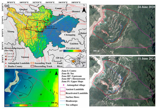
Figure 1.
Geological background of the study area. (a) Regional elevation map; (b) Enlarged view of the ANZ landslide; (c,d) Post-failure true colour optical images collected from the PlanetScope satellite (Table 1 shows technical specifications of the PlanetScope optical images).
The overall topographic setting of the ANZ landslide is shown in Figure 1b. The elevation difference is up to 1000 m from the head to the toe of the ANZ landslide. The ANZ landslide is mainly northwest facing, with an inclination of 50° in the upper section and 20° at the lower part. Based on the landslide features observed from the field investigation and local topography [6,8,34], the ANZ landslide can be divided into four zones: Zone I Centre section, Zone II Toe section, Zone III″ Upstream section, and Zone IV Upper slope section. Note that Zone III can be divided in two parts: Part III′ upstream section and Part III″ downstream section. Part III″ is not a segment of landslide area as it includes a fraction of the bed rock area. Under the joint effect of heavy rainfall, the intense erosion and downcutting by the Xiaojinchuan River and the multi-hazard chain on 17 June 2020, the lower and middle sections of the ancient ANZ landslide were reactivated, and thus named the reactivated ANZ landslide. The length of the reactivated area was up to 700 m, and the width along the river was about 800 m. The front edge of the ANZ landslide formed a steep face with a slope of about 60–70° and a height of 60 m at the toe. In the toe section, the maximum elevation change was up to 61.5 m based on the topographic difference analysis [6]. A relatively gentle slope ranging from 35 to 45° was obtained in the middle and upper sections of the ANZ landslide [7]. This area is characteristic of subtropical monsoon climate, where the average annual temperature is approximately 14.6°. According to the rainfall data recorded from the Danba Meteorological Bureau, the annual rainfall is about 532.7–823.3 mm, 80% of which occurs between May and September [6].
Figure 1c,d presents two post-failure true colour images from PlanetScope satellite collected on 24 June 2020 and 11 June 2021 over the ANZ slope, respectively (Table 1). The image from 24 June 2020, only 1 week after the reactivation of the ANZ landslide, shows the collapsed area at the ancient landslide toe, where three surface flows were detected, with two in the middle and one in the upper slope. The image also shows the head scarps on the top of the reactivated landslide. Figure 1d corresponds to an image acquisition of almost 1 year after the reactivation of the landslide (11 June 2021). It proves that the head scarps on the top dramatically expanded along the downslope, extending down to the toe through the multiple road dislocations upstream. In addition, two surface flows in the middle experienced clear expansion during this period. The ANZ slope mainly moved toward the northwest (downslope) direction, which is demonstrated by the field survey and previous results [6,8,34]. However, no apparent changes were observed for the surface flow on the upper slope of the ancient ANZ landslide.

Table 1.
Basic parameter of satellite remote sensing data.
2.2. Satellite Remote Sensing Data
Both descending and ascending tracks of the Sentinel-1A/B SAR data were collected for post-failure InSAR analysis. The detailed basic parameters of SAR data are shown in Table 1. It should be noted that both tracks cover the entire ANZ slope. The coverage of both tracks is illustrated in Figure 1a.
Sixty-five Level 3B (orthorectified and pre-processed with geometric, radiometric, and atmospheric corrections) cloud-free images acquired between 3 January 2020 and 11 June 2021 were selected to cover the ANZ slope area. For searching accessible imagery, no parameters related to sun illumination conditions were set. Therefore, all the available data with various sun illumination parameters will be considered in this case. The temporal coverage spans the pre-failure and post-failure stages of the ANZ event, with 21 and 44 images, respectively (see Table 1). Detailed information for each image is provided in Table S1.
3. Methodology
In this study, the Sentinel-1 TOPS data from both ascending and descending tracks are processed with the time series InSAR technique to map the line-of-sight (LoS) deformation for the subtle changes on the slope. The optical POT technique was used to retrieve the large post-failure horizontal displacements from high-resolution PlanetScope optical images. The spatial-temporal evolution of the reactivated ANZ landslide in response to the engineering work and precipitation is explored based on the time series analysis from both approaches.
3.1. Time Series InSAR Analysis
This study includes three major processing steps: Persistent scatterer (PS) processing, small baseline (SB) processing, and combination processing of PS and coherent scatterer (CS) targets. The PS approach initially selected candidates based on the amplitude dispersion index (ADI) from a single-reference differential interferograms stack, followed by a final target selection based on the phase stability criterion [35,36]. In terms of the SB approach, CS points were selected based on the amplitude difference dispersion from a multiple-reference differential interferograms stack [37]. PS and SB approaches were used jointly for the time series analysis, using the Stanford method for persistent scatterers (StaMPS) software based on the differential interferograms [37]. The combination of PS and CS points was applied to increase the density of measurement points (MPs) in the rural region. The Sentinel-1 datasets were pre-processed using the TOPSAR stack processor module in the Interferometric synthetic aperture radar Scientific Computing Environment (ISCE) software that generates single-reference and multiple-reference differential interferogram stacks for subsequent PS and SB processing [38].
Figure 2 presents the spatial-temporal distribution of the interferometric combination of Small Baseline network. To ensure low temporal decorrelation, the maximum temporal baseline was set to 120 days. The perpendicular baseline for over 90% of pairs is less than 100 m.
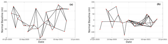
Figure 2.
The interferometric combination of Small Baseline network for Sentinel-1A/B (a) descending and (b) ascending tracks. The red circles and black lines represent SAR image acquisitions and interferometric pairs, respectively.
For both PS and SB processing, the 30 m resolution digital elevation model (DEM) of the Shuttle Radar Topography Mission (SRTM) was used to remove the topographic phase [39]. After flattening and removing the topographic phase, the overall wrapped differential phase of a resolution cell is expressed as follows:
where denotes the wrapping operator, is the LoS deformation phase term, indicates the atmospheric delay phase, is the phase caused by the orbit error, represents the residual topographic phase caused by the DEM error, and is the random noise phase. The final deformation phase can be estimated and extracted from other phase terms by iteratively filtering in the temporal-spatial domain. The detailed processing chain can be referred to [37,40,41].
The displacement velocities measured from the time series InSAR are along the radar LoS direction. As a result, the displacement calculated from time series InSAR is composed of vertical, north, and east displacement components that can be represented as [42,43,44,45,46]:
where is the incidence angle, is the heading angle of the satellite (positive clockwise from the north), , , and are the vertical, eastward, and northward displacement, respectively and is the displacement measured in the radar LoS direction. Ideally, measurements from at least three viewing geometries are available to resolve the 3D deformation.
A stable area over the Guanzhou power station was selected to conduct a cross-validation between the descending and ascending measurements. This power station is presumed to be relatively stable (i.e., no deformation) during the InSAR acquisition period. Both descending and ascending measurements were first projected into the vertical direction assuming no horizontal displacements, and the differences between the projected vertical displacements from both orbits were calculated.
3.2. Multi-Temporal Optical Image Analysis
In this study, two time series post-failure POT results were investigated using the post-failure image on 24 June 2020 as a significant reference image. By referencing the post-failure image of 24 June 2020, twenty-one pre-failure images from 3 January 2020 to 16 June 2020 were used to derive the first post-failure time series POT result before 24 June 2020. After 24 June 2020, the post-failure image acquired on 24 June 2020 was selected as the reference image, forty-three post-failure images from 26 July 2020 to 11 June 2021 were used as secondary images to generate the second time series POT results. Optical POT technique was applied to obtain the time series post-failure displacement over the Aniangzhai slope through the COSI-Corr software for measuring sub-pixel ground surface deformation based on the image correlation method [47].
Three layers of the raw POT result can be derived, including displacements in East/West and North/South directions, and the signal-to-noise ratio (SNR). Positive values in the East/West and North/South displacement layers indicate eastward and northward movement, respectively. Negative values represent displacements toward the west and south. The SNR value ranges from 0 to 1, with higher values associated to measurements of higher quality. The overall optical image processing included four steps: Optimal parameter searching, image correlation, filtering process, and mismatch correction, as shown in Figure 3.
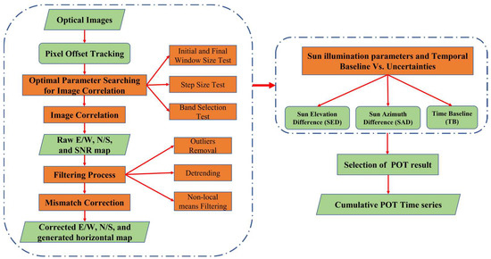
Figure 3.
Pixel offset tracking (POT) post-processing flowchart.
Image correlation in COSI-Corr requires determining several parameters, including the initial and final window sizes, the step size, and the band that would be used for input data of the pre-event and post-event images. This study conducted a sensitivity test to explore the relationship between these parameters and uncertainty. The optimal parameter searching for image correlation included three tests: Initial and final window size test, step size test, and band selection test. The final optimal combination of parameters was determined by investigating the relationship between the different combinations of parameters and the corresponding uncertainties (see Supplementary Material). This step led to the selection of an initial and final window size combination of 64-64 and a step size of 2 (Figures S1–S5). The red band of the PlanetScope images was used after the band selection test (Figures S6–S8). In terms of the filtering process, three major steps were included: (1) Outlier removal of pixels with SNR < 0.8 from the East/West and North/South displacement maps. A value of 0.8 was chosen as the SNR threshold since it can discard the correlation noise while keeping relatively higher spatial density of measurements over both displacement maps. (2) Removal of linear trend by fitting a polynomial surface to the stable area and then subtracting the surface from the generated results above [48]. (3) De-noising of maps was carried out using a non-local means filter [49]. To reduce the mismatch error of the displacement maps created after filtering, the displacements derived from the stable area were used to remove the residual co-registration faults. The mean East/West and North/South displacements derived from stable area were used to correct the image mismatch and generate the final corrected East/West and North/South displacement maps. The standard deviations of the East/West and North/South displacements in the stable area were used to justify the resulting uncertainties [50]. Then, the overall horizontal displacement was calculated based on the corrected East/West and North/South displacements.
The relationships between the differences in sun illumination parameters, temporal baseline of correlation pairs and the uncertainties were explored further. The differences in sun illumination parameters were defined as two major groups: Sun elevation difference (SED) and sun azimuth difference (SAD) between the correlated images. The sun elevation angle is the vertical angle between the sun and the local horizon, and the sun zenith angle is the angle between the sun and the local vertical vector. Therefore, the sun elevation angle of an optical image can be expressed as:
where is the sun elevation angle, and is the sun zenith angle. Therefore, the sun elevation difference between the optical image pair can be expressed as follows:
where and are the sun elevation angle for the reference and secondary images, respectively, in the used optical image pair. The sun azimuth angle is the angle of the sun’s rays measured in the horizontal plane from due south (true south) for the northern hemisphere or due north for the southern hemisphere. Then, the sun azimuth difference can be calculated as:
where and are the sun azimuth angle for the reference and secondary images, respectively, in the used optical image pair. Temporal baseline (TB) is the temporal separation between the acquisition time of the reference and secondary images, which can be written as:
where and are the acquisition date for the reference and secondary images, respectively, in the used optical image pair. Following a selection process, a threshold was set for these parameters, allowing for the POT results with considerable uncertainties to be discarded. The cumulative POT time series was created based on the selected POT results.
4. Results
4.1. Post-Failure Deformation Measured by Time Series InSAR Analysis
This research focuses on monitoring post-failure deformation through time series of InSAR to determine slope stability and provide information that is essential to risk assessment. The descending and ascending post-failure LoS deformation mean annual velocity maps were obtained (Figure 4). The measurement points with red colour (negative values) represent targets moving away from the satellite along the LoS direction, while those with blue colour represent motion toward the satellite. Our results show that the density of measurement points is relatively lower as the magnitude of displacement could exceed the upper limit that C-band data with the InSAR technique can measure.
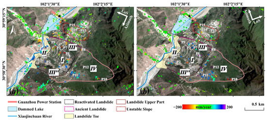
Figure 4.
Post-failure LoS deformation mean velocity detected from the Sentinel-1 (a) descending and (b) ascending datasets. The black star represents the reference point, and the black circles represent the selected measurement points.
The ANZ landslide is divided into four subzones (I–IV), and the post-failure deformation can be detected at four subzones from both the descending and ascending measurements. In zone (I), the maximum deformation velocity is −150 and 192 mm/year for the descending and ascending datasets, respectively. For zone (II), all the measurement points in the descending dataset were moving toward the satellite along the LoS direction (positive value), peaking at 196 mm/year near the Xiaojinchuan River. This could be due to the uplifted accumulation area at the toe caused by the sliding mess from the upper areas (zone I, III′, and IV). At zone (III′), 90% of the measurement points from the ascending datasets were positive, with a maximum LoS deformation velocity of up to 177 mm/year, as shown in Figure 4b. However, both positive and negative measurement points were observed from the descending datasets, peaking at 98 and −113 mm/year, respectively. Importantly, both datasets show a similar overall pattern of deformation at zone (IV). For example, the uplift movement (positive value) dominates in zone (IV), with the maximum LoS deformation velocity up to 105 and 186 mm/year for the descending and ascending measurements, respectively. Additionally, a small deformation mass in the upper section of zone (IV) was detected with negative value from both datasets, with the peak deformation velocity up to −55 and −111 mm/year for the descending and ascending measurements.
An unstable slope (located in the right side of the ANZ landslide detected from the pre-failure InSAR analysis by [10]), shows a maximum velocity of up to −52 and −30 mm/year for the descending and ascending measurements, respectively.
The results derived from the ascending and descending datasets were cross validated. A standard deviation of the differences of 4.6 mm/year is obtained between the projected vertical displacements from both orbits. The differences are mainly distributed in the range of −5 to 5 mm/year (Figure S9), accounting for about 70% of the measurement points, indicating that the two measurements are highly correlated with each other, and that the time series InSAR results are reliable.
To further explore the temporal evolution of the post-failure slope movement, the time series analysis of selected measurement points in both orbits are presented (Figure 5). Several measurement points located at four subzones of the ANZ landslide area were selected, as marked by the black circles in Figure 4. The monthly rainfall spanning from July 2020 to June 2021 was calculated from the daily rainfall based on the Climate Hazards Group InfraRed Precipitation with Station (CHIRPS) data from the Google Earth Engine [51,52]. At zone (I), the time series deformation of point P1 from the descending measurement initially showed a small acceleration under the action of heavy rainfall from July to September 2020, and then a linear deformation was observed for the whole dry season until an accelerated trend was detected since May 2021, as shown in Figure 5a. This was probably the response to the heavy rainfall in May 2021 of approximately 225 mm. At the same time, a similar change can be observed within the final two acquisitions at point P2 and P3 from the descending datasets. Changes in the final two acquisitions in P1 and P3 over the upstream part are more apparent than those of P2 over the downstream section. However, the ascending measurement at point P2 presented a relatively steady state with only a small fluctuation before December 2020. Point P3 exhibited a linear deformation during the whole observation period from the ascending dataset, and the accumulated LOS deformation is up to 160 mm.
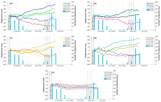
Figure 5.
Post-failure time series plotting for selected measurement points from the different zones. (a) Central (I) zone; (b) Toe (II) zone; (c) Upstream (III′) zone; (d) Upper slope (IV) zone; (e) Unstable slope in the post-failure mean velocity map (Figure 4). Note that the black dashed lines indicate the period of emergency engineering, and the grey dashed lines indicate the completion date of each activity in the on-going remediation engineering work.
Figure 5b depicts the time series deformation at zone (II), the landslide toe along the Xiaojinchuan River, demonstrating that the accumulated deformation at point P4 from both datasets and point P5 from the descending dataset fluctuated within a small range of about 30 mm before 2021, followed by a linear deformation trend until the end of the acquisition period. At point P6, a sharp fall was detected in the initial two acquisitions from the ascending dataset, with moving of about 32 mm between 7 July 2020 and 19 July 2020 when the peak monthly rainfall of 225 mm was recorded in July 2020. Until the end, it maintained a linear deformation trend. This is consistent with the detection of a sudden increase in deformation on 18 July 2020 from the field monitoring [7].
In terms of zone (III′) shown in Figure 5c, the upstream deformation zone, the time series deformation pattern is similar to zone (II). All three selected measurement points (P7, P8, and P9) from both datasets showed a relatively steady state until a linear deformation trend was observed since 2021. The declining measurement within the final two collections caused a noticeable decrease at position P7, lowering by around 23 mm in 12 days. This could be due to the severe rainfall in May 2021, which totalled about 225 mm. The accumulated LoS deformation was up to 124 mm at point P8 from the ascending datasets.
Over the landslide upper zone (IV), the time series deformation is shown in Figure 5d. At point P10, both measurements show a similar deformation trend, initially with a linear deformation trend with minor fluctuations, followed by a steady state since March 2021. At point P11, a linear trend was observed from both datasets for most of the period, while there was an evident change in deformation detected from the descending measurement in the last two acquisitions. At point P12, even with a slight fluctuation before October 2020, a linear deformation trend was observed until the end, with the accumulated LoS deformation up to 166 mm.
In terms of the unstable slope, time series analysis was also conducted based on three selected measurement points, as shown in Figure 5e. All the measurements points showed a relatively stable status during the observation period, and the accumulated LoS deformations ranged mainly between −50 and 50 mm. This demonstrated that the unstable slope discovered during the pre-failure stage had transformed to a stable state. Heavy rainfall throughout the rainy season is clearly found to impact deformation across the ANZ slope (from June to September). However, the local engineering work has clearly transformed the slope’s condition to linear deformation or stable state.
4.2. Time Series Post-Failure Displacements Detected from Optical Pixel Offset Tracking
Figure 6 shows the correlation results between the differences in sun illumination condition, temporal baseline, and uncertainties from East/West and North/South directions for all the post-processed POT results. Both the SED and SAD displayed a positive linear trend in both directions. However, SED showed a higher degree of correlation than SAD in both directions. The correlation coefficients for SED are 0.48 and 0.73 for the East/West and North/South directions, and 0.39 and 0.59 for SAD, respectively. It is worth noting that both the SED and SAD showed higher correlation coefficients in the North/South direction than those in the East/West direction. This could be due to the PlanetScope satellite’s orbit traveling North/South across the ANZ slope [53,54]. In terms of the relationship between the TB and uncertainty, both directions show a minor positive linear trend, although with significantly lower correlation coefficients, 0.13 and 0.11 in the East/West and North/South directions, respectively.
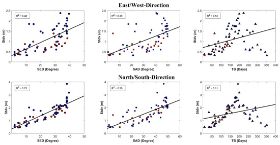
Figure 6.
Relationship between SED, SAD, TB, and uncertainties in the East/West direction (top) and North/South direction (bottom) for all the POT results. The red and blue colour indicate the first and second time series POT results, respectively. The circle, square, and triangle markers represent the SED, SAD, and TB, respectively. The black lines represent the best linear fits.
Based on the relationship between SED, SAD, TB, and uncertainties, it is found that the uncertainties in both directions are more sensitive to SED and SAD than TB and display a significant positive linear correlation. Therefore, all POT results were selected by limiting SED ≤ 10° and SAD ≤ 20° to control the uncertainties in both directions. Figure 7 shows the final cumulative POT time series with detailed information of the selected POT results in Table 2. The maximum uncertainties are only 0.61 and 0.88 m in the East/West and North/South directions, respectively, which are both less than one-third of the pixel resolution (3 m). In the first time series stage from 3 May 2020 to 16 June 2020, the horizontal displacements are detected at the middle and toe sections of the reactivated landslide area, especially the upstream part of these two sections, mainly ranging from 9.0 to 15.0 m. This could be owing to the outburst flood’s higher velocity and the consequent higher degree of erosion in the upstream area. It is worth noting that the deforming area over the upstream part of these two sections, mainly ranging from 12.0 to 15.0 m (light yellow patch in Figure 7), was gradually expanded as the temporal baseline was increased. However, there were no clear spatial coverage changes and magnitude in horizontal displacements over other areas. In terms of the second time series stage, the horizontal displacement over the upstream part of the middle section was increased up to the range of 12.0–15.0 m on 26 July 2020, where it was only in the range of 9.0–12.0 m on 16 June 2020 in the first time series stage. Then, the movements were continued in August 2020, rising to 15.0–18.0 m at the middle section. In 2021, it increased to 18.0–21.0 m over the middle section and remained relatively stable from May 2021 to June 2021. A deforming area ranging between 21 and 24 m, gradually expanding from 9 May 2021 to 11 June 2021 is observed over the top of the reactivated landslide area. Similarly, the upstream section of the ANZ landslide appears to be affected by the middle section with the cumulative displacements increasing from 3–6 m to 9–12 m between 26 July 2020 and 9 May 2021, subsequently stabilizing at this range until 11 June 2021. It is noted that the direction of horizontal displacement retrieved from the POT results is mainly the northwest direction, which agrees with the result from the field survey [6,8].
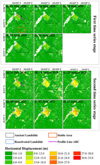
Figure 7.
Selected POT time series displacements from 3 May 2020 to 11 June 2021, including (a–e) on the top for the first time series stage (3 May 2020 to 16 June 2020) and (a–f) at the bottom for the second time series stage (26 July 2020 to 11 June 2021). Note that only the image pairs with limited sun illumination differences (SED ≤ 10° and SAD ≤ 20°) are used. Black arrows represent the directions of horizontal displacements.
Table 2.
Detailed information for the selected first and second time series POT results, including SED, SAD, TB, and uncertainties in the East/West and North/South.
The POT results were validated with the ground-based monitoring results from the published paper [7]. As shown in Figure 8, the spatial distribution of the horizontal displacements from the POT result is consistent with the ground displacements from the ground-based monitoring gauges. The ground-based displacements are slightly larger than the horizontal displacements from the POT result due to different temporal coverages (ground-based displacements from 22 June 2020 to 25 August 2020 versus horizontal displacements of POT result from 24 June 2020 to 25 June 2020). Moreover, the ground-based displacements include both horizontal and vertical displacements in this period. The maximum horizontal cumulative displacement from the ground-based measurements is up to 21 m, which is similar to the peak horizontal displacement from the POT result.
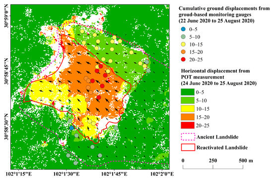
Figure 8.
Validation between ground-based monitoring result and the POT result. Note that the ground-based monitoring result is collected from the published paper [7]. Black arrows represent the directions of horizontal displacements.
5. Discussion
5.1. Factors Influencing POT Results
Sun illumination differences and temporal baseline between the reference and secondary image used for the image correlation significantly influence the generated POT results. Therefore, the relationship between these factors and uncertainties in the East/West and North/South directions was further investigated for all the generated POT results (see Figure 6). Although these three factors, including SED, SAD, TB, presented a positive linear trend in both directions, a higher degree of correlation can be found for the SED and SAD. After limiting these two factors (SED ≤ 10° and SAD ≤ 20°), the correlation coefficients of SED and SAD decreased to less than 0.45 in both directions (Figure 9). It is worth noting that SAD has a stronger correlation than SED in both directions, which could be related to the stricter constraints imposed on the SED. The TB presents a slight positive linear correlation with the uncertainties, with only 0.04 and 0.09 in the East/West and North/South directions, respectively.
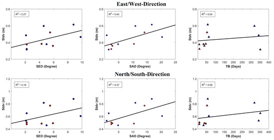
Figure 9.
Relationship between the SED, SAD, TB, and uncertainties in the East/West direction (top) and North/South direction (bottom) after imposing a limitation to SED and SAD (SED ≤ 10° and SAD ≤ 20°). The red and blue colour indicate the first and second time series POT results, respectively. The circle, square, and triangle markers represent the SED, SAD, and TB, respectively. The black lines represent the best linear fits.
To further explore the relationship between the differences in sun illumination conditions and uncertainties after applying equal limitations, both SED and SAD were restricted to less than 10°. As illustrated in Figure 10, both SED and SAD no longer exhibit a positive linear connection with uncertainty, and a distinct negative linear correlation can be seen in the North/South direction. Most importantly, an increasingly positive linear relationship between TB and uncertainties was clearly observed, especially in the North/South direction (a coefficient of up to 0.66). This result suggests that the TB becomes the most dominant factor influencing uncertainties in both directions when restricting the SED and SAD to less than 10°. Similar results have been reported by Ali et al. [53] using Landsat-8 and Sentinel-2 images for optical image correlation.
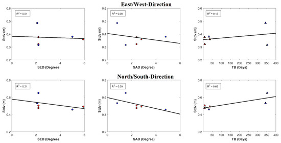
Figure 10.
Relationship between the SED, SAD, TB, and uncertainties in the East/West (top) and North/South (bottom) directions after imposing a limitation to SED and SAD (SED ≤ 10° and SAD ≤ 10°). The red and blue colour indicate the first and second time series POT results, respectively. The circle, square, and triangle markers represent the SED, SAD, and TB, respectively. The black lines represent the best linear fits.
This finding concurs with those of Lacroix et al. (2018) regarding uncertainties of POT results being controlled by restricting the temporal baseline of correlation images. In this study, a limitation of SED ≤ 10° and SAD ≤ 20° was applied to obtain the final POT time series result as more POT results with small uncertainties can be used under this selection process. Only six pairs resulted when restricting SED and SAD to less than 10°, while that grew to eleven pairs when SAD was set at less than 20°.
The results (Figure 6) also evidence that the relationship between TB and uncertainties initially presented an increasingly positive linear trend before 200 days, while a sudden drop of correlation occurs after that time. Further analysis of the relation between TB and uncertainties, by dividing all the POT pairs into four groups based on TB: 0 < TB ≤ 200 days, 200 < TB ≤ 360 days, 0 < TB ≤ 100 days, and 0 < TB ≤ 60 days (see Figure S10) shows that between the first two groups a high degree of positive linear correlation occurs when the TB is less than 200 days, while the relation becomes a negative linear when TB ranges between 200 and 365 days. This result suggests that TB would not support the POT results with smaller uncertainties, contrary to the finding of Lacroix et al. that the shorter TB reduces the uncertainties [20]. Therefore, only when applying a threshold to SED and SAD (e.g., SED ≤ 10° and SAD ≤ 10°), the uncertainties can be reduced by restricting the TB. If the TB is restricted to 100 and 60 days, only a slight positive linear correlation is observed between TB and uncertainties (i.e., a correlation coefficient lower than 0.2). When compared to a TB of less than 200 days, the positive linear correlations with SED and SAD drop when the maximum TB is set to 100 days, but improve significantly when the maximum TB is set to 60 days. It is worth noting that both SED and SAD present a higher degree of correlation with uncertainties than TB in these groups. When the TB is restricted (e.g., 100 and 60 days), the SED and SAD become the major factors controlling the uncertainties.
5.2. Post-Failure Temporal and Spatial Evolution of the ANZ Landslide
To further investigate the spatial evolution of the ANZ landslide, a profile line ABC along the upstream part of the middle section of the reactivated area was extracted for the first and second time series stage. The location of profile line II′ is shown in Figure 6. Figure 11 illustrates the horizontal displacements of various stages along the profile line ABC. In the first time series stage, the horizontal displacements over the lower slope (elevation between 2200 and 2500 m) range between 10 and 12 m, while this reduces to less than 3 m at the upper slope (elevation between 2500 and 2700 m). A similar trend of horizontal displacements is observed, with slight changes in horizontal displacements observed along the line, and less than 2 m in difference between 3 May 2020 and 16 June 2020. These results show a relatively low displacement rate over this time period, consistent with published results from the pre-failure InSAR time series analysis. No apparent acceleration was detected before 17 June 2020 [7,10].
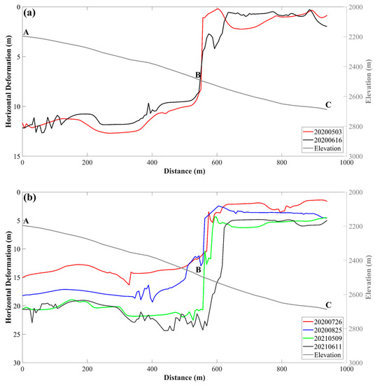
Figure 11.
Profile plot along the profile line ABC for the (a) first time series stage from 3 May 2020 to 16 June 2020 and (b) second time series stage from 26 July 2020 to 11 June 2021. The location of profile line ABC is indicated in Figure 7.
In terms of the evolution of the second time series stage, horizontal displacement increased by 3–5 m over the lower slope between 26 July 2020 and 25 August 2020 (within 1 month), with only 2 m rise over the upper slope. The period of 25 August 2020 to 9 May 2021 showed an increase between 2 and 8 m over the lower slope, with dramatic changes observed between 400 and 600 m along the profile line II′ where the head scarps are located. In 2021, the horizontal displacements increased between 19 and 24 m over the lower slope. When comparing the last two dates, it is evident that the horizontal displacements in 2021 tend to be stabilized over most sections of the line, except for the section across the head scarps. Apparent changes over the head scarps might be attributed to the high decorrelation caused by the large collapsed area. Similarly, minor changes with less than 1 m were observed over the upper slope, indicating that this area was stable in 2021. Changes in horizontal displacement are evident in the second time series, especially from July 2020 to August 2020. In this period, the ANZ landslide was still experiencing an acceleration status at the post-failure stage, as reported by field-based monitoring [7].
To explore the temporal evolution of horizontal displacements, time series analysis was also conducted over the selected measurement points from InSAR time series analysis based on the second time series POT results. The mean of the pixels in a specific spatial distance (with a radius of 50 m) was calculated. Figure 12 shows the POT time series analysis from the second time series stage (24 June 2020 and 11 June 2021), including nine selected points at four zones over the ANZ slope and the neighbouring unstable slope. A dramatic rise in horizontal displacements was observed for the points selected over the middle (P1, P2, and P3), toe (P6), and upstream (P7) sections of the reactivated ANZ landslide between 24 June 2020 and 26 July 2020, with the maximum horizontal displacement up to 14 m over the middle section. This is followed by a deceleration (between 27 July 2020 and 19 August 2020), which is consistent with field monitoring results [7,8]. This slowing down of deformation is likely related to the emergency engineering work by rechannelling the river position over the foot of the slope. Subsequently, P1, P3, and P7—along the upstream section show a linear trend. A slight acceleration is observed for P2 and P6, next to the downstream section, between 19 August 2020 and 25 August 2020. This could be caused by the high monthly rainfall of 140 mm in August 2020. During this period, the deformation rate over the downstream section outstrips the upstream section, indicating that the downstream section was gradually affected by the large displacements occurring in the upstream section, as seen in other studies [5]. Conversely, the upper shoulder section (P10, P11, and P12) shows an acceleration since 26 July 2020, followed by a sharp change in horizontal displacement for P11 between 19 August 2020 and 25 August 2020, and an ongoing linear trend for P10 and P12. It could be assumed that as the middle and lower sections moved by 8–14 m until 26 July 2020, the upper section gradually lost support, presenting an accelerated trend, characteristic of a retrogressive failure mode.
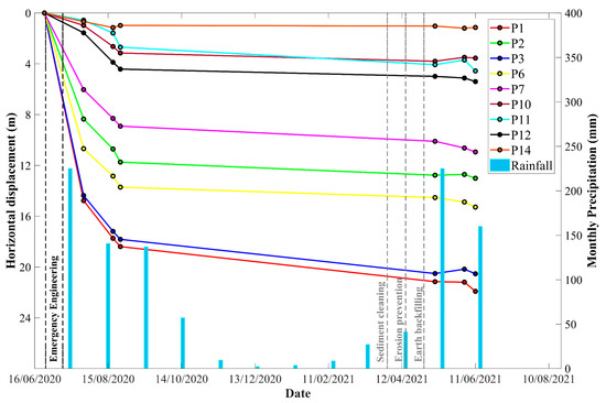
Figure 12.
Time series analysis of the selected points over the POT pairs from the second time series stage (26 July 2020 to 11 June 2021). The location of selected points is indicated in Figure 7. Central zone: P1–P3; Toe zone: P6; Upstream zone: P7; Upper slope zone: P10–P12; Unstable slope: P14. Note that the black dash lines indicate the period of emergency engineering, and the grey dash lines indicate the completion date of each activity in the on-going remediation engineering work.
Horizontal displacements of all points over the ANZ slope (P1–P12) slowed down significantly until May 2021 (less than 3 m observed within 8 months), concurrent with the linear trend status detected from the InSAR time series analysis in the same period. Both approaches demonstrate the success of preventive engineering work, and its effectiveness in reducing the risk of failure of the reactivated ANZ landslide. A slight increase in horizontal displacement is observed between 9 May 2021 and 11 June 2021 (less than 1 m within 1 month), which is consistent with the slight acceleration detected from the InSAR time series analysis between the 22 May 2021 and 3 June 2021. Increasing rainfall (starting from May 2021) could be a likely reason for this change. The deformations change was significantly smaller than the previous acceleration stage, indicating that this is a normal response to the rainfall season. Non-noticeable changes in horizontal displacements were detected for the neighbouring unstable slope for the whole observation period, suggesting that it has transitioned to a stable status, which is also consistent with the InSAR time series deformation over this area. According to the optical POT and InSAR time series analysis, even though there were several accelerations in land displacement in the first 2 months after reactivation, the landslide body was steadily slowing down likely due to a series of preventive engineering activities that reduced the likelihood of collapse. However, the response to the rainfall season caused a small deformation to change in May 2021, suggesting that installing a drainage system could further reduce the risk of future rainfall-induced failure.
InSAR time series analysis appears more sensitive to subtle change in the LoS deformations, especially the changes along the vertical direction, but it is not sensitive to the movement along the North/South direction, as concluded in previous research by Wright et al. (2004) due to the near-polar orbits of SAR satellites. In this regard, the POT time series analysis, with accuracy up to 1/10 or 1/5 of pixel resolution (about 0.3 to 0.6 m in this study) could be used to detect large changes in horizontal displacements. Therefore, these two approaches are complementary, and can be applied for detecting the spatial and temporal evolution of landslides.
6. Conclusions
In this study, the post-failure deformation characteristics, and spatial-temporal evolution after the reactivation of the ancient ANZ landslide (covering the time fame of the preventive engineering work in 2021) were investigated using time series InSAR analysis and optical POT technique.
The InSAR time series analysis over several sections of the slope showed that the deformation of the reactivated ANZ landslide was gradually slowing down, and it has transitioned into a steady deformation state. Most importantly, a slight acceleration was found between 22 May 2021 and 3 June 2021 from the descending measurement in response to the increased rainfall in May 2021. Moreover, the unstable slope detected from the pre-failure stage had changed to a stable status.
It is worth noting that the sun illumination parameter is the most significant factor to control the quality of POT result. The uncertainties in the North/South direction showed a higher degree of correlation with SED and SAD than in the East/West direction. However, when the differences in sun illumination parameters are restricted (SED ≤ 10° and SAD ≤ 10° in this case), the TB becomes to the most dominant factor influencing uncertainties in both directions. From the selected POT time series displacements map, it is clearly observed that the horizontal displacements over the upstream section of the middle part gradually expanded the scale to the top and downstream sections, with the magnitude increasing from 9–15 m to 21–24 m. Additionally, profile plot along the upstream part of the middle section captured evident changes in horizontal displacement from July 2020 to August 2020. In this period, the ANZ landslide was still experiencing an acceleration status at the post-failure stage. From the time series analysis of selected points of the POT results, a de-acceleration was captured between 26 July 2020 and 19 August 2020 over the lower slope, while a further acceleration was observed over the upper slope. Then, the landslide body remained at a steady deformation state until May 2021, a slight acceleration was detected from 9 May 2021 to 11 June 2021, which is consistent with the time series InSAR result. The joint analysis of optical POT result and time series InSAR result demonstrated that the preventive engineering work effectively slowed down the deformation of the reactivated ANZ landslide, but it still can be affected by the increased precipitation during the rainfall season. Therefore, a drainage system is suggested to set up over the slope to mitigate the occurrence of acceleration and the risk of failure in the future.
Our results evidence the high complementarity of time series InSAR technique and optical POT technique for effective and reliable landslide monitoring during the post-failure stage. A joint use of these approaches can detect surface deformations over the slope in multi-scale (subtle change from InSAR versus large displacements from POT) and multi-direction (LoS displacements in InSAR versus horizontal displacements in POT), which can provide more information of deformation characteristic and spatial-temporal evolution of landslides after the reactivation.
Supplementary Materials
The following supporting information can be downloaded at: https://www.mdpi.com/article/10.3390/rs15020369/s1, Figure S1: Means, standard deviations, and SNR (measurement quality) in the stable area of POT results derived from the PlanetScope image pair between 16 June 2020 and 24 June 2020 with different combinations of initial and final window sizes after filtering process. Note that fixed step size is 2 and the red band is used.; Figure S2: Corrected horizontal displacement mapped from the PlanetScope image pair between 16 June 2020 and 24 June 2020 using different window size combinations (Initial-Final) corresponding to Figure S1.; Figure S3. Comparison of horizontal displacements between 64-X and 128-X window size combinations; Figure S4. Means, standard deviations, and SNR (measurement quality) in the stable area of POT results derived from the PlanetScope image pair between 16 June 2020 and 24 June 2020 with different step sizes. Note that the fixed initial-final window sizes of 64-64 and red band was used.; Figure S5. Corrected horizontal displacement mapped from the PlanetScope image pair between 16 June 2020 and 24 June 2020 using different step sizes with the fixed initial-final window sizes of 64-64 and red band.; Figure S6. Means, standard deviations, and SNR (measurement quality) in the stable area of POT results derived from the PlanetScope image pair between 16 June 2020 and 24 June 2020 with blue, green, red, and NIR bands. Note the fixed initial-final window sizes of 64-64 and a step size of 2 was used. Figure S7. Corrected horizontal displacement mapped from the PlanetScope image pair between 16 June 2020 and 24 June 2020 using different Bands (blue, green, red, and NIR) with the fixed initial-final window sizes of 64-64 and step size of 2.; Figure S8. Horizontal displacement of the whole ancient landslide based on difference of orthophotos collected from the unmanned aerial vehicles (UAVs). (a) Horizontal displacement of the whole ancient landslide in the first month. (b) Horizontal displacement of zone II in the first month. (c) Horizontal displacement of the whole ancient landslide in the second and third months. (d) Local subsidence of zone I. Note that this figure is sourced from [13]; Figure S9. Cross validation based on the differences between the projected vertical displacements from the post-failure descending and ascending InSAR measurements.; Figure S10. Relationship between SED, SAD, TB, and uncertainties in the East/West direction and North/South direction after imposing limitations to TB (0 < TB ≤ 200 days, 200 < TB < 360 days, 0 < TB ≤ 100 days, and 0 < TB ≤ 60 days). The red and blue colour indicate the first and second time series POT results, respectively. The circle, square, and triangle markers represent the SED, SAD, and TB, respectively. The black lines represent the best linear fits.; Table S1: Optical images acquired by the PlanetScope satellite for this study.
Author Contributions
Conceptualization, J.K. and A.H.-M.N.; methodology, J.K. and A.H.-M.N.; validation, J.K. and A.H.-M.N.; formal analysis, J.K. and A.H.-M.N.; investigation, J.K.; resources, J.K., A.H.-M.N. and L.G.; data curation, J.K.; writing—original draft preparation, J.K.; writing—review and editing, J.K., A.H.-M.N., L.G., G.I.M. and S.R.C.; supervision, A.H.-M.N., L.G. and G.I.M.; project administration, A.H.-M.N. All authors have read and agreed to the published version of the manuscript.
Funding
This research was funded by the Program for Guangdong Introducing Innovative and Entrepreneurial Teams (2019ZT08L213), National Natural Science Foundation of China (grant number 42274016), and Natural Science Foundation of Guangdong Province (grant number 2021A1515011483).
Acknowledgments
The authors thank ESA for providing the Sentinel-1A/B data and the Planet Labs Company for providing the PlanetScope data under a research and education license.
Conflicts of Interest
The authors declare no conflict of interest.
References
- Cui, P.; Su, F.; Zou, Q.; Chen, N.; Zhang, Y. Risk assessment and disaster reduction strategies for mountainous and meteorological hazards in Tibetan Plateau. Chin. Sci. Bull. 2015, 60, 3067–3077. [Google Scholar]
- Li, H.-B.; Qi, S.-C.; Yang, X.-G.; Li, X.-W.; Zhou, J.-W. Geological survey and unstable rock block movement monitoring of a post-earthquake high rock slope using terrestrial laser scanning. Rock Mech. Rock Eng. 2020, 53, 4523–4537. [Google Scholar] [CrossRef]
- Chen, X.Q.; Cui, P.; Li, Y.; Zhao, W.Y. Emergency response to the Tangjiashan landslide-dammed lake resulting from the 2008 Wenchuan Earthquake, China. Landslides 2011, 8, 91–98. [Google Scholar] [CrossRef]
- Fan, X.; Tang, C.X.; Van Westen, C.J.; Alkema, D. Simulating dam-breach flood scenarios of the Tangjiashan landslide dam induced by the Wenchuan Earthquake. Nat. Hazards Earth Syst. Sci. 2012, 12, 3031–3044. [Google Scholar] [CrossRef]
- Szabó, J. The relationship between landslide activity and weather: Examples from Hungary. Nat. Hazards Earth Syst. Sci. 2003, 3, 43–52. [Google Scholar] [CrossRef]
- Zhao, B.; Zhang, H.; Hongjian, L.; Li, W.; Su, L.; He, W.; Zeng, L.; Qin, H.; Dhital, M.R. Emergency response to the reactivated Aniangzhai landslide resulting from a rainstorm-triggered debris flow, Sichuan Province, China. Landslides 2021, 18, 1115–1130. [Google Scholar] [CrossRef]
- Yan, Y.; Cui, Y.; Liu, D.; Tang, H.; Li, Y.; Tian, X.; Zhang, L.; Hu, S. Seismic signal characteristics and interpretation of the 2020 “6.17” Danba landslide dam failure hazard chain process. Landslides 2021, 18, 2175–2192. [Google Scholar] [CrossRef]
- Zhu, L.; He, S.; Qin, H.; He, W.; Zhang, H.; Zhang, Y.; Jian, J.; Li, J.; Su, P. Analyzing the multi-hazard chain induced by a debris flow in Xiaojinchuan River, Sichuan, China. Eng. Geol. 2021, 293, 106280. [Google Scholar] [CrossRef]
- Ning, L.; Hu, K.; Wang, Z.; Luo, H.; Qin, H.; Zhang, X.; Liu, S. Multi-hazard chain reaction initiated by the 2020 Meilong debris flow in the Dadu River, Southwest China. Front. Earth Sci. 2022, 321, 142. [Google Scholar] [CrossRef]
- Danba Media Center. Aniangzhai Landslide Remedial Engineering in Danba Country. 2021. Available online: https://www.163.com/dy/article/G5PFMU3T0550AS4X.html (accessed on 6 June 2022).
- Kuang, J.; Ng, A.H.-M.; Ge, L. Displacement Characterization and Spatial-Temporal Evolution of the 2020 Aniangzhai Landslide in Danba County Using Time-Series InSAR and Multi-Temporal Optical Dataset. Remote Sens. 2021, 14, 68. [Google Scholar] [CrossRef]
- Jiang, N.; Li, H.-B.; Hu, Y.-X.; Zhang, J.-Y.; Dai, W.; Li, C.-J.; Zhou, J.-W. Dynamic evolution mechanism and subsequent reactivated ancient landslide analyses of the “6.17” Danba sequential disasters. Bull. Eng. Geol. Environ. 2022, 81, 149. [Google Scholar] [CrossRef]
- Jiang, N.; Li, H.; Hu, Y.; Zhang, J.; Dai, W.; Li, C.; Zhou, J.-W. A Monitoring Method Integrating Terrestrial Laser Scanning and Unmanned Aerial Vehicles for Different Landslide Deformation Patterns. IEEE J. Sel. Top. Appl. Earth Obs. Remote Sens. 2021, 14, 10242–10255. [Google Scholar] [CrossRef]
- Simons, M.; Rosen, P. Interferometric synthetic aperture radar geodesy. Geodesy 2007, 3, 391–446. [Google Scholar]
- Dong, J.; Zhang, L.; Li, M.; Yu, Y.; Liao, M.; Gong, J.; Luo, H. Measuring precursory movements of the recent Xinmo landslide in Mao County, China with Sentinel-1 and ALOS-2 PALSAR-2 datasets. Landslides 2018, 15, 135–144. [Google Scholar] [CrossRef]
- Luo, S.; Feng, G.; Xiong, Z.; Wang, H.; Zhao, Y.; Li, K.; Deng, K.; Wang, Y. An Improved Method for Automatic Identification and Assessment of Potential Geohazards Based on MT-InSAR Measurements. Remote Sens. 2021, 13, 3490. [Google Scholar] [CrossRef]
- Dai, K.; Xu, Q.; Li, Z.; Tomás, R.; Fan, X.; Dong, X.; Li, W.; Zhou, Z.; Gou, J.; Ran, P. Post-disaster assessment of 2017 catastrophic Xinmo landslide (China) by spaceborne SAR interferometry. Landslides 2019, 16, 1189–1199. [Google Scholar] [CrossRef]
- Zhu, Y.; Qiu, H.; Liu, Z.; Wang, J.; Yang, D.; Pei, Y.; Ma, S.; Du, C.; Sun, H.; Wang, L. Detecting Long-Term Deformation of a Loess Landslide from the Phase and Amplitude of Satellite SAR Images: A Retrospective Analysis for the Closure of a Tunnel Event. Remote Sens. 2021, 13, 4841. [Google Scholar] [CrossRef]
- Raspini, F.; Ciampalini, A.; Del Conte, S.; Lombardi, L.; Nocentini, M.; Gigli, G.; Ferretti, A.; Casagli, N. Exploitation of amplitude and phase of satellite SAR images for landslide mapping: The case of Montescaglioso (South Italy). Remote Sens. 2015, 7, 14576–14596. [Google Scholar] [CrossRef]
- Delacourt, C.; Allemand, P.; Berthier, E.; Raucoules, D.; Casson, B.; Grandjean, P.; Pambrun, C.; Varel, E. Remote-sensing techniques for analysing landslide kinematics: A review. Bull. Société Géologique Fr. 2007, 178, 89–100. [Google Scholar] [CrossRef]
- Lacroix, P.; Bièvre, G.; Pathier, E.; Kniess, U.; Jongmans, D. Use of Sentinel-2 images for the detection of precursory motions before landslide failures. Remote Sens. Environ. 2018, 215, 507–516. [Google Scholar] [CrossRef]
- Yang, W.; Wang, Y.; Sun, S.; Wang, Y.; Ma, C. Using Sentinel-2 time series to detect slope movement before the Jinsha River landslide. Landslides 2019, 16, 1313–1324. [Google Scholar] [CrossRef]
- Ge, Y.; Tang, H.; Gong, X.; Zhao, B.; Lu, Y.; Chen, Y.; Lin, Z.; Chen, H.; Qiu, Y. Deformation monitoring of earth fissure hazards using terrestrial laser scanning. Sensors 2019, 19, 1463. [Google Scholar] [CrossRef]
- Pellicani, R.; Argentiero, I.; Manzari, P.; Spilotro, G.; Marzo, C.; Ermini, R.; Apollonio, C. UAV and airborne LiDAR data for interpreting kinematic evolution of landslide movements: The case study of the Montescaglioso landslide (Southern Italy). Geosciences 2019, 9, 248. [Google Scholar] [CrossRef]
- Wright, T.J.; Parsons, B.E.; Lu, Z. Toward mapping surface deformation in three dimensions using InSAR. Geophys. Res. Lett. 2004, 31, 169–178. [Google Scholar] [CrossRef]
- Du, Z.; Ge, L.; Ng, A.H.M.; Zhu, Q.; Yang, X.; Li, L. Correlating the subsidence pattern and land use in Bandung, Indonesia with both Sentinel-1/2 and ALOS-2 satellite images. Int. J. Appl. Earth Obs. Geoinf. 2018, 67, 54–68. [Google Scholar] [CrossRef]
- Samsonov, S.V.; d’Oreye, N. Multidimensional small baseline subset (MSBAS) for two-dimensional deformation analysis: Case study Mexico City. Can. J. Remote Sens. 2017, 43, 318–329. [Google Scholar] [CrossRef]
- Pepe, A.; Solaro, G.; Calo, F.; Dema, C. A minimum acceleration approach for the retrieval of multiplatform InSAR deformation time series. IEEE J. Sel. Top. Appl. Earth Obs. Remote Sens. 2016, 9, 3883–3898. [Google Scholar] [CrossRef]
- Liu, J.; Hu, J.; Xu, W.; Li, Z.; Zhu, J.; Ding, X.; Zhang, L. Complete Three-Dimensional Coseismic Deformation Field of the 2016 Central Tottori Earthquake by Integrating Left-and Right-Looking InSAR Observations With the Improved SM-VCE Method. J. Geophys. Res. Solid Earth 2019, 124, 12099–12115. [Google Scholar] [CrossRef]
- Morishita, Y.; Kobayashi, T.; Yarai, H. Three-dimensional deformation mapping of a dike intrusion event in Sakurajima in 2015 by exploiting the right-and left-looking ALOS-2 InSAR. Geophys. Res. Lett. 2016, 43, 4197–4204. [Google Scholar] [CrossRef]
- Ren, J.; Xu, X.; Zhang, S.; Yeats, R.S.; Chen, J.; Zhu, A.; Liu, S. Surface rupture of the 1933 M 7.5 Diexi earthquake in eastern Tibet: Implications for seismogenic tectonics. Geophys. J. Int. 2018, 212, 1627–1644. [Google Scholar] [CrossRef]
- Chen, X.; Zhou, Q.; Ran, H.; Dong, R. Earthquake-triggered landslides in southwest China. Nat. Hazards Earth Syst. Sci. 2012, 12, 351–363. [Google Scholar] [CrossRef]
- Ge, L.; Zhang, K.; Ng, A.; Dong, Y.; Chang, H.-C.; Rizos, C. Preliminary results of satellite radar differential interferometry for the co-seismic deformation of the 12 May 2008 Ms8. 0 Wenchuan earthquake. Geogr. Inf. Sci. 2008, 14, 12–19. [Google Scholar]
- Xia, Z.; Motagh, M.; Li, T.; Roessner, S. The June 2020 Aniangzhai landslide in Sichuan Province, Southwest China: Slope instability analysis from radar and optical satellite remote sensing data. Landslides 2022, 19, 313–329. [Google Scholar] [CrossRef]
- Ferretti, A.; Fumagalli, A.; Novali, F.; Prati, C.; Rocca, F.; Rucci, A. A new algorithm for processing interferometric data-stacks: SqueeSAR. IEEE Trans. Geosci. Remote Sens. 2011, 49, 3460–3470. [Google Scholar] [CrossRef]
- Hooper, A.; Segall, P.; Zebker, H. Persistent scatterer interferometric synthetic aperture radar for crustal deformation analysis, with application to Volcán Alcedo, Galápagos. J. Geophys. Res. Solid Earth 2007, 112, 1–21. [Google Scholar] [CrossRef]
- Hooper, A. A multi-temporal InSAR method incorporating both persistent scatterer and small baseline approaches. Geophys. Res. Lett. 2008, 35. [Google Scholar] [CrossRef]
- Fattahi, H.; Agram, P.; Simons, M. A network-based enhanced spectral diversity approach for TOPS time-series analysis. IEEE Trans. Geosci. Remote Sens. 2016, 55, 777–786. [Google Scholar] [CrossRef]
- Farr, T.G.; Rosen, P.A.; Caro, E.; Crippen, R.; Duren, R.; Hensley, S.; Kobrick, M.; Paller, M.; Rodriguez, E.; Roth, L.; et al. The shuttle radar topography mission. Rev. Geophys. 2007, 45, 1–33. [Google Scholar] [CrossRef]
- Hooper, A.; Zebker, H.A. Phase unwrapping in three dimensions with application to InSAR time series. JOSA J. Opt. Soc. Am. A 2007, 24, 2737–2747. [Google Scholar] [CrossRef]
- Bekaert, D.; Walters, R.; Wright, T.; Hooper, A.; Parker, D. Statistical comparison of InSAR tropospheric correction techniques. Remote Sens. Environ. 2015, 170, 40–47. [Google Scholar] [CrossRef]
- Fialko, Y.; Simons, M.; Agnew, D. The complete (3-D) surface displacement field in the epicentral area of the 1999 Mw7.1 Hector Mine earthquake, California, from space geodetic observations. Geophys. Res. Lett. 2001, 28, 3063–3066. [Google Scholar] [CrossRef]
- Ng, A.H.-M.; Ge, L.; Li, X.; Abidin, H.Z.; Andreas, H.; Zhang, K. Mapping land subsidence in Jakarta, Indonesia using persistent scatterer interferometry (PSI) technique with ALOS PALSAR. Int. J. Appl. Earth Obs. Geoinf. 2012, 18, 232–242. [Google Scholar] [CrossRef]
- Bayramov, E.; Buchroithner, M.; Kada, M.; Zhuniskenov, Y. Quantitative Assessment of Vertical and Horizontal Deformations Derived by 3D and 2D Decompositions of InSAR Line-of-Sight Measurements to Supplement Industry Surveillance Programs in the Tengiz Oilfield (Kazakhstan). Remote Sens. 2021, 13, 2579. [Google Scholar] [CrossRef]
- Xiong, L.; Xu, C.; Liu, Y.; Wen, Y.; Fang, J. 3D displacement field of Wenchuan Earthquake based on iterative least squares for virtual observation and GPS/InSAR observations. Remote Sens. 2020, 12, 977. [Google Scholar] [CrossRef]
- Fuhrmann, T.; Garthwaite, M.C. Resolving three-dimensional surface motion with InSAR: Constraints from multi-geometry data fusion. Remote Sens. 2019, 11, 241. [Google Scholar] [CrossRef]
- Leprince, S.; Ayoub, F.; Klinger, Y.; Avouac, J.P. Co-registration of optically sensed images and correlation (COSI-Corr): An operational methodology for ground deformation measurements. In Proceedings of the 2007 IEEE International Geoscience and Remote Sensing Symposium, Barcelona, Spain, 23–28 July 2007. [Google Scholar]
- Ayoub, F.; Leprince, S.; Keene, L. User’s Guide to COSI-CORR Co-Registration of Optically Sensed Images and Correlation; California Institute of Technology: Pasadena, CA, USA, 2009; Volume 38, p. 49s. [Google Scholar]
- Goossens, B.; Luong, H.; Pizurica, A.; Philips, W. An improved non-local denoising algorithm. In Proceedings of the 2008 International Workshop on Local and Non-Local Approximation in Image Processing (LNLA 2008), Lausanne, Switzerland, 23–24 August 2008. [Google Scholar]
- Yang, W.; Wang, Y.; Wang, Y.; Ma, C.; Ma, Y. Retrospective deformation of the Baige landslide using optical remote sensing images. Landslides 2020, 17, 659–668. [Google Scholar] [CrossRef]
- Funk, C.; Peterson, P.; Landsfeld, M.; Pedreros, D.; Verdin, J.; Shukla, S.; Husak, G.; Rowland, J.; Harrison, L.; Hoell, A.; et al. The climate hazards infrared precipitation with stations—A new environmental record for monitoring extremes. Sci. Data 2015, 2, 150066. [Google Scholar] [CrossRef] [PubMed]
- Banerjee, A.; Chen, R.; Meadows, M.E.; Singh, R.; Mal, S.; Sengupta, D. An analysis of long-term rainfall trends and variability in the uttarakhand himalaya using google earth engine. Remote Sens. 2020, 12, 709. [Google Scholar] [CrossRef]
- Ali, E.; Xu, W.; Ding, X. Improved optical image matching time series inversion approach for monitoring dune migration in North Sinai Sand Sea: Algorithm procedure, application, and validation. ISPRS J. Photogramm. Remote Sens. 2020, 164, 106–124. [Google Scholar] [CrossRef]
- Lacroix, P.; Araujo, G.; Hollingsworth, J.; Taipe, E. Self-Entrainment Motion of a Slow-Moving Landslide Inferred From Landsat-8 Time Series. J. Geophys. Res. Earth Surf. 2019, 124, 1201–1216. [Google Scholar] [CrossRef]
Disclaimer/Publisher’s Note: The statements, opinions and data contained in all publications are solely those of the individual author(s) and contributor(s) and not of MDPI and/or the editor(s). MDPI and/or the editor(s) disclaim responsibility for any injury to people or property resulting from any ideas, methods, instructions or products referred to in the content. |
© 2023 by the authors. Licensee MDPI, Basel, Switzerland. This article is an open access article distributed under the terms and conditions of the Creative Commons Attribution (CC BY) license (https://creativecommons.org/licenses/by/4.0/).