Abstract
Atmospheric fine particles () have been found to be harmful to the environment and human health. Recently, remote sensing technology and machine learning models have been used to monitor concentrations. Partial dependence plots (PDP) were used to explore the meteorology mechanisms between predictor variables and concentration in the “black box” models. However, there are two key shortcomings in the original PDP. (1) it calculates the marginal effect of feature(s) on the predicted outcome of a machine learning model, therefore some local effects might be hidden. (2) it requires that the feature(s) for which the partial dependence is computed are not correlated with other features, otherwise the estimated feature effect has a great bias. In this study, the original PDP’s shortcomings were analyzed. Results show the contradictory correlation between the temperature and the concentration that can be given by the original PDP. Furthermore, the spatiotemporal heterogeneity of -AOD relationship cannot be displayed well by the original PDP. The drawbacks of the original PDP make it unsuitable for exploring large-area feature effects. To resolve the above issue, multi-way PDP is recommended, which can characterize how the concentrations changed with the temporal and spatial variations of major meteorological factors in China.
1. Introduction
In recent years, due to the continuous increase in aerosols in developing countries, air pollution has become more serious [1,2]. (the particulate matter with aerodynamic equivalent diameter m) has become the main pollutant in the urban environment [3,4]. it contains a variety of toxic and harmful substances and can travel deeply into the lungs and increase the risk of multiple diseases [5]. Since is a serious threat to health, it should be monitored [6,7]. Understanding of causal and influential relation of concentration and the diverse variables helps to control fine particles and improve air quality. Many studies concern the -variable relationships and investigate these relations through their spatial distribution patterns [8,9]. Some previous researches analyze -meteorology relation via the temporal correlation [10,11]. However, the complicated interaction between concentrations and the influencing factors cannot be described well by linear correlation.
With the rapid development of remote sensing technology and machine learning methods, satellite-based aerosol optical depth and machine learning model has been widely used to estimate large areas and high-resolution concentrations [12]. These models can handle the complex nonlinear relationship between all predictor variables and concentration, so they can generate more accurate and detailed concentration distribution [13,14,15,16]. Based on such “black box” model with good performance, the previous studies try to explore the underlying mechanisms between predictor variables and concentration.
Among interpretable machine learning methods, partial dependence plot (PDP) [17] gets much attention for its superior performance. Previous studies use PDP to investigate the effects of individual features, including temperature, aerosol optical depth (AOD) and winds, on the predicted concentrations [18,19,20,21]. It can demonstrate the quantitative nonlinear relationships among variables. However, there are two key shortcomings to PDP: (1) it calculates the marginal effect of feature(s) have on the predicted outcome of a machine learning model, therefore some local effects might be hidden. A typical case is that surface winds substantially affect concentration, but the PDP shape of winds is almost a horizontal line [14]. The horizontal line means concentration does not vary with changes in winds, which is not the truth. However, because the increase [22] and reduce [23] effects of concentration could cancel each other out among regions in China. (2) it requires that the feature(s) for which the partial dependence is computed are not correlated with other features, otherwise the estimated feature effect has a great bias. When the independent assumptions are not satisfied, the PDP will create data points that do not exist in reality. This allows the PDP to give opposite interpretation results for the same feature.
In this study, the contradictory relationship between and temperature is drawn from the original PDP (hereinafter referred to as one-way PDP) and the spatiotemporal heterogeneity of -AOD relationship cannot be displayed well by one-way PDP. All results indicate there are uncertainties in the use and interpretation of one-way PDP and it is unsuitable for exploring large-area feature effects. To address the above shortcomings, the one-way PDP is expanded to multi-way PDP, which can reveal the regional and seasonal characteristics in the feature effects on concentrations quantitatively. Through embedded geospatial-temporal joint code (GTJC) [14], it can explore the multiple relationships between predictor variables and concentrations, i.e., the associations between meteorological factors, spatiotemporal factors and concentrations. With the visualization of multi-way PDP, variation details of concentration with temperature and AOD are analyzed and discussed. The results of this study suggest that multi-way PDP can give a relatively reliable relation between input features and model predictions.
2. Data
In order to better estimate concentrations, four kinds of variables are used as the input data of the model, i.e., satellite aerosol products, Human activity proxies, geographic factors and meteorological re-analysis data.
2.1. Station PM Observation
The hourly data are collected from the air quality monitoring network which is administrated by the China National Environment Monitoring Center (CNEMC, http://www.cnemc.cn/, accessed on 1 April 2022). The observation station network is shown in Figure 1a and a total of 1701 monitoring points are located in 367 cities in China. The Beijing-Tianjin-Hebei, Yangtze River Delta, Sichuan Basin, and Pearl River Delta are compared as representatives of urban agglomerations in different geographical contexts. observations obtained from air quality monitoring stations from 2015 to 2019 and processed into the daily average. The time series of daily average of all sites is shown in Figure 1b. The daily average data is matched to the grid cells of other features they fall in.
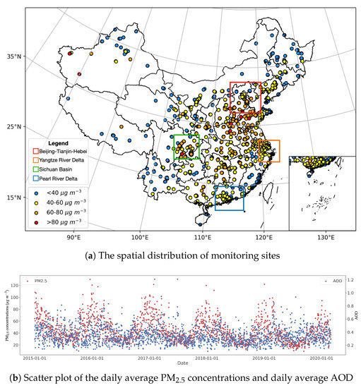
Figure 1.
(a) The spatial distribution of monitoring sites. The monitoring stations are illustrated as points and the color of the scattered point indicates the average of the concentration (g m) from 2015 to 2019. (b) Scatter plot of the daily average concentrations (g m) and daily average aerosol optical depth (AOD) of all observation sites from 2015 to 2019. The concentrations have notable seasonal variations, but the fluctuation of AOD is relatively flat.
2.2. Satellite Aerosol Products
The aerosol optical depth (AOD) is physically related to , since it measures the reduction effect of aerosol on the light in the entire atmospheric column [24]. Thus, the daily AOD products (MCD19A2) based on Multiangle Implementation of Atmospheric Correction (MAIAC) [25] are taken as main predictors in this study. It comes from Moderate Resolution Imaging Spectroradiometer (MODIS) and can be accessed at Distributed Active Archive Center (DAAC, https://lpdaac.usgs.gov/products/mcd19a2v006/, accessed on 1 April 2022). A comparison based on AErosol RObotic NETwork (AERONET) AOD shows that the retrieval accuracy of MAIAC AOD is higher than other common retrieval algorithms (MODIS Dark Target/Deep Blue) [26].
2.3. Human Activity Proxies
Human activity proxies include the land use cover (LUC) and nighttime light (NTL) products, which come from MODIS MCD12Q1v006 data [27] and the Suomi NPP VIIRS [28]. The distribution of urban and built-up Lands can be reflected from the land use parameters and the NTL products can provide population density information. So the emission sources caused by human activities can be inferred [29].
2.4. Geographic Factors
Geographic factors are used to describe the surface topography, including the digital elevation model (DEM) product and the normalized difference vegetation index (NDVI) data. The vegetation cover and terrain can be important influencing factors affecting the cross-regional transport of [12]. Thus, the Shuttle Radar Topography Mission (SRTM) DEM product [30] and the MODIS MOD13A3data [31] are collected to describe the transmission conditions.
2.5. Meteorological Re-Analysis Data
The variations of meteorological conditions can also affect the increase or decrease of concentration [32]. The ERA5 reanalysis products [33,34] provided hourly meteorological data. We collected 8 variables from it, including boundary layer height (BLH), 2 m temperature (TEM), 2 m dew point temperature (T), surface pressure (SP), total precipitation (PRE), evaporation (ET), 10 m U-components of wind (U) and 10 m V-components of wind (V). Combined with TEM, T and SP, the relative humidity (RH) values were calculated. The wind direction (WD) and wind speed (WS) are converted from the 10m U-components and 10m V-components of wind.
In order to build a more reliable model to explain, a more rigorous data cleaning was performed in this study. If a sample is missing any of the features, it will be removed from the dataset. The observations with an abnormal value of features will also be considered invalid samples. Table 1 summarizes the abnormal criteria and the statistics of collected features. The observation lasts for 12 h without change and will be considered an invalid observation. For extending the coverage of data, the each AOD of Terra and Aqua are averaged at every grid point. The hourly data of concentrations and meteorological data are averaged into daily values to match the time resolution of AOD data. The spatial resolution of all datasets is unified with AOD products by bilinear interpolation.

Table 1.
Statistics of collected features after data cleaning, including unit, range, mean, and standard deviation values.
3. Methodology
3.1. Overview
Figure 2 shows the workflow for exploring features- relation in this study. First, the relationship of and predictors is fitted by the gradient boosting decision tree (GBDT) model and geospatial-temporal joint codes (GTJC) model, respectively. Then, the built “black box” model is interpreted by permutation feature importances and partial dependence plots (PDP). The permutation feature importance is used to determine features of interest. The PDP can tell how concentrations change quantitatively with a certain amount of variation of selected features based on the built model. Finally, the interpretation results of the GBDT model and GTJC model are visualized and compared. The detail of each method will be separately described in the rest of this section.
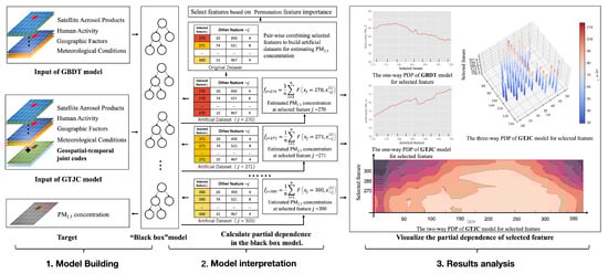
Figure 2.
The workflow for exploring features- relation, including model building, model interpretation and results analysis. Two models, geospatial-temporal joint codes (GTJC) and gradient boosting decision tree (GBDT) were built and interpreted by partial dependence plots (PDP). The calculation step of one-way PDP is illustrated in model interpretation. The interpretation results are visualized by multi-way PDP.
3.2. Model Building
3.2.1. Gradient Boosting Decision Tree Model
The gradient boosting decision tree (GBDT) [35] is a commonly used machine learning model for concentration estimation [36,37,38]. The results of GBDT are a combination of the output of weak learners. Each added weak learner will fit the residual between the target and the model output in the previous stage. In concentrations estimation, the input data of GBDT model include [, , , , , , , , , , , , ] and the target is concentrations.
3.2.2. Geospatial-Temporal Joint Codes Model
The relationship between concentrations and input data of GBDT, especially AOD, is spatial and temporal non-stationary [39]. The geospatial-temporal information is required by the model, otherwise the model would assume that all input data occurred at the same time and place. Therefore, geospatial-temporal joint codes (GTJC) [14] is applied to this study to help the model capture the spatiotemporal patterns. The day of the year (DOY), latitude () and longitude () of the given sample are converted to temporal codes (TC) and geospatial codes (GC) by a specific coding method, which has been described in Equation (1) and Figure 3.
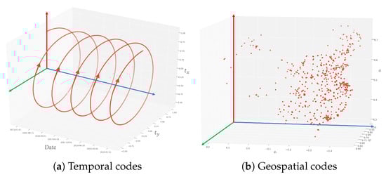
Figure 3.
Illustration of the (a) temporal codes (TC) and (b) geospatial codes (GC), which will be input as variables to the GTJC model.
Here, T is 365 or 366 and R is the radius of the Earth. R is set to 1 for normalization in the experiment. The day of the year (DOY) and the latitude () and longitude () of the given sample are converted into polar coordinates and spherical coordinates, respectively. TC and GC essentially are spatiotemporal information of the given sample in Cartesian coordinates; and and , and are the transformed coordinates.
The GTJC will be coupled with the observed data and this model is named the GTJC model. It should note that the difference between the GBDT model and the GTJC model is the absence or presence of GTJC as input.
3.2.3. Hyperparameter Selection
The model is built with scikit-learn [40]. Classification-and-regression-trees (CART) [41] is employed as the weak learner. concentration is estimated by CART through the following 5 steps: (1) Randomly sample 66% input data from the training data set for fitting the individual weak learners and randomly select 4 features for determining the best split; (2) The input data was assigned to two branches and based on a random split. This split was generated by selecting one arbitrary number a between the maximum and minimum of one feature A in step 1; (3) Calculate the squared error of and , where , is average of concentrations in and , respectively. Repeat step 2 to find the best feature A and split point a to minimize squared error; (4) Repeat step 2, 3 on and until the depth of the tree reaches 10; (5) The mean value of concentrations of input data in the leaf node will be taken as the estimated concentrations. The final model was constructed by 22,994 CART. The learning rate was set to 0.05 to shrink the contribution of each CART.
The most commonly used 10-fold cross-validation (10-CV) is adopted to evaluate the reasoning ability of the model [42,43,44]. For measuring the performance of regression, three quality metrics are used, i.e., determination coefficient (), mean absolute error (MAE), and root-mean-square error (RMSE).
3.3. Model Interpretation
3.3.1. Permutation Feature Importance
The feature importance can be measured by the decrease of the model score when this feature is randomly shuffled, which is also known as Permutation feature importance. In this study, the number of random shuffles is set to 10 times and the model score is measured by the mean squared error.
3.3.2. Partial Dependence Plots
The partial dependence plots (PDP) is a method for interpreting black-box models [45]. It is defined as
where x is the instances in the dataset and j is the j-th feature that we want to know the effect on the prediction . are other features of the black-box model F. E is mathematical expectation and P is probability. The partial function shows the relationship between j-th feature and the predicted targets.
The illustration of the calculation step of one-way PDP is shown in the model interpretation of Figure 2. First, the selected features are combined with other features one by one to build artificial datasets. Then, all artificial datasets are put into the ‘black box’ model to estimate concentrations. The average of estimated concentrations will be taken as the partial dependence of the corresponding feature. The partial dependence is estimated by marginalizing the predicted targets over the distribution of other features . Therefore, PDP can directly show how the prediction variates change with the input feature. However, as shown in Equation (2), the original PDP, i.e., one-way PDP, only shows the average marginal effects and lost some local effects. In order to show the hidden local effects and the detailed information, we expand PDP from one-way to multi-way. In the calculation of two-way PDP, the selected feature needs to be pair-wise combined with TC first, and then continue to follow the calculation steps of one-way PDP. Finally, to better understand the feature effects of the selected feature, we trace back to corresponding the day of year and visualize the partial dependence results. For three-way PDP, the selected feature is combined with geospatial codes.
4. Results
This section presents the results of both the model performance and interpretation methods. Section 4.1 shows the model performance. The relative importance of the feature is demonstrated in Section 4.2. Section 4.3 investigates TEM- concentrations relationship through comparing the one-way PDP of gradient boosting decision tree (GBDT) model and geospatial-temporal joint code (GTJC) model and its annual variation presented in the two-way PDP. Section 4.4 reveals the impacts of water vapor on the AOD- concentrations relationship via analysis of seasonal, regional and multi-way PDPs.
4.1. Model Performance
The results of sample-based 10-fold cross-validation are displayed in Table 2. The value of gradient boosting decision tree without geospatial-temporal joint code (GTJC) is 0.82. The value is increased to 0.85 after incorporating the spatial information. However, with the aid of the temporal information, is increased to 0.86. Compared with the general gradient boosting decision tree model, the GTJC improves the prediction performance in terms of both predictive quality and estimated uncertainty. The of the GTJC model is 0.89. This result indicates that concentrations observed by sites across China could be well explained by a combination of satellite-based aerosol products, geographic factors, human activity, surface meteorological conditions, time variables and space variables in the GTJC model.
Table 2.
The mean and variance of sample-based 10-fold cross-validation results of gradient boosting decision tree (GBDT), GBDT with geospatial codes, GBDT with temporal codes, and GBDT with geospatial-temporal joint codes.
4.2. Relative Importance of Features
Variables with a larger value of permutation feature importance have a greater influence on the model. Figure 4a,b shows the permutation feature importance of the GTJC model and GBDT model separately.
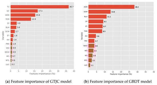
Figure 4.
Permutation feature importances of (a) geospatial-temporal joint codes model (GTJC) model and (b) gradient boosting decision tree (GBDT) model. The calculated feature importance values are normalized to percentages and sorted in descending order of importance.
In the GTJC model, the temporal codes (TC) and geospatial codes (GC) are the two most important features, whose importance values are 36.77% and 17.17%, respectively. This is consistent with previous studies that concentrations vary drastically over time and space [46,47,48], therefore, the estimation of concentrations across entire China is highly depending on geospatial location and time period. Generally, in winter, weather conditions are not in favor of the pollutants diffusion that can elevate the concentrations [49,50]. The emission amount is larger in northern China than in southern China due to the distribution of industry and indoor heating [51,52]. These synchronously changing in pollution emission, weather conditions and concentrations make TC and GC the most important factors in estimating concentrations. Besides the temporal and geospatial codes, the top-4 important features also include aerosol optical depth (AOD), and temperature (TEM). Other features have less contribution to the model, with an importance lower than 10%.
In the GBDT model, the importance value of AOD is 28.2%, which is much greater than that of other variables. This is because AOD is the total extinction of particulate matter in the entire atmospheric column, thus physically connected with concentration. The other input variables are the influencing factors of concentration. There, the contribution of AOD to concentration estimation is much greater than other factors. It is worth noting that the values of AOD do not discriminate the extinction for fine and coarse particles. Moreover, AOD is for the whole atmosphere column, but concentration is measured at the surface. Therefore, the AOD value does not strictly correspond to changes in concentrations. This inconsistency can be shown in Figure 1b, which may partially explain why the feature importance of AOD is falling lower than that of geospatial-temporal joint codes. The other features with an importance value over 10 % are DEM and BLH. In China, the altitude in the eastern plains is low and there will be more human activities here. Thus, the concentration there is usually high. On the Tibet Plateau in the west of China, the altitude is highest and the concentration is the lowest [53]. The -meteorology interactions are closely related to the variation in boundary layer height, which determines the vertical structure and diffusion height of . There is very little space for dispersion of if the BLH is small. This results in a higher concentration with the same amount of aerosol particles [54,55,56].
4.3. TEM-PM Concentrations Relationship Revealed by Multi-Way PDP
The entire China, the Beijing-Tianjin-Hebei, the Yangtze River Delta region, the Sichuan Basin, and the Pearl River Delta region were selected as study areas to analyze the relationship between and temperature (TEM). Figure 5 present the density scatterplots of TEM and observed of those regions. In each subfigure, statistical results are attached with the linear regression relation, the number of samples (N), the Pearson correlation coefficient (Pearson’s r). In our dataset, the Pearson’s r calculated for these five regions are all negative. The slopes of linear regressions are also negative.
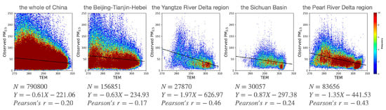
Figure 5.
The density scatterplots of temperature (TEM) and observed in the whole of China, the Beijing-Tianjin-Hebei, the Yangtze River Delta region, the Sichuan Basin and the Pearl River Delta region. In each subfigure, statistical results are attached with the linear regression relation, the number of samples (N), the Pearson correlation coefficient (Pearson’s r).
Figure 6 shows one-way PDP of TEM of the GBDT model and GTJC model across China. The PDP of GTJC model over mainland China is similar to that over the four regions, except for the difference in the range of estimated PM concentrations. All these PDPs of GTJC show that the estimated concentrations increased with the rising temperature. On the contrary, one-way PDPs of the GBDT model suggest that there is an inverse relationship between TEM and concentrations. The negative TEM- relation given by the one-way PDP of the GBDT model is more consistent with the TEM- relation demonstrated by the observed dataset in Figure 5.

Figure 6.
The one-way partial dependence plots (PDP) of temperature (TEM) of GBDT model and GTJC model. The black bars on the axes show the deciles of the feature values in the training data.
As stated in Section 3.2.2 that the difference between the GBDT model and the GTJC model is the absence or presence of GTJC as input. Therefore, the GTJC is speculated to be the reason for this discrepancy. The relation between TEM and concentrations in the one-way PDPs is almost the same among the four regions and mainland China for model with and without GTJC, respectively, suggesting the false relation is irrelevant to geospatial codes and induced by temporal codes. The contradictory relationship given by the one-way PDP will be analyzed and discussed in Section 5.1.
To further explore the relationship between TC, TEM, , we expand PDP to two-way to show how this relation variates with the day of the year. Two-way PDP in Figure 7a displays the joint dependence of estimated concentrations on both TC and TEM. Figure 7b,c presents the average of TEM and observed concentrations every month, respectively.
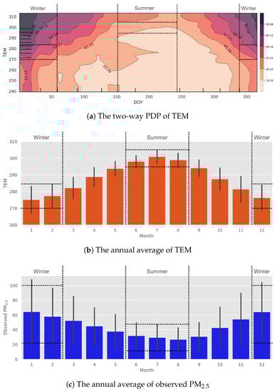
Figure 7.
(a) The two-way partial dependence plots (PDP) of temperature (TEM) for the GTJC model. The contour lines represent the average estimated concentrations (g m). The black bars on the axes show the deciles of the feature values in the training data. (b) Mean values of the TEM at a monthly scale. (c) Mean values of the concentrations at a monthly scale. The error bar referred to the standard deviation of the data set.
As shown in Figure 7b, the temperature is high in summer and low in winter. In the winter (i.e., December, January, and February.), the TEM is mainly distributed from 270 to 285 K. In the summer (i.e., June, July, August), the TEM reached 295 to 305 K. In Figure 7a, when the TEM is between about 270 and 285 K, the estimated concentration range is from 45.25 to 81.12 g m. In the summer, when the TEM reached to the range between 295 and 305 K, and the estimated concentration changes from 33.29 to 45.25 g m. The seasonal variation in TEM and estimated are diametrically opposed. Therefore, estimated concentrations are inversely related with TEM in the annual cycle, i.e., lighter pollution (higher TEM) in summer and heavier pollution (lower TEM) in winter. In Figure 7c, the observed ranges from 22 to 100 g m in winter and 10 to 50 g m in summer. Similarly, the variation of observed concentration is contrary to the variation of TEM. There is a negative correlation between observed and TEM. This result is consistent with that of estimated concentrations. It should be noted that the in Figure 7a is estimated by marginalizing the predicted targets over the distribution of unselected features. It will be different from the observed concentration.
TEM in most regions of mainland China has a distinct annual cycle with hot summer and cold winter due to its location in the northern temperate zone. Simultaneously, concentrations in summer stay at a low level because of the rainy weather and less emission compared with the heating season. This coincidentally seasonal variation in both TEM and concentrations makes them have a natural inverse relationship on the yearly scale. The negative TEM- concentrations relation is reflected by the one-way PDP of GBDT model in Figure 6.
4.4. AOD-PM Concentration Relationship Revealed by Multi-Way PDP
As shown in Figure 8a,b, the one-way PDPs in different seasons and two-way PDP shows seasonal changes of the AOD- relationship. For the same AOD value, the corresponding concentration value varies greatly from winter to summer. A more reliable AOD- concentration relationship for the individual region is revealed. However, two-way PDP can visualize annual variations in concentrations more detailed and intuitively with the changes in AOD across China.
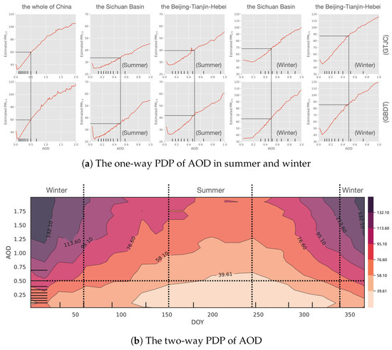
Figure 8.
(a) The one-way partial dependence plots (PDP) of aerosol optical depth (AOD) in the Beijing-Tianjin-Hebei and the Sichuan Basin during summer and winter. The dotted line represents the estimated concentration when AOD is 0.5. (b) The two-way PDP of AOD. The contour lines on the subfigure (b) represent the average estimated concentrations (g m). The black bars on the axes show the deciles of the feature values in the training data.
The AOD- concentration relation in one-way PDPs are all positive for the whole China, the Beijing-Tianjin-Hebei and the Sichuan Basin in both summer and winter, regardless of whether there is a GTJC in the model. Note that different from the relation of TEM- concentrations, concentrations are physically relative to AOD values. The positive correlation of TEM- concentrations within the season is not the direct relationship, but the regulated expression of the strengthened photochemical reaction and secondary pollutants formation under higher environment temperature. However, concentration dose positively related to AOD because they are quantities representing aerosol loading in the atmosphere.
As the columnar integration of the extinction coefficient with altitude, satellite AOD is affected by the atmospheric humidity since the uptake of water vapor can cause a substantial increase of aerosol size and its extinction. Whilst is often measured under a dry condition and less affected by the atmospheric humidity. Therefore, atmospheric humidity difference may result in changes in AOD- relationship. Figure 9a shows the probability density of relative humidity (RH) in Sichuan Basin and the Beijing-Tianjin-Hebei during winter and summer. As we can see, there is a huge contrast in humidity between the Sichuan Basin and the Beijing-Tianjin-Hebei. In winter, the RH in the Sichuan basin is mainly distributed in 60 to 80% and it is 20 to 50% in the Beijing-Tianjin-Hebei.
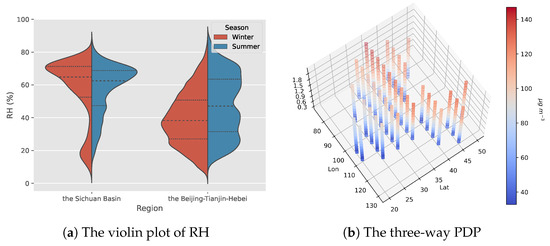
Figure 9.
(a) The violin plot of relative humidity (RH). The dotted line on (a) represents the quartiles of the RH distribution. (b) The three-way PDP of geospatial codes (GC) with respect to AOD. The latitude and longitude are inversely transformed from GC. The vertical axis of the three-way PDP is the selected feature, and the color represents the average estimated concentration (g m).
With the distinct humidity contrast, the one-way PDP of both the GTJC model and the GBDT model for the Sichuan Basin in winter is markedly different from that of the Beijing-Tianjin-Hebei in winter. The deciles of AOD indicated that the AOD of Sichuan Basin (0.3 to 0.9) is greater than that of the Beijing-Tianjin-Hebei (0.1 to 0.7) in winter but the variation range is smaller for concentrations over the Sichuan Basin in winter than that of the Beijing-Tianjin-Hebei in winter. In GTJC model, the concentrations vary from 50 g m to 100 g m in the Sichuan Basin, which is smaller than that of Beijing-Tianjin-Hebei (45 to 115 g m). In GBDT model, the variation range for concentrations of the Sichuan Basin is 35 to 110 g m and it is 40 to 120 g m. The flatter of one-way PDP means the variation of AOD results in weaker changes in the estimated concentrations. The larger AOD in winter is not necessarily due to the high concentration of , but due to the increased extinction effect by the hygroscopic of particles in higher environmental humidity. This is in line with the situation that in the Sichuan Basin during humid winter, changes in AOD may be more closely related to changes in water vapor rather than variations in concentrations. Both the GBDT and GTJC models can distinguish the impacts of water vapor on -AOD relation.
The joint dependence of concentrations on geographical codes and AOD is presented with three-way PDP in Figure 9b. According to Figure 9b, the sensitivity of estimated concentrations to AOD is higher in the north than that in the south of China. This agrees well with the one-way PDPs in Figure 8a that the corresponding increase of concentration of a certain variation in AOD is smaller in South China than that in North China. As analyzed above, the prime reason for this South–North contrast is that the higher atmospheric water vapors in South China swell the AOD value by hygroscopic growth of particles. Similarly, the East–West difference of the sensitivity of concentrations to AOD in the three-way PDP is also mainly originated from the atmospheric humidity difference between East and West regions in China. In addition, the higher fraction of cloud cover may introduce a large uncertainty into the AOD retrieval [57], leading to the less sensitivity of estimated concentration to AOD variation over southern China.
5. Discussion
5.1. The Contradictory Relationship Shown in the One-Way PDP
As stated in Section 4.3, for the same feature, temperature, the one-way PDP will give two opposed results since temporal codes. Here, Temporal codes are essentially spatiotemporal information of the given sample in Cartesian coordinates and , are the transformed coordinates. The daily average of concentrations, TEM, and are shown in Figure 10. The concentrations have notable seasonal variations, with the heaviest pollution in winter. The annual cycle is also substantial in TEM, but with the lowest values of TEM in winter. The Pearson correlation coefficient of and TEM is −0.17. Clearly, concentrations are negatively correlated with TEM from the perspective of annual changes. The variation of TC, represented by and , has a very similar annual cycle to that of concentrations. The Pearson correlation coefficients between and , are 0.34, 0.08, respectively. For better describe the relationship among TC, TEM, and , we claim that TC is positively correlated with even if TC consists of two elements. The Pearson correlation coefficients between TEM and , are −0.78 −0.15, respectively. It should be noted that TEM is physically determined by the seasonal changed solar radiation. Therefore, the two input variables of TEM and TC are naturally strongly correlated with each other.
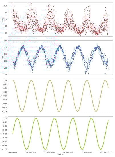
Figure 10.
Scatter plot of the daily average concentrations (g m), temperature (TEM), and of all observation sites from 2015 to 2019.
As shown in Figure 2, TEM are combined with TC one by one to build artificial datasets for estimating partial dependence. Based on the strong negative correlation of TEM and TC, a paired combination is not suitable for these two features. Therefore, some data points that do not exist in reality will be created, for example, extremely cold temperatures occur in the summer. These data points will be involved in the estimation of the average of concentrations.
For the complicated interactions between different factors, the extracted correlation coefficient between two variables could be influenced significantly by other variables in the ecosystem. In addition, correlation analysis between two variables in a complicated ecosystem might lead to mirage correlations [58]. Similarly, it is unreliable to analyze complex patterns learned by a “black box” model from the perspective of a feature, especially when the selected feature has a strong correlation with other predictors.
The coincidentally seasonal variation in TEM, and TC cause a strong correlation among them. However, the one-way PDP can only reveal the relationship between and a single feature. Furthermore, as shown in Figure 4a, TC has more influence on the model compared to TEM. Thus, the relationship between TEM and given by one-way PDP can be very partial. Actually, Christoph Molnar [45] indicates that the correlated features would complicate the partial dependence analysis. The results in this study further suggests the effect of the powerful feature with the output seems to cover up that of less influential feature with the output.
Note that within a certain period, such as a time scale of months, seasons, etc., concentrations increase with the increase of TEM, according to the two-way PDP in Figure 7a. The possible explanations are that more precursors of particles and secondary pollutants are generated under high temperatures, since it promotes the photochemical reaction in the atmosphere. Thereby resulting in the rise in concentrations within the corresponding period [32].
5.2. The Single Perspective of One-Way PDP
The one-way PDP can only demonstrate the relationship between a single predictor and target. In addition, the partial dependence is estimated by marginalizing the predicted target over the distribution of unselected features, as shown in Equation (2). Therefore some local effects might be hidden and quantifying the relationship from one-way PDP may deviate from the actual local situation.
For example, the dotted line in Figure 8a,b represents the estimated concentration when AOD is 0.5. It is 60 g m in the whole of China both in the GTJC model and GBDT model when AOD is 0.5. However, in summer, the estimated concentration of the GTJC model and GBDT model both is around 35 g m in Sichuan Basin and 40 g m in the Beijing-Tianjin-Hebei. Those results in summer are lower than the national average concentration. Meanwhile, in the winter, the estimated concentration of the GTJC model and GBDT model both reached 65 g in Sichuan Basin and 85 g m in the Beijing-Tianjin-Hebei. The concentrations estimated in winter are higher than the national average. In terms of regions, the estimated concentration also have slight differences.
These sub-regional and sub-seasonal results indicate that the -AOD relationship has spatiotemporal heterogeneity. The heterogeneous interactions might be hidden because one-way PDP can only quantify the influence of individual factors in an average state. However, the expanded multi-way partial dependence plots can visualize spatiotemporal variations of concentrations more detailed and intuitively with the changes in selected factors across China. As mentioned above, the drawbacks of the original one-way PDP make it unsuitable for exploring large-area feature effect. To reveal the spatiotemporal characteristics of feature effect, it is recommended to visualize the joint dependence in the form of multi-way PDP.
5.3. The Effect of Incorporating Spatial and Temporal Terms
The spatial and temporal variables are widely incorporated into concentrations estimation models because they can address the spatiotemporal heterogeneities of the -AOD relationship [12]. The common forms of spatial and temporal terms include the days of year [59], Unix Epoch time [21,60], Haversine [15], two-dimension smooth term of geographical coordinate [61]. The geospatial-temporal joint codes [14] used in this study is also one of the forms spatiotemporal variables. However, not all spatiotemporal variables will affect the results of one-way PDP.
The time variable, days of the year, is converted into a cycle with a range of [0, 2] in this study to solve the problem of the time variable jumping from 365/366 on the last day of a year to 1 on the first day of the next year. This conversion enables the time variable variates seasonally, resulting in the strong correlation among TC, temperature and concentrations. Other concentration prediction models with temporal codes but in the form of Unix Epoch time (number of seconds since 1 January 1970) get negative TEM-PM concentrations relationship [21,60], verifying the above suppose that it is the strong correlation between TC and temperature rather than TC itself that makes the model get different TEM- concentrations relation.
Spatiotemporal variables can also make the one-way PDP more reliable in the case of sparse data points. As shown in Figure 8a, in the summer of the Sichuan basin, AOD is mainly distributed in the range of 0.1 to 0.6. It almost has no data points between 0.6 and 1.0. The estimated concentrations of the GBDT model changed by more than 15 g m when AOD changed from 0.1 to 0.6 and it is 8 g m in GTJC model. This is where the two models’ one-way PDP differ most. When the distribution of data points is sparse, the spatiotemporal variables can offer additional information to the model’s decision. This is also why GTJC can improve the model’s ability.
6. Conclusions
The success of the machine learning model in estimating concentrations from satellite remote sensing data has led to the pursuit of interpretability. Due to the high spatiotemporal heterogeneity, understanding the relationship between predictors and concentration remains challenging. To obtain a more reliable relation of temperature (TEM) and AOD with concentrations, partial dependence plots (PDP) and their extended forms are used to thoroughly explore the relationship of the prediction and input features in the machine learning model.
Temperature is found to be inversely correlated with concentration in the one-way PDP of the model without geospatial-temporal joint codes (GTJC) and in the annual scale of the two-way PDP with GTJC. The comparison of one-way PDPs between the model with and without GTJC suggests that the strong correlations of temporal codes with concentration and TEM lead to an artificial positive TEM- concentration relation. Future studies need to use one-way PDP with caution because it is susceptible when the input variables have a correlation. As recommended in this study, the extension of PDP from one-way to two-way can clarify to some degree of the TEM- concentration relation by visualizing its annual evolution.
For AOD- concentration relation, If we analyze the one-way PDP of the whole of China, the distinct regional and seasonal characters would be hidden. From the perspective of obtaining empirical and numerical relationships, one-way PDP is not suitable for exploring AOD- concentration relation over large-scale regions of high inhomogeneous. Therefore, we combine GTJC with the model and thus expand PDP to two-way and three-way to dive into the details of seasonal and regional variations.
This study let us dive into the spatial and temporal characters of the relationship of AOD, TEM and concentration. The results suggest that multi-way PDP can give a relatively reliable relation between input features and model predictions than one-way PDP. This further illustrates the important role of GTJC-based multi-way PDP in the analysis of individual factor- concentration relationship. Therefore, it is recommended to use multi-way PDP to explain the “black box” model. In the future, the dependence of concentrations on interactions between meteorological factors is interesting and needs to be further analyzed. It will contribute to the improvement of climate prediction with better understanding of concentrations–multifactor relationship.
Author Contributions
Conceptualization, H.T. and X.Y.; methodology, H.S. and N.Y.; software, H.S. and N.Y.; validation, H.S., N.Y. and H.T.; formal analysis, H.T.; investigation, H.S.; resources, X.Y.; data curation, H.S.; writing—original draft preparation, H.S.; writing—review and editing, H.T., N.Y. and X.Y.; visualization, H.S.; supervision, H.T. and X.Y.; project administration, X.Y.; funding acquisition, X.Y. All authors have read and agreed to the published version of the manuscript.
Funding
This work was supported by the National Natural Science Foundation of China under Grant 42271332 and 41971280.
Data Availability Statement
Publicly available datasets were analyzed in this study. The hourly data are collected from the China National Environment Monitoring Center (CNEMC, http://www.cnemc.cn/, accessed on 1 April 2022). The Moderate Resolution Imaging Spectroradiometer (MODIS) data can be accessed at Distributed Active Archive Center (DAAC, https://lpdaac.usgs.gov/products/mcd19a2v006/, accessed on 1 April 2022). The nighttime light (NTL) products come from the Suomi NPP VIIRS (https://ncc.nesdis.noaa.gov/VIIRS/, accessed on 1 April 2022) The Shuttle Radar Topography Mission (SRTM) DEM product are available online (http://srtm.csi.cgiar.org/, accessed on 1 April 2022). The ERA5 were available from the Copernicus Climate Change Service (C3S) Climate Data Store (CDS) (https://cds.climate.copernicus.eu/, accessed on 1 April 2022).
Conflicts of Interest
The authors declare no conflict of interest.
References
- Pant, P.; Harrison, R.M. Estimation of the contribution of road traffic emissions to particulate matter concentrations from field measurements: A review. Atmos. Environ. 2013, 77, 78–97. [Google Scholar] [CrossRef]
- Van Donkelaar, A.; Martin, R.V.; Brauer, M.; Hsu, N.C.; Kahn, R.A.; Levy, R.C.; Lyapustin, A.; Sayer, A.M.; Winker, D.M. Global estimates of fine particulate matter using a combined geophysical-statistical method with information from satellites, models, and monitors. Environ. Sci. Technol. 2016, 50, 3762–3772. [Google Scholar] [CrossRef]
- Sun, L.; Wei, J.; Duan, D.; Guo, Y.; Yang, D.; Jia, C.; Mi, X. Impact of Land-Use and Land-Cover Change on urban air quality in representative cities of China. J. Atmos. Sol.-Terr. Phys. 2016, 142, 43–54. [Google Scholar] [CrossRef]
- Jandacka, D.; Durcanska, D. Seasonal Variation, Chemical Composition, and PMF-Derived Sources Identification of Traffic-Related PM1, PM2.5, and PM2.5–10 in the Air Quality Management Region of Žilina, Slovakia. Int. J. Environ. Res. Public Health 2021, 18, 10191. [Google Scholar] [CrossRef] [PubMed]
- Wang, S.; Kaur, M.; Li, T.; Pan, F. Effect of Different Pollution Parameters and Chemical Components of PM2.5 on Health of Residents of Xinxiang City, China. Int. J. Environ. Res. Public Health 2021, 18, 6821. [Google Scholar] [CrossRef]
- Wang, Y.; Hu, J.; Huang, L.; Li, T.; Yue, X.; Xie, X.; Liao, H.; Chen, K.; Wang, M. Projecting future health burden associated with exposure to ambient PM2.5 and ozone in China under different climate scenarios. Environ. Int. 2022, 169, 107542. [Google Scholar] [CrossRef]
- Chowdhury, S.; Pozzer, A.; Haines, A.; Klingmüller, K.; Münzel, T.; Paasonen, P.; Sharma, A.; Venkataraman, C.; Lelieveld, J. Global health burden of ambient PM2.5 and the contribution of anthropogenic black carbon and organic aerosols. Environ. Int. 2022, 159, 107020. [Google Scholar] [CrossRef]
- He, J.; Gong, S.; Yu, Y.; Yu, L.; Wu, L.; Mao, H.; Song, C.; Zhao, S.; Liu, H.; Li, X.; et al. Air pollution characteristics and their relation to meteorological conditions during 2014–2015 in major Chinese cities. Environ. Pollut. 2017, 223, 484–496. [Google Scholar] [CrossRef]
- Chen, Z.; Xie, X.; Cai, J.; Chen, D.; Gao, B.; He, B.; Cheng, N.; Xu, B. Understanding meteorological influences on PM2.5 concentrations across China: A temporal and spatial perspective. Atmos. Chem. Phys. 2018, 18, 5343–5358. [Google Scholar] [CrossRef]
- Jin, Q.; Fang, X.; Wen, B.; Shan, A. Spatio-temporal variations of PM2. 5 emission in China from 2005 to 2014. Chemosphere 2017, 183, 429–436. [Google Scholar] [CrossRef]
- Lim, C.H.; Ryu, J.; Choi, Y.; Jeon, S.W.; Lee, W.K. Understanding global PM2. 5 concentrations and their drivers in recent decades (1998–2016). Environ. Int. 2020, 144, 106011. [Google Scholar] [CrossRef] [PubMed]
- Ma, Z.; Dey, S.; Christopher, S.; Liu, R.; Bi, J.; Balyan, P.; Liu, Y. A review of statistical methods used for developing large-scale and long-term PM2.5 models from satellite data. Remote Sens. Environ. 2022, 269, 112827. [Google Scholar] [CrossRef]
- Yang, Q.; Yuan, Q.; Li, T. Ultrahigh-resolution PM2.5 estimation from top-of-atmosphere reflectance with machine learning: Theories, methods, and applications. Environ. Pollut. 2022, 306, 119347. [Google Scholar] [CrossRef]
- Yang, N.; Shi, H.; Tang, H.; Yang, X. Geographical and temporal encoding for improving the estimation of PM2.5 concentrations in China using end-to-end gradient boosting. Remote Sens. Environ. 2022, 269, 112828. [Google Scholar] [CrossRef]
- Wei, J.; Li, Z.; Lyapustin, A.; Sun, L.; Peng, Y.; Xue, W.; Su, T.; Cribb, M. Reconstructing 1-km-resolution high-quality PM2.5 data records from 2000 to 2018 in China: Spatiotemporal variations and policy implications. Remote Sens. Environ. 2021, 252, 112136. [Google Scholar] [CrossRef]
- Bai, K.; Li, K.; Wu, C.; Chang, N.B.; Guo, J. A homogenized daily in situ PM2.5 concentration dataset from the national air quality monitoring network in China. Earth Syst. Sci. Data 2020, 12, 3067–3080. [Google Scholar] [CrossRef]
- Friedman, J.H. Multivariate adaptive regression splines. Ann. Stat. 1991, 19, 1–67. [Google Scholar] [CrossRef]
- Grange, S.K.; Carslaw, D.C. Using meteorological normalisation to detect interventions in air quality time series. Sci. Total Environ. 2019, 653, 578–588. [Google Scholar] [CrossRef] [PubMed]
- Liu, Y.; Cao, G.; Zhao, N. Integrate machine learning and geostatistics for high-resolution mapping of ground-level PM2.5 concentrations. In Spatiotemporal Analysis of Air Pollution and Its Application in Public Health; Elsevier: Amsterdam, The Netherlands, 2020; pp. 135–151. [Google Scholar] [CrossRef]
- Analitis, A.; Barratt, B.; Green, D.; Beddows, A.; Samoli, E.; Schwartz, J.; Katsouyanni, K. Prediction of PM2.5 concentrations at the locations of monitoring sites measuring PM10 and NOx, using generalized additive models and machine learning methods: A case study in London. Atmos. Environ. 2020, 240, 117757. [Google Scholar] [CrossRef]
- Ly, B.T.; Matsumi, Y.; Vu, T.V.; Sekiguchi, K.; Nguyen, T.T.; Pham, C.T.; Nghiem, T.D.; Ngo, I.H.; Kurotsuchi, Y.; Nguyen, T.H.; et al. The effects of meteorological conditions and long-range transport on PM2.5 levels in Hanoi revealed from multi-site measurement using compact sensors and machine learning approach. J. Aerosol Sci. 2021, 152, 105716. [Google Scholar] [CrossRef]
- Ding, A.J.; Fu, C.B.; Yang, X.Q.; Sun, J.N.; Zheng, L.F.; Xie, Y.N.; Herrmann, E.; Nie, W.; Petäjä, T.; Kerminen, V.M.; et al. Ozone and fine particle in the western Yangtze River Delta: An overview of 1 yr data at the SORPES station. Atmos. Chem. Phys. 2013, 13, 5813–5830. [Google Scholar] [CrossRef]
- Yang, X.; Zhao, C.; Guo, J.; Wang, Y. Intensification of aerosol pollution associated with its feedback with surface solar radiation and winds in Beijing. J. Geophys. Res. Atmos. 2016, 121, 4093–4099. [Google Scholar] [CrossRef]
- Hu, X.; Waller, L.A.; Lyapustin, A.; Wang, Y.; Liu, Y. 10-Year spatial and temporal trends of PM2.5 concentrations in the southeastern US estimated using high-resolution satellite data. Atmos. Chem. Phys. 2014, 14, 6301–6314. [Google Scholar] [CrossRef] [PubMed]
- Lyapustin, A.; Wang, Y. MCD19A2 MODIS/Terra+ Aqua Land Aerosol Optical Depth Daily L2G global 1km SIN Grid V006 [data set]; NASA EOSDIS Land Processes DAAC: Sioux Falls, SD, USA, 2018. [Google Scholar]
- Mhawish, A.; Banerjee, T.; Sorek-Hamer, M.; Lyapustin, A.; Broday, D.M.; Chatfield, R. Comparison and evaluation of MODIS Multi-angle Implementation of Atmospheric Correction (MAIAC) aerosol product over South Asia. Remote Sens. Environ. 2019, 224, 12–28. [Google Scholar] [CrossRef]
- Sulla-Menashe, D.; Friedl, M. MCD12Q1 MODIS/Terra+ Aqua Land Cover Type Yearly L3 Global 500m SIN Grid V006; NASA EOSDIS Land Processes DAAC: Sioux Falls, SD, USA, 2019. [Google Scholar] [CrossRef]
- Elvidge, C.D.; Baugh, K.E.; Zhizhin, M.; Hsu, F.C. Why VIIRS data are superior to DMSP for mapping nighttime lights. Proc. Asia-Pac. Adv. Netw. 2013, 35, 62. [Google Scholar] [CrossRef]
- Liu, Y. New Directions: Satellite driven PM2.5 exposure models to support targeted particle pollution health effects research. Atmos. Environ. 2013, 68, 52–53. [Google Scholar] [CrossRef]
- Jarvis, A.; Reuter, H.I.; Nelson, A.; Guevara, E.; et al. Hole-Filled SRTM for the Globe Version 4. Available from the CGIAR-CSI SRTM 90m Database. 2008; Volume 15. Available online: http://srtm.csi.cgiar.org (accessed on 1 April 2022).
- Didan, K. Mod13a3 Modis/Terra Vegetation Indices Monthly L3 Global 1km Sin Grid V006; NASA EOSDIS Land Processes DAAC: Sioux Falls, SD, USA, 2015; Volume 10. [Google Scholar] [CrossRef]
- Chen, Z.; Chen, D.; Zhao, C.; Kwan, M.p.; Cai, J.; Zhuang, Y.; Zhao, B.; Wang, X.; Chen, B.; Yang, J.; et al. Influence of meteorological conditions on PM2. 5 concentrations across China: A review of methodology and mechanism. Environ. Int. 2020, 139, 105558. [Google Scholar] [CrossRef] [PubMed]
- Muñoz Sabater, J. ERA5-Land Hourly Data from 1981 to Present; Copernicus Climate Change Service (C3S) Climate Data Store (CDS): Bracknell, UK, 2019. [Google Scholar] [CrossRef]
- Hersbach, H.; Bell, B.; Berrisford, P.; Biavati, G.; Horányi, A.; Muñoz Sabater, J.; Nicolas, J.; Peubey, C.; Radu, R.; Rozum, I.; et al. ERA5 Hourly Data on Single Levels from 1979 to Present; Copernicus Climate Change Service (C3S) Climate Data Store (CDS): Bracknell, UK, 2018; Volume 10. [Google Scholar] [CrossRef]
- Friedman, J.H. Greedy function approximation: A gradient boosting machine. Ann. Stat. 2001, 29, 1189–1232. [Google Scholar] [CrossRef]
- Wei, J.; Huang, W.; Li, Z.; Xue, W.; Peng, Y.; Sun, L.; Cribb, M. Estimating 1-Km-Resolution PM2.5 concentrations across China using the space-time random forest approach. Remote Sens. Environ. 2019, 231, 111221. [Google Scholar] [CrossRef]
- Zhang, T.; He, W.; Zheng, H.; Cui, Y.; Song, H.; Fu, S. Satellite-based ground PM2.5 estimation using a gradient boosting decision tree. Chemosphere 2021, 268, 128801. [Google Scholar] [CrossRef]
- He, W.; Meng, H.; Han, J.; Zhou, G.; Zheng, H.; Zhang, S. Spatiotemporal PM2.5 estimations in China from 2015 to 2020 using an improved gradient boosting decision tree. Chemosphere 2022, 296, 134003. [Google Scholar] [CrossRef]
- Shin, M.; Kang, Y.; Park, S.; Im, J.; Yoo, C.; Quackenbush, L.J. Estimating ground-level particulate matter concentrations using satellite-based data: A review. GIScience Remote Sens. 2020, 57, 174–189. [Google Scholar] [CrossRef]
- Pedregosa, F.; Varoquaux, G.; Gramfort, A.; Michel, V.; Thirion, B.; Grisel, O.; Blondel, M.; Prettenhofer, P.; Weiss, R.; Dubourg, V.; et al. Scikit-learn: Machine learning in Python. J. Mach. Learn. Res. 2011, 12, 2825–2830. [Google Scholar]
- Breiman, L.; Friedman, J.H.; Olshen, R.A.; Stone, C.J. Classification and Regression Trees; Routledge: London, UK, 2017. [Google Scholar]
- Gui, K.; Che, H.; Zeng, Z.; Wang, Y.; Zhai, S.; Wang, Z.; Luo, M.; Zhang, L.; Liao, T.; Zhao, H.; et al. Construction of a virtual PM2. 5 observation network in China based on high-density surface meteorological observations using the Extreme Gradient Boosting model. Environ. Int. 2020, 141, 105801. [Google Scholar] [CrossRef] [PubMed]
- Fan, W.; Qin, K.; Cui, Y.; Li, D.; Bilal, M. Estimation of hourly ground-level PM2. 5 concentration based on himawari-8 apparent reflectance. IEEE Trans. Geosci. Remote Sens. 2020, 59, 76–85. [Google Scholar]
- Huang, C.; Hu, J.; Xue, T.; Xu, H.; Wang, M. High-resolution spatiotemporal modeling for ambient PM2.5 exposure assessment in china from 2013 to 2019. Environ. Sci. Technol. 2021, 55, 2152–2162. [Google Scholar] [CrossRef]
- Molnar, C. Interpretable Machine Learning; Lulu Press: Morrisville, NC, USA, 2020. [Google Scholar]
- de Leeuw, G.; van der A, R.; Bai, J.; Xue, Y.; Varotsos, C.; Li, Z.; Fan, C.; Chen, X.; Christodoulakis, I.; Ding, J.; et al. Air Quality over China. Remote Sens. 2021, 13, 3542. [Google Scholar] [CrossRef]
- Varotsos, C.A.; Ondov, J.M.; Cracknell, A.P.; Efstathiou, M.N.; Assimakopoulos, M.N. Long-range persistence in global Aerosol Index dynamics. Int. J. Remote Sens. 2006, 27, 3593–3603. [Google Scholar] [CrossRef]
- Varotsos, C.; Ondov, J.; Tzanis, C.; Öztürk, F.; Nelson, M.; Ke, H.; Christodoulakis, J. An observational study of the atmospheric ultra-fine particle dynamics. Atmos. Environ. 2012, 59, 312–319. [Google Scholar] [CrossRef]
- Wang, P.; Cao, J.j.; Shen, Z.x.; Han, Y.m.; Lee, S.c.; Huang, Y.; Zhu, C.s.; Wang, Q.y.; Xu, H.m.; Huang, R.j. Spatial and seasonal variations of PM2. 5 mass and species during 2010 in Xi’an, China. Sci. Total Environ. 2015, 508, 477–487. [Google Scholar] [CrossRef]
- Chen, L.; Zhu, J.; Liao, H.; Yang, Y.; Yue, X. Meteorological influences on PM2. 5 and O3 trends and associated health burden since China’s clean air actions. Sci. Total Environ. 2020, 744, 140837. [Google Scholar] [CrossRef] [PubMed]
- Deng, L.; Bi, C.; Jia, J.; Zeng, Y.; Chen, Z. Effects of heating activities in winter on characteristics of PM2.5-Bound Pb, Cd and lead isotopes in cities of China. J. Clean. Prod. 2020, 265, 121826. [Google Scholar] [CrossRef]
- Fan, M.; He, G.; Zhou, M. The winter choke: Coal-fired heating, air pollution, and mortality in China. J. Health Econ. 2020, 71, 102316. [Google Scholar] [CrossRef] [PubMed]
- Wang, J.; Wang, S.; Li, S. Examining the spatially varying effects of factors on PM2.5 concentrations in Chinese cities using geographically weighted regression modeling. Environ. Pollut. 2019, 248, 792–803. [Google Scholar] [CrossRef]
- Dong, Z.; Li, Z.; Yu, X.; Cribb, M.; Li, X.; Dai, J. Opposite long-term trends in aerosols between low and high altitudes: A testimony to the aerosol–PBL feedback. Atmos. Chem. Phys. 2017, 17, 7997–8009. [Google Scholar] [CrossRef]
- Sheng, Z.; Che, H.; Chen, Q.; Liu, D.; Wang, Z.; Zhao, H.; Gui, K.; Zheng, Y.; Sun, T.; Li, X.; et al. Aerosol vertical distribution and optical properties of different pollution events in Beijing in autumn 2017. Atmos. Res. 2019, 215, 193–207. [Google Scholar] [CrossRef]
- Wang, F.; Li, Z.; Ren, X.; Jiang, Q.; He, H.; Dickerson, R.R.; Dong, X.; Lv, F. Vertical distributions of aerosol optical properties during the spring 2016 ARIAs airborne campaign in the North China Plain. Atmos. Chem. Phys. 2018, 18, 8995–9010. [Google Scholar] [CrossRef]
- Zhang, X.; Wang, H.; Che, H.Z.; Tan, S.C.; Shi, G.Y.; Yao, X.P. The impact of aerosol on MODIS cloud detection and property retrieval in seriously polluted East China. Sci. Total Environ. 2020, 711, 134634. [Google Scholar] [CrossRef]
- Sugihara, G.; May, R.; Ye, H.; Hsieh, C.h.; Deyle, E.; Fogarty, M.; Munch, S. Detecting causality in complex ecosystems. Science 2012, 338, 496–500. [Google Scholar] [CrossRef]
- Zhan, Y.; Luo, Y.; Deng, X.; Chen, H.; Grieneisen, M.L.; Shen, X.; Zhu, L.; Zhang, M. Spatiotemporal prediction of continuous daily PM2.5 concentrations across China using a spatially explicit machine learning algorithm. Atmos. Environ. 2017, 155, 129–139. [Google Scholar] [CrossRef]
- Wang, M.; Zhang, Z.; Yuan, Q.; Li, X.; Han, S.; Lam, Y.; Cui, L.; Huang, Y.; Cao, J.; Lee, S.C. Slower than expected reduction in annual PM2.5 in Xi’an revealed by machine learning-based meteorological normalization. Sci. Total Environ. 2022, 841, 156740. [Google Scholar] [CrossRef] [PubMed]
- Xiao, Q.; Wang, Y.; Chang, H.H.; Meng, X.; Geng, G.; Lyapustin, A.; Liu, Y. Full-coverage high-resolution daily PM2.5 estimation using MAIAC AOD in the Yangtze River Delta of China. Remote Sens. Environ. 2017, 199, 437–446. [Google Scholar] [CrossRef]


Disclaimer/Publisher’s Note: The statements, opinions and data contained in all publications are solely those of the individual author(s) and contributor(s) and not of MDPI and/or the editor(s). MDPI and/or the editor(s) disclaim responsibility for any injury to people or property resulting from any ideas, methods, instructions or products referred to in the content. |
© 2023 by the authors. Licensee MDPI, Basel, Switzerland. This article is an open access article distributed under the terms and conditions of the Creative Commons Attribution (CC BY) license (https://creativecommons.org/licenses/by/4.0/).