Article

ADAfinder Tool Applied to EGMS Data for the Structural Health Monitoring of Urban Settlements

1
Department of Structures for Engineering and Architecture, University of Naples “Federico II”, Via Claudio 21, 80125 Naples, Italy
2
Centre Tecnològic de Telecomunicacions de Catalunya (CTTC/CERCA), Geomatics Research Unit, Avinguda Carl Friedrich Gauss, 7, 08860 Barcelona, Spain
*
Author to whom correspondence should be addressed.
Remote Sens. 2023, 15(2), 324; https://doi.org/10.3390/rs15020324
Submission received: 30 November 2022 / Revised: 22 December 2022 / Accepted: 3 January 2023 / Published: 5 January 2023
(This article belongs to the Special Issue Deep Learning and Big Data Mining with Remote Sensing)

Abstract

:
The new European Ground Motion Service (EGMS) opens a new prospect in the study of the ground deformation phenomena influencing structures and infrastructures, at regional scale, exploiting the huge archives of Synthetic Aperture Radar (SAR) images acquired from Sentinel-1 satellites. The research is currently oriented toward developing new methodologies to exploit this great volume of data, the management of which is difficult and onerous in terms of time. A new methodology for the monitoring of the deformations of urban settlements, based on the application of the ADAfinder tool to EGMS measure points, is proposed in this work. It targets the semi-automatic extraction of active deformation areas (ADA), given in the form of maps, with the goal to identify the buildings affected by displacements above a given threshold among all the buildings included in the investigated area. This allows a smart selection of the buildings needing insights about their condition through on-site monitoring or inspections, providing real support for the management of the urban areas. The proposed methodology is applied to two different case study areas in the city of Barcelona (Spain): the Eixample, in the heart of the city, and the Zona Franca, an industrial area near to the harbor.

1. Introduction

The monitoring of the deformation of Earth’s surface is possible today, also in the long term, exploiting the available huge archives of Synthetic Aperture Radar (SAR) images acquired from different sensors [1,2,3,4], at costs much lower compared to the traditional ground monitoring techniques [5]. The SAR image archives start from 1992, from the sensors onboard the satellites ERS-1/2, Envisat and Radarsat, working in C-band. From 2007, TerraSAR-X and COSMO-SkyMed gave a great improvement, providing X-band data with a very high resolution. Moreover, the launch of the two satellites of the Sentinel-1 constellation, S-1A and S-1B, respectively in 2014 and 2016, even further improved the area coverage and the revisiting time (six days) of the available data acquired in band C. In recent times, many applications of SAR satellite data in the field of structural monitoring and assessments of single constructions have been performed [6,7,8,9,10,11,12,13,14,15]. Moreover, radar-based techniques are very useful for the monitoring of the ground deformation of wide areas, as demonstrated by many literature works [16,17,18,19,20,21], as well as national and regional services born in different countries in the last five years. Regarding the latter topic, at national scale, the first Ground Motion Service (GMS) started in Italy in 2007 [4], followed by Norway in 2018 [22], and Germany in 2019 [23]. Moreover, Denmark and the Netherlands are working on their own GMSs. In Italy, this kind of monitoring service has also been developed at regional scale, from 2016 in Tuscany [24,25], from 2018 in Valle d’Aosta [26], and from 2019 in Veneto. A review of the evolution of wide-area deformation monitoring initiative based on the DInSAR techniques applied to SAR and Copernicus Sentinel-1 images can be found in Crosetto et al. [27]. At international level, the introduction of the European Ground Motion Service (EGMS) as new service of the Copernicus Land Monitoring Service was approved in 2017 [28,29,30]. The EGMS opens a new prospect in the field of the study of the ground deformation related to natural or anthropic-induced phenomena at regional scale. Moreover, it can also be seen as a new opportunity to study ground motion influencing structures and infrastructures. The multi-temporal interferometric processing of Sentinel-1 radar images at full resolution, using Persistent Scatterers (PS) and Distributed Scatterers (DS) radar interferometry approach, is the basis of the EGMS.
For the majority of users, the great volume of products derived using SAR satellite data is difficult to manage and exploit and is onerous in terms of time. For this reason, the research is currently oriented toward developing new methodologies to exploit these data for the regional scale monitoring of natural or anthropic-induced phenomena (e.g., landslides, subsidence, volcanic activity, settlements). Many methodologies have been proposed to identify active areas starting from the products derived using SAR satellite data [31,32,33]. The use of these data can also be focused on the impact of the mentioned deformative phenomena on the built environment, with Structural Health Monitoring (SHM) purposes. A new strategy for the preliminary identification and ranking of possible critical constructions in terms of deformations, based on the clustering of the measuring points, is proposed in Mele et al. [34].
In Barra et al. [35], a new tool called “ADAfinder”, aimed to the semi-automatic extraction of active deformation areas (ADA) starting from the deformation maps obtained through the Persistent Scatterer Interferometry (PSI) technique, is presented. ADAfinder is a very promising tool for the management and elaboration of PSs that allows to minimize the amount of information to be stored in relation to the amount of information entering the system. An application was presented over the Canary Islands (Spain) affected by landslides, earthquakes, and volcanic activity. The tool was born with the aim to extract ADA in any area (vegetated, urbanized, etc.) characterized by geohazards, as also shown in Navarro et al. [36].
Working in this direction, in this paper, a methodology based on application of the ADAfinder tool to datasets of PSs—downloaded from EGMS—for the monitoring of the deformations of urban settlements, is proposed. The aim of the methodology is the identification of the buildings affected by displacements above a given threshold, among all the buildings included in the investigated area. The proposed methodology provides real support for the management of the urban areas. In fact, the buildings included in an ADA are those that should be studied more in depth, for example, through surveys or installation of on-site monitoring systems.
The novelty of the work is related to the inclusion of the ADAfinder tool in a procedure that for the first time is specific for the buildings located in mainly urbanized areas. Moreover, it is worth highlighting that, even if a lot of applications using product derived from Sentinel-1 images exist, e.g., [33], the applications described in this paper are some of the first using precisely EGMS data, that have a free and open data access policy, so they are available to every user that wants to use it. For this reason, according to the authors, putting effort into creating tools for their exploitation is a challenge to undertake.
The proposed methodology is applied to two different case study areas in the city of Barcelona (Spain): the Eixample, in the heart of the city, and the Zona Franca, an industrial area near the harbor. The paper is articulated as follows. First, the used data (the EGMS data) and tool (the ADAfinder tool) are described in Section 2. The applications of the full procedure to the two case studies are reported in Section 3, highlighting the differences between their results. The potential and the limitations of the proposed methodology are discussed in Section 4. Finally, the Conclusions of the work are argued in Section 5.

2. Materials and Methods

2.1. EGMS Data

The key elements of the European Ground Motion Service (EGMS) are stated in the White Paper, available online at https://land.copernicus.eu/user-corner/technical-library/egms-white-paper, accessed on 14 June 2022 [37]. The purpose of the EGMS is to provide consistent, updated, standardized, harmonized information regarding ground deformation, all over Europe, to detect ground motion phenomena of any origin, natural or human-caused. The service is free and open, and the data will be updated on an annual basis. EGMS is included in the Copernicus Land Monitoring Service (CLSM, https://www.copernicus.eu/en/copernicus-services/land, accessed on 14 June 2022 [38]) and is based on the processing of ascending (ASC) and descending (DES) Sentinel-1 images (having pixel footprint 14 by 4 m), using full resolution Advanced SAR Interferometry (A-DInSAR) [39]. This is complementary to Global Navigation Satellite Systems (GNSS) and other in situ observations. The EGMS includes archive images that in the case studies considered in this work start in 7 March 2015 and 17 June 2015, respectively for the ASC and DES orbits, and end the 31 December 2020. The acquisition revisit time is six days, which has been degraded to twelve days starting from December 2021, due to a failure of the Sentinel-1B satellite.
The EGMS includes three levels of products. The first level is the “basic” one, constituted by geocoded line of sight (LoS) deformation velocity maps, in ASC and DES orbits, where the measures are referred to a local reference point. The second level is the “calibrated” one, constituted by the product of the first level, mosaicked and integrated with Global Navigation Satellite Systems (GNSS) data. The second level measures do not refer to a local reference point. The third level is the “Ortho” one, constituted by deformation components along the vertical and east–west (E-W) directions, resampled to a grid with a cell size of 100 m. Useful information regarding the A-DInSAR approaches used in the EGMS is provided by Ferretti et al. (2021) [40].
The 3D geolocation accuracy of the EGMS products is lower than 10 m [41].

2.2. ADAfinder Tool

The ADAfinder tool is one of the four modules, called ADAtools [35,36], developed at the Research Unit of Geomatics of the Centre Tecnològic de Telecomunicacions de Catalunya (CTTC). The aim of the ADAtools is the semi-automatic extraction and preliminary analysis of ADA starting from the PSI-derived deformation maps. In particular, the ADAfinder tool has the main objective of identifying the ADA in the area of interest, starting from a dataset of persistent scatterers (PSs). An application that highlights its potential can be found in Tomás et al. [42].
For a detailed description of the tools, see the user guide. In synthesis, the input is a file containing the dataset of PSs, in ESRI shapefile or .csv format. The main information necessary for each PSs is its coordinates, its mean deformation velocity (expressed in mm/year), and its deformation time series in the period of interest.
Initially, the “isolated” PSs and the “stable” PSs are removed. The first ones are defined as points with no other PSs around included within a defined distance, while the second ones are those PSs with a mean deformation velocity lower than a fixed “stability threshold”, in function of the standard deviation (σ) of the velocities of all the PSs of the dataset (Vm). Then, the clusters of PSs are detected and, finally, the ADA are identified on the basis of a radius of influence and of the minimum number of PSs set by the user.
The output of the ADAfinder tool consists of two ESRI shapefiles: one containing the polygons representing the ADA’s areas, and one containing the PSs included in the ADA. The statistics of the mean deformation velocity of each ADA are also provided.
It is important to underline that the lack of ADA could be related not only to the absence of an active deformation, but also to the absence of PSs [43].

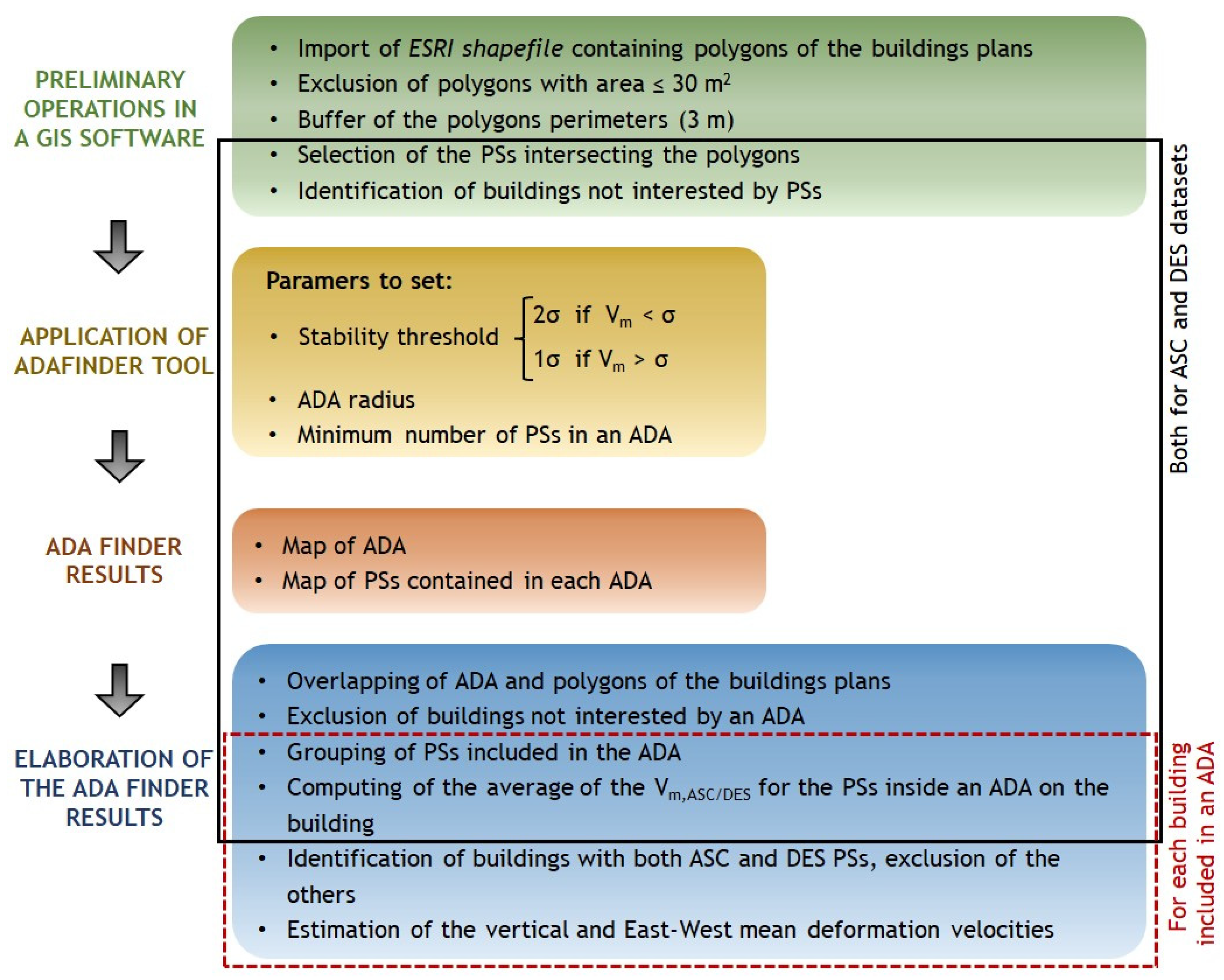
2.3. Proposed Methodology

The proposed methodology is focused on finding buildings interested by deformations above an established threshold, in urbanized areas characterized by large dataset of PSs, through ADAfinder tool. The latter is included in a procedure that, for the first time, is specific for urban districts or whole municipalities/towns. A flowchart of the proposed methodology is shown in Figure 1. The necessary data to implement the procedure are: (i) an ESRI shapefile containing the polygons of the buildings plans and (ii) the two datasets referred to ASC and DES orbits, containing information about the PSs of the monitored area.
Since the proposed methodology is dedicated to data processing for SHM purposes, the introduction in the flowchart of preliminary operations to be performed in a GIS software, listed in the green box of the flowchart, is needed. The preliminary operations are aimed to PSs datasets filtering to direct the procedure towards the analysis of ADAs on the buildings. First, the ESRI shapefile containing polygons of the buildings plans is imported. The polygons with an area lower than 30 m2 are excluded, since they are not considered to be buildings. In fact, sometimes, other little elements can be included in the available shapefiles, for example cabins, canopies, small buildings, silos, or containers in harbor areas. Then, a buffer of the polygons perimeters is done in order to take into account the inaccuracies that they might have. Since the presented methodology is focused on the buildings, all the PSs related to any other construction or reflective target have to be discarded. For this reason, a selection of the PSs intersecting the polygons (including the buffer previously mentioned) is done, while the buildings not intersected by PSs are identified and pointed out. In future, a minimum number of points, such as their distribution on the building plan, could also be added as preliminary filter of the procedure, to exclude from the analysis the buildings not well represented.
Then, all the operations included in the black contour in Figure 1 are separately done using both the ASC and DES datasets.
The following step is the application of the ADAfinder tool (yellow box of the flowchart). A criterion to establish the value of the stability threshold is to compare the Vm of the dataset of PSs with the relative σ. The original source of this criterion is to assume the stability threshold at 2σ to exclude all the points with lower Vm, as described in Barra et al. [35]. Herein, a more conservative additional constraint is assumed, since the final goal is the identification of the critical constructions. In fact, the stability threshold is set at (i) 2σ if Vm < σ, while it is set at (ii) 1σ if Vm > σ. In general, if a high average value of the velocity is present (ii), it can be important to consider more constructions in the monitoring phase and then a lower threshold value can be fixed. In fact, in the case (i), the values of Vm are greater, and a trend of deformations more or less defined is present, so it is convenient to keep a larger number of PSs. In contrast, the case (i) usually verifies in large areas with different deformation processes included, so a great dispersion of the Vm values can be detected and a cut at 2σ is more convenient to exclude the lower deformation values.
Moreover, the ADA radius (in meters) should be set, and the minimum number of PSs in an ADA has to be imposed. In the proposed methodology, it is recommended to set the minimum number of PSs equal to the minimum value accepted by the tool, that, in the current version (ADAtools 2.0.3), is 3. The operation described until this step must be carried out both for the ASC and the DES datasets.
Then, for both orbits, the results of the ADAfinder tool are obtained (orange box of the flowchart), consisting in two maps: one with the ADA (a polygonal ESRI shapefile), and one with the PSs contained in each ADA (a point ESRI shapefile), as explained in Section 2.2. These products are spatially superimposed to the polygons of buildings, obviously, as they are obtained from the PSs previously selected on the basis of them.
Finally, the ADAfinder results elaborated in order to obtain the definitive maps with information reclassified in function of the buildings, following the steps listed in the blue box of the flowchart. First of all, the ADA are overlapped to the buildings’ plans. The buildings not included in an ADA or a portion of an ADA are discarded. The remaining buildings, or portions of them, are classified as “unstable”. For them, two groups of “unstable” PSs are recognized: the group of ASC and the group of DES PSs. Then, for each building (with adequate numbers of PS), the average of the Vm and the σ of the ASC and DES PSs is computed only for the PSs inside the interested ADA. In this way, finally, only two values of Vm are associated to each building, representing the average of the mean deformation velocity along the line of sight (LoS) of the unstable PSs falling on the building itself: one along ASC (Vm,ASC) and one along DES (Vm,DES) orbits. At this step, an intersection of the results deriving from the ASC and DES datasets is performed to identify the buildings overlapped by at least one ADA from the ASC and one ADA from the DES dataset. The buildings not having both ASC and DES information are excluded from the following steps of the procedure, since the availability of both orbits is necessary for the estimation of the vertical and E-W mean deformation velocity components. Then, the vertical and E-W components of the mean deformation velocity for each building are estimated according to the formulas described in Talledo et al. [15]. The north–south component cannot be calculated, due to the very low sensitivity of the InSAR to this displacement component, because of the approximately north–south orbit inclination of SAR satellites. All the operations included in the dashed red contour in Figure 1 are done separately for each building included in an ADA.
The final maps give a preliminary identification of constructions potentially critical from a structural engineering point of view in terms of deformation, which needs a more accurate level of SHM.
The steps of the illustrated methodology can be implemented by combining simple operations to execute in QGIS and algorithms written in a code language (e.g., Matlab), as will be presented later.

3. Experimental Results

Two case study areas including distinct typologies of buildings (characterized by different materials, dimensions, and structural schemes) have been considered in order to show the potential of the proposed methodology applied to different kinds of urban settlements. The first one is part of the Eixample neighborhood, while the second one is part of the industrial area near the harbor, known as Zona Franca. It is worth highlighting that the PSs used in the following applications are derived by the EGMS, illustrated in Section 2.1.
Eixample is a district that occupies the central part of the city of Barcelona (Spain), in an area of 7.45 km². It was built in the second half of the 19th century based on the design of Ildefons Cerdà. The area is conceived as a regular pattern formed by quadrangular blocks of 113.30 m per side (that occupy an area of about 12,500 m² each), trunked on the vertices with a bevel of 15 m, and separated by a regular pattern of avenues. The blocks are constituted by adjoining buildings, mainly jointed, predominantly in masonry, with an average height of 30 m. For the following application, an area of 0.45 km2 was selected, where the blocks are also crossed by the Avinguda Diagonal.
Zona Franca is a very large logistics and industrial area located in the Sants-Montjuïc district of Barcelona, near the harbor and the airport. This area was used for the construction of several factories during the industrialization period of Catalonia, in the middle of 1900. It is completely different for the Eixample, since the constructions in this area are predominantly large sheds with plan roofs, located without a planned scheme. An area of 17 km2 of Zona Franca was selected for the following application.

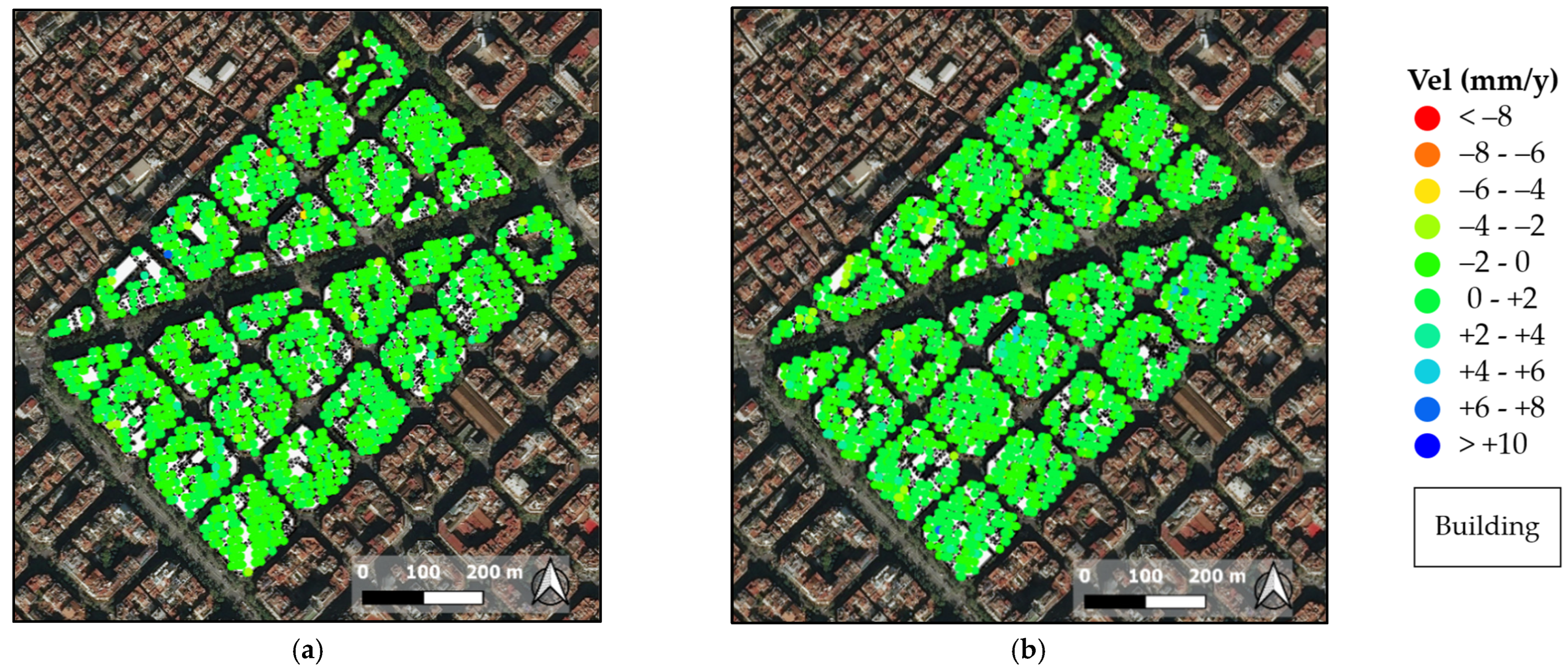
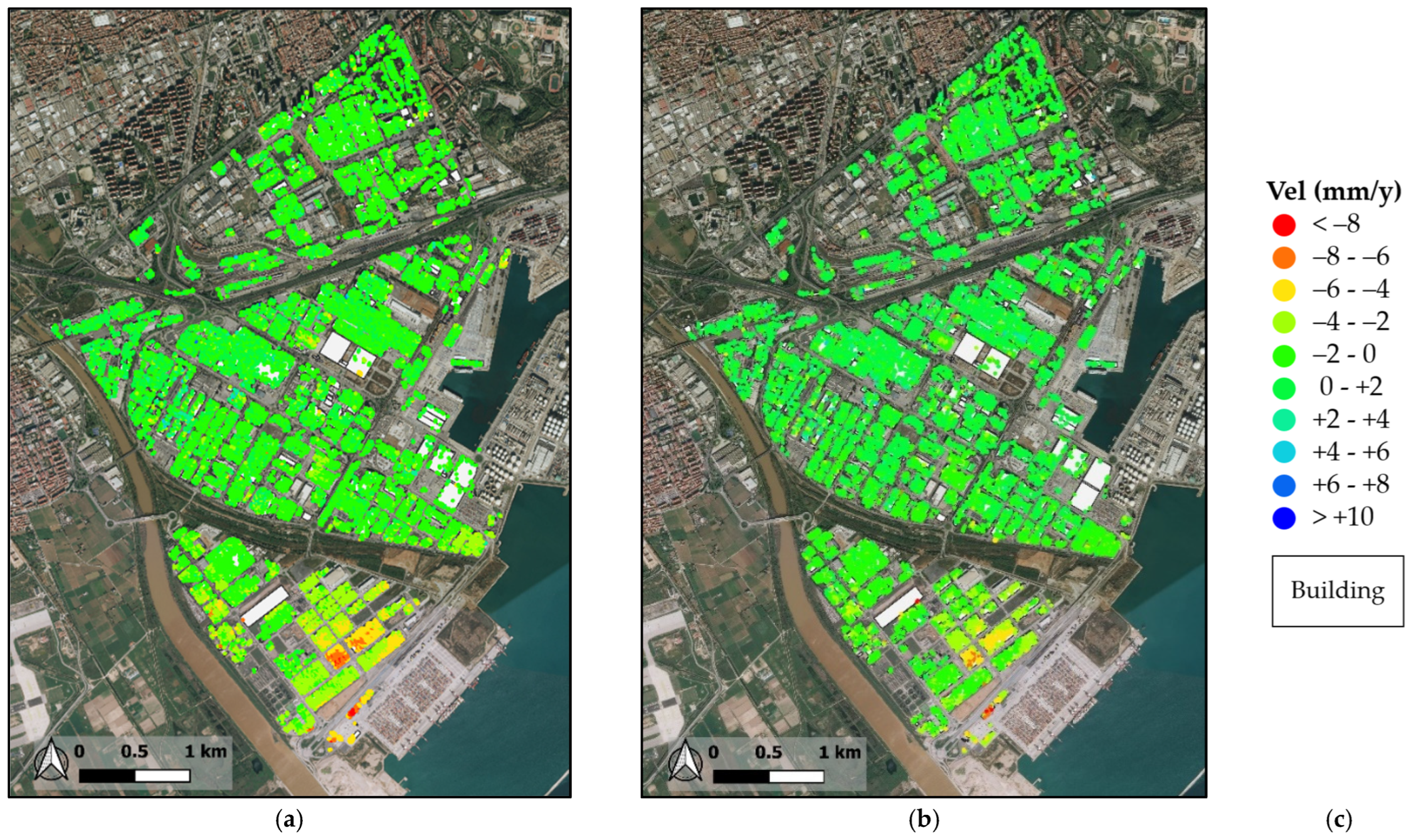
3.1. Preliminary Operations

The five steps of the first block of the flowchart in Figure 1 were performed for the two selected areas. The ESRI shapefile containing polygons of the building plans was downloaded from OpenStreetMap [44].
The distribution of the PSs in the area of the Eixample district is shown in Figure 2a,b, for ASC and DES orbits, respectively. In Table 1, the statistics of the mean velocity Vm of the PSs in the selected area are reported. It can be observed that the ASC PSs are more than the DES ones (almost 50% more), and that for both the datasets, the Vm is lower than the σ. The different number of PSs is probably due to the different viewing geometry of ASC and DES. The values of the Vm in this area are not significatively high, so the area can be considered stable. It is worth underlining, in fact, that this area was chosen for the configuration of the included constructions, and not for the entity of their deformation.
The distributions of the PSs in the area of the Zona Franca district are shown in Figure 3a,b, for ASC and DES orbits, respectively. Table 2 reports the statistics of the mean velocity Vm of the PSs in the selected area. Also in this case, it can be observed that the ASC PSs are many more of the DES ones (about 75% more), and that for both the datasets the Vm is lower than the σ. The values of the Vm in this area are greater, reaching, for example, −10.5 mm/y in moving away from the satellite along the ASC LoS. In particular, the greatest deformations can be observed in the southern part of the area, while the central and upper regions appear to be stable.
The urban structure of the two case study areas is very different. As mentioned before, the Eixample is characterized by the presence of adjoining buildings with small surface. In fact, about the 90% of the total number of buildings have an area lower than 1000 m2. In this case, over a total of 540 buildings, 524 are covered by at least 1 ASC PS and 532 are covered by at least one DES PS. However, all the buildings, except for two, are covered by a number of PSs greater than 4. In contrast, in the area of the Zona Franca district, almost half of the total number of buildings have an area greater than 1000 m2. Despite the larger size, there are many buildings that do not even have one PS. In fact, over a total of 1358 buildings, only 1198 are covered by at least one ASC PS and 1111 are covered by at least one DESC PS.
In Table 3, a summary of the number of monitorable buildings in the case study areas is reported. With respect to the total number of buildings, 4% of them are not covered by both ASC and DES PSs in Eixample. For Zona Franca, this percentage increased up to 23%. This effect could be related to the different viewing geometry of ASC and DES data and to the greater presence of reflecting elements in the area (e.g., antennas, parapets, balconies).

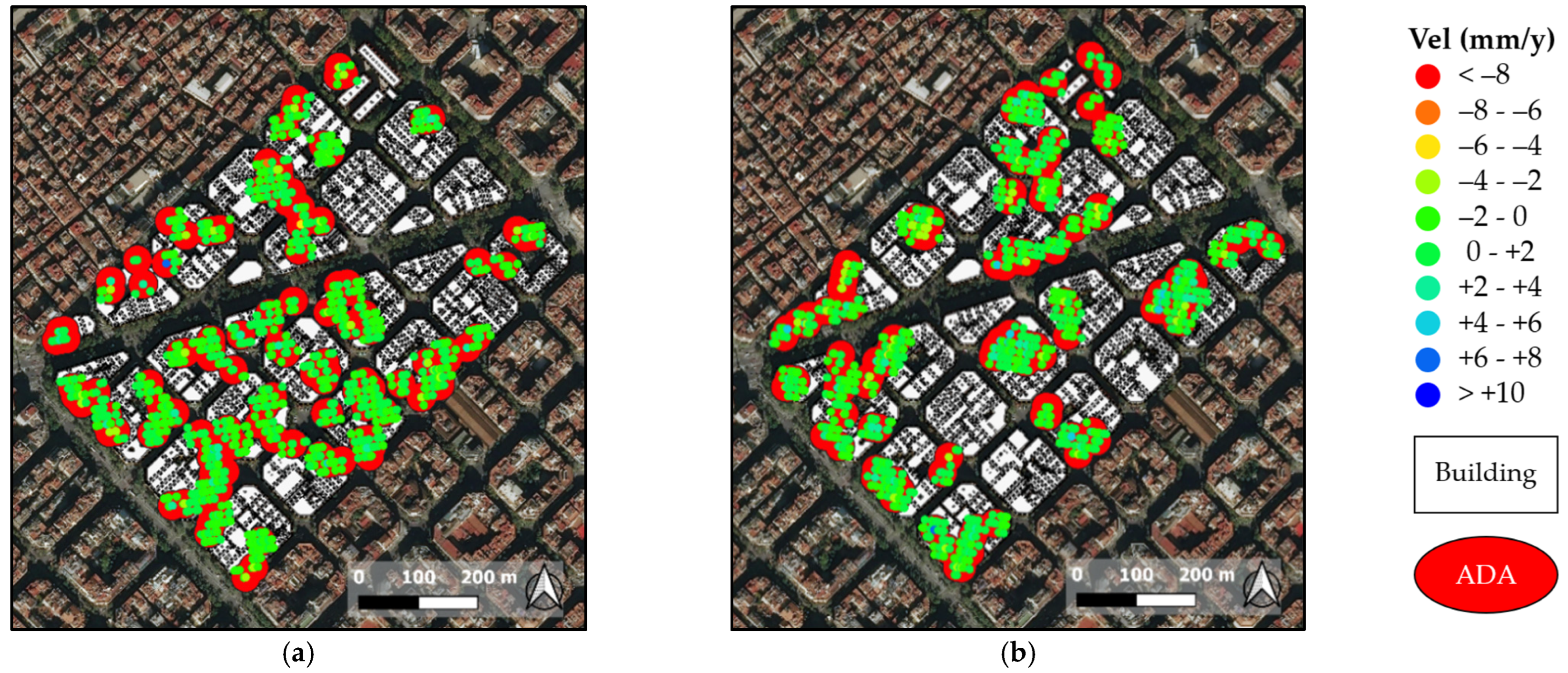
3.2. Application of ADAfinder Tool and Results

To obtain the ADA from the deformation maps shown in Figure 2 and Figure 3, the ADAfinder tool was applied, as explained in Section 2.3. Figure 4 and Figure 5 show the extracted ADA for both the orbits for the two case study areas. The polygons, colored in red for a better visualization, and the “active” PSs based on the velocity color scale, are represented. The definition of “active” depends on the stability threshold imposed on the Vm, that is area-dependent. In general, the stability threshold was set at 2σ, in accordance with what was explained in Section 2.3. Moreover, the ADA radius was set at 25 m and the minimum number of PSs to be included in an ADA was fixed to 3. It can be observed that the number of PSs over the areas was greatly reduced with respect to the input datasets (of Figure 2 and Figure 3). For the area of Eixample, only 75% of ASC and the 37% of DES PSs was preserved, while for the Zona Franca, the cut was even more drastic, with a loss of more than the 80% of PSs in both datasets. This largest cut was justified by the presence of different gradients of deformation in the considered portion of the Zona Franca, previously commented, with a greater variability of Vm values. In Table 4 and Table 5, the statistics of the Vm of the active PSs are also reported.
In Table 6, a summary of the number of buildings included in ADA for both ASC and DES datasets is reported. In Eixample area, a percentage greater than 50% was included in ADA, while in Zona Franca, this percentage was about 10%. The difference is due to the different velocity threshold, which is very low in the first area (because of its stability) and higher in the second area, where a significant sorting is done on buildings that are really deforming.

3.3. Elaboration of the ADAfinder Results

The attribute tables of the PSs included in each ASC or DES ADA are extended by associating the ID number of the building intersecting the PSs themselves. The average Vm,ASC and Vm,DES for each building are estimated. In the maps of Figure 6 and Figure 7, the average Vm,ASC and Vm,DES are shown coloring the buildings surfaces, respectively, for Eixample and for Zona Franca. The buildings characterized by lack of PSs are covered by violet polygons. The number of PSs used to compute the average Vm,ASC and Vm,DES for each building is important because the more points there are, the more reliable the measurement can be. For Eixample, this number varies between 2 and 82 for ASC and between 1 and 37 for DES. For Zona Franca, this number varies between 1 and 476 for ASC and between 1 and 169 for DES. The upper bound is a function of the dimension of the building surface.
The maps of vertical and E-W components of the mean deformation velocity (VV and VEW) are respectively shown in Figure 8a,b and in Figure 9a,b for the two case study areas. In these final maps, the union of the buildings characterized by lack of PSs in the original datasets is marked with violet polygons. It is important to remark this information because these buildings could be “unstable”, but they cannot be investigated using the presented methodology. Further study should be done to estimate their deformation condition.
The final number of monitored buildings is 140 for Eixample and 75 for Zona Franca. The velocity component maps remark that the area of Eixample is stable. In contrast, in the southern part of the Zona Franca, there are buildings affected by vertical deformations. In particular, 3 buildings reach vertical downwards average velocities included between 8 and 10 mm/y, another 3 between 6 and 8 mm/y, but the most populated velocity range is between 4 and 6 mm/y, with 20 buildings affected by vertical velocities of this entity.
A focus on one of the quadrangular blocks of the Eixample is reported in Figure 10a,b for ASC and DES PSs, respectively. Figure 10c shows the consequent map of vertical/E-W components of the mean deformation velocity (in this case, because of the stability of the buildings, the two maps are equal, characterized by green color).

4. Discussion

In this section, potential and limitations of the proposed methodology for deformations/structural monitoring of urban settlements are discussed.
First of all, regarding the ESRI shapefile containing the buildings plans, it is worth noting that OpenStreetMap constitutes a convenient service, free and open, for users worldwide. Nevertheless, the provided shapefiles are manually created by a community of contributing mappers, so may contain approximations or imprecisions. By improving the accuracy of the input ESRI shapefile containing the buildings plans, the accuracy of the results could also increase. If geometrical reliefs of the area are available, they can be included in the procedure.
The ADAfinder tool has been applied to datasets of PSs subjected to pre-processing operations. This kind of application somewhat departs from the original use of the tool because the aim is different, since it is focuses only on the buildings. In fact, in the cited applications (e.g., Barra et al. [35]), the input PSs dataset is usually referred to an entire area, without any pre-selection. Then, the identified ADA refers to any part of the area under monitoring. In this work, instead, the structure of the desired results is opportunely channeled, in order to obtain information related to the buildings, and, in particular, to each building affected by deformations exceeding the imposed velocity threshold.
The final maps of the vertical and E-W velocity components contain one value for each “active building”. On one hand, this could appear simplistic, giving limited information. On the other hand, considering the great dimensions of the areas where the proposed methodology could be applied, that could be districts, municipalities, towns, these final synthetic maps give precious preliminary information about the most critical buildings of the area.
From a structural engineering point of view, it is important to investigate the two components of deformations, since they can induce different structural response in the buildings, with different levels of hazard. This theme has been deeply studied by Miano et al. [45].
Moreover, it is worth highlighting that the resolution of the Sentinel-1 data is not sufficient to perform detailed analysis at the scale of single buildings. Then, the component velocity maps could be used as a preliminary tool to identify buildings that are affected by significant deformations and need to be further investigated.
Some of the possible investigation strategies to carry out are only briefly cited in this work, since they fall outside of its scope. For example, surveys to ascertain the conditions of these buildings could be done, and, if necessary, on-site monitoring could be provided. If other kind of satellite data, with higher resolution with respect to the Sentinel-1, are available, it is also possible to integrate the procedure by analyzing the critical buildings at single scale adopting other approaches [11,15].
The procedure can be repeated yearly, every time that the EGMS data are updated. This can guarantee not only a monitoring of the absolute value of the velocity/displacements on the whole time, but also differential comparisons between the velocity for each year, establishing additional thresholds of alert on the maximum acceptable values of variation.
The two case study areas have different urbanistic features, concerning the dimensions and distribution of the included buildings. This reflects in the PSs covering, as deeply explained in Section 3.1. The applications show that not all the buildings of the chosen areas are monitorable. In fact, when no PS intersects the building plan, as well as if the building is intersected only by PSs along one single orbit, that building is automatically excluded. The absence of PS should not be interpreted as absence of movement. It could be related to the decorrelation effects [46] that could provide a lack of deformation measurement points. Another reason could be the presence of anomalies in the deformation signal, such as to lead to very low values of the temporal coherence due to the estimation of PSs displacement time series characterized by a strong variability in time. However, if the unmonitored building is rounded by a significant number of other buildings with significant deformations, one idea could be to use an Inverted Distance Weighted (IDW) approach [47], by achieving the velocity vertical and horizontal components for the building from the linear interpolation of the other buildings.
An important parameter to consider is the number of PSs on each building. Theoretically, the methodology works when the number of ASC and DES PSs is almost 1 for each building, but the reliability of the results increases when the number of PSs increases.
The results for the area of Eixample, shown in Figure 8, highlight that a difficulty can be found in reading the final maps, because of the fact that the buildings are very close one to each other and have very small plans (even if they develop in height). This reading difficulty could be seen as a limitation, but it is not relevant, if thinking about the fact that it is expected that buildings so close will have the same deformation trends, at least if the cause concerns a deformation phenomenon of the underlying soil, which therefore affects the foundations.

5. Conclusions

In this paper, a methodology based on the use of the ADAfinder tool for the monitoring of the deformative condition of the constructions in urban areas was proposed. The methodology can be performed using satellite SAR data derived by every satellite constellation, processed with any existing processing techniques. In this work, EGMS data were used to demonstrate their great potential in applications regarding the structural monitoring at large scale. It is worth remembering that Sentinel-1 satellite data are cost-free, so their use could be preferable to other satellite data thinking about long-term monitoring at large scale. Nevertheless, the number of PSs over small buildings could increase by using SAR satellite data obtained by processing SAR images with higher resolution, as those derived by the COSMO-SkyMed constellation. The main output are the velocity maps along the vertical and E-W directions, which condense the most significant information about the deformation of the buildings included in the deformation-active areas. These products are very clear, simple, and useful, and could provide real support for the management of the urban areas.
The potentialities of the proposed methodology have been shown out of its application over two zones of Barcelona (Spain), very distinct for the configuration and for the features of the buildings. The chosen zones include rather small groups of buildings for three reasons. First of all, for the preliminary identification of constructions potentially critical from a structural engineering point of view (e.g., affected by high values of settlements), that need a more accurate level of SHM (e.g., exploiting the PSs points belonging to the selected construction to check also the presence of differential displacements, and then integrating the knowledge with in situ monitoring techniques). The second reason is that the presented applications have been useful to test the proposed methodology at all its steps, facing different problems related to the different characteristics of the two areas. Finally, to work with small areas implies that, for instance, if there is just one building exposed to a local issue in a stable zone, the ADA tool certainly identifies this building as critical. The same building, in a greater zone with uniform high levels of displacements, could be discarded based on the velocity threshold estimated based on the total measures of the wide area. However, as the ADA tool is focused on finding active deformation on a wide area and a large dataset, coarse scale analysis that includes an entire city, e.g., all the Barcelona municipalities, could enhance the potentiality of the tool (by also checking the previous described situation). This is a larger goal that will be pursued in the next future.
The procedure could be improved introducing a classification of the buildings, based on structural features (e.g., the building material, the number of floors, or the construction period), and giving a velocity threshold specific for each class.
It is important to keep on working on providing tools, methodologies, or indications in general, about how to manage and use the EGMS data, which constitute a great opportunity for the large user population that could benefit from them.

Author Contributions

Conceptualization, A.M. (Annalisa Mele), M.C., A.M. (Andrea Miano) and A.P.; formal analysis, A.M. (Annalisa Mele), M.C. and A.M. (Andrea Miano); methodology, A.M. (Annalisa Mele), M.C. and A.M. (Andrea Miano); supervision, M.C. and A.P.; validation, A.M. (Annalisa Mele), M.C. and A.M. (Andrea Miano); writing—original draft, A.M. (Annalisa Mele) and A.M. (Andrea Miano); writing—review and editing, A.M. (Annalisa Mele), M.C. and A.M. (Andrea Miano). All authors have read and agreed to the published version of the manuscript.

Funding

This research received no external funding.

Data Availability Statement

The SAR satellite data used in this work are from the European Gound Motion Service. They are public and available.

Acknowledgments

The first author visited the Centre Tecnològic de Telecomunicacions de Catalunya (CTTC/CERCA) to conduct part of the presented research. Her visit was funded by the University of Naples Federico II in the framework of the Ph.D. program in Structural Engineering, Geotechnics and Seismic Risk. This support is gratefully acknowledged. This work is part of the Spanish Grant SARAI, PID2020-116540RB-C21.

Conflicts of Interest

The authors declare no conflict of interest.

References

  1. Tomás, R.; Li, Z. Earth Observations for Geohazards: Present and Future Challenges. Remote Sens. 2017, 9, 194. [Google Scholar] [CrossRef] [Green Version]
  2. Bianchini, S.; Raspini, F.; Solari, L.; Del Soldato, M.; Ciampalini, A.; Rosi, A.; Casagli, N. From Picture to Movie: Twenty Years of Ground Deformation Recording Over Tuscany Region (Italy) with Satellite InSAR. Front. Earth Sci. 2018, 6, 177. [Google Scholar] [CrossRef] [Green Version]
  3. Raucoules, D.; Colesanti, C.; Carnec, C. Use of SAR interferometry for detecting and assessing ground subsidence. C. R. Geosci. 2007, 339, 289–302. [Google Scholar] [CrossRef]
  4. Costantini, M.; Ferretti, A.; Minati, F.; Falco, S.; Trillo, F.; Colombo, D.; Novali, F.; Malvarosa, F.; Mammone, C.; Vecchioli, F.; et al. Analysis of surface deformations over the whole Italian territory by interferometric processing of ERS, Envisat and COSMO-SkyMed radar data. Remote Sens. Environ. 2017, 202, 250–275. [Google Scholar] [CrossRef]
  5. Tomás, R.; Romero, R.; Mulas, J.; Marturià, J.J.; Mallorquí, J.J.; Lopez-Sanchez, J.M.; Herrera, G.; Gutiérrez, F.; González, P.J.; Fernández, J.; et al. Radar interferometry techniques for the study of ground subsidence phenomena: A review of practical issues through cases in Spain. Environ. Earth Sci. 2017, 71, 163–181. [Google Scholar] [CrossRef] [Green Version]
  6. Reale, D.; Fornaro, G.; Pauciullo, A.; Zhu, X.; Bamler, R. Tomographic imaging and monitoring of buildings with very high resolution SAR data. IEEE Geosci. Remote Sens. Lett. 2011, 8, 661–665. [Google Scholar] [CrossRef] [Green Version]
  7. Arangio, S.; Calò, F.; Di Mauro, M.; Bonano, M.; Marsella, M.; Manunta, M. An application of the SBAS-DInSAR technique for the assessment of structural damage in the city of Rome. Struct. Infrastruct. Eng. 2013, 10, 1469–1483. [Google Scholar] [CrossRef]
  8. Bianchini, S.; Pratesi, F.; Nolesini, T.; Casagli, N. Building deformation assessment by means of persistent scatterer interferometry analysis on a landslide affected area: The Volterra (Italy) case study. Remote Sens. 2015, 7, 4678–4701. [Google Scholar] [CrossRef] [Green Version]
  9. Chen, F.; Zhou, W.; Chen, C.; Ma, P. Extended D-TomoSAR Displacement Monitoring for Nanjing (China) City Built Structure Using High-Resolution TerraSAR/TanDEM-X and Cosmo SkyMed SAR Data. Remote Sens. 2019, 11, 2623. [Google Scholar] [CrossRef] [Green Version]
  10. Cusson, D.; Rossi, C.; Ozkan, I.F. Early warning system for the detection of unexpected bridge displacements from radar satellite data. J. Civ. Struct. Health Monit. 2021, 11, 189–204. [Google Scholar] [CrossRef]
  11. Di Carlo, F.; Miano, A.; Giannetti, I.; Mele, A.; Bonano, M.; Lanari, R.; Meda, A.; Prota, A. On the integration of multi-temporal synthetic aperture radar interferometry products and historical surveys data for buildings structural monitoring. J. Civ. Struct. Health Monit. 2021, 11, 1–19. [Google Scholar] [CrossRef]
  12. Miano, A.; Mele, A.; Calcaterra, D.; Di Martire, D.; Infante, D.; Prota, A.; Ramondini, M. The use of satellite data to support the structural health monitoring in areas affected by slow-moving landslides: A potential application to reinforced concrete buildings. Struct. Health Monit. 2021, 20, 3265–3287. [Google Scholar] [CrossRef]
  13. Mele, A.; Miano, A.; Di Martire, D.; Infante, D.; Ramondini, M.; Prota, A. Potential of remote sensing data to support the seismic safety assessment of reinforced concrete buildings affected by slow-moving landslides. Arch. Civ. Mech. Eng. 2022, 22, 88. [Google Scholar] [CrossRef]
  14. Miano, A.; Di Carlo, F.; Mele, A.; Giannetti, I.; Nappo, N.; Rompato, M.; Striano, P.; Bonano, M.; Bozzano, F.; Lanari, R.; et al. GIS Integration of DInSAR Measurements, Geological Investigation and Historical Surveys for the Structural Monitoring of Buildings and Infrastructures: An Application to the Valco San Paolo Urban Area of Rome. Infrastructures 2022, 7, 89. [Google Scholar] [CrossRef]
  15. Talledo, D.A.; Miano, A.; Bonano, M.; Di Carlo, F.; Lanari, R.; Manunta, M.; Meda, A.; Mele, A.; Saeta, A.; Stella, A. Satellite radar interferometry: Potential and limitations for structural assessment and monitoring. J. Build. Eng. 2022, 46, 103756. [Google Scholar] [CrossRef]
  16. Ferretti, A.; Prati, C.; Rocca, F.; Wasowski, J. Satellite interferometry for monitoring ground deformations in the urban environment. In Proceedings of the 10th IAEG Congress, Nottingham, UK, 6–10 September 2006; pp. 100–110. [Google Scholar]
  17. Manunta, M.; Marsella, M.; Zeni, G.; Sciotti, M.; Atzori, S.; Lanari, R. Two-scale surface deformation analysis using the SBAS-DInSAR technique: A case study of the city of Rome, Italy. Int. J. Remote Sens. 2008, 29, 1665–1684. [Google Scholar] [CrossRef]
  18. Stramondo, S.; Bozzano, F.; Marra, F.; Wegmuller, U.; Cinti, F.R.; Moro, M.; Saroli, M. Subsidence induced by urbanisation in the city of Rome detected by advanced InSAR technique and geotechnical investigations. Remote Sens. Environ. 2008, 112, 3160–3172. [Google Scholar] [CrossRef]
  19. Infante, D.; Confuorto, P.; Di Martire, D.; Ramondini, M.; Calcaterra, D. Use of DInSAR data for multi-level vulnerability assessment of urban settings affected by slow-moving and intermittent landslides. Procedia Eng. 2016, 158, 470–475. [Google Scholar] [CrossRef] [Green Version]
  20. Peduto, D.; Nicodemo, G.; Maccabiani, J.; Ferlisi, S. Multi-scale analysis of settlement-induced building damage using damage surveys and DInSAR data: A case study in the Netherlands. Eng. Geol. 2017, 218, 117–133. [Google Scholar] [CrossRef]
  21. Macchiarulo, V.; Milillo, P.; DeJong, M.J.; González Martí, J.; Sánchez, J.; Giardina, G. Integrated InSAR monitoring and structural assessment of tunnelling-induced building deformations. Struct. Control Health 2021, 28, 9. [Google Scholar] [CrossRef]
  22. Dehls, J.F.; Larsen, Y.; Marinkovic, P.; Lauknes, T.R.; Stødle, D.; Moldestad, D.A. INSAR. No: A National Insar Deformation Mapping/Monitoring Service in Norway-From Concept to Operations. In Proceedings of the IGARSS 2019—2019 IEEE International Geoscience and Remote Sensing Symposium, Yokohama, Japan, 28 July–2 August 2019; pp. 5461–5464. [Google Scholar] [CrossRef]
  23. Kalia, A.C.; Frei, M.; Lege, T. A Copernicus downstream-service for the nationwide monitoring of surface displacements in Germany. Remote Sens. Environ. 2017, 202, 234–249. [Google Scholar] [CrossRef]
  24. Raspini, F.; Bianchini, S.; Ciampalini, A.; Del Soldato, M.; Solari, L.; Novali, F.; Del Conte, S.; Rucci, A.; Ferretti, A.; Casagli, N. Continuous, semi-automatic monitoring of ground deformation using Sentinel-1 satellites. Sci. Rep. 2018, 8, 7253. [Google Scholar] [CrossRef] [PubMed] [Green Version]
  25. Del Soldato, M.; Solari, L.; Raspini, F.; Bianchini, S.; Ciampalini, A.; Montalti, R.; Ferretti, A.; Pellegrineschi, V.; Casagli, N. Monitoring Ground Instabilities Using SAR Satellite Data: A Practical Approach. ISPRS Int. J. Geo-Inf. 2019, 8, 307. [Google Scholar] [CrossRef] [Green Version]
  26. Solari, L.; Del Soldato, M.; Montalti, R.; Bianchini, S.; Raspini, F.; Thuegaz, P.; Bertolo, D.; Tofani, V.; Casagli, N. A Sentinel-1 based hot-spot analysis: Landslide mapping in north-western Italy. Int. J. Remote Sens. 2019, 40, 7898–7921. [Google Scholar] [CrossRef]
  27. Crosetto, M.; Solari, L.; Mróz, M.; Balasis-Levinsen, J.; Casagli, N.; Frei, M.; Oyen, A.; Moldestad, D.A.; Bateson, L.; Guerrieri, L.; et al. The evolution of wide-area DInSAR: From regional and national services to the European Ground Motion Service. Remote Sens. 2020, 12, 2043. [Google Scholar] [CrossRef]
  28. Crosetto, M.; Solari, L.; Balasis-Levinsen, J.; Casagli, N.; Frei, M.; Oyen, A.; Moldestad, D.A. Ground deformation monitoring at continental scale: The European Ground Motion Service. Int. Arch. Photogramm. Remote Sens. Spat. Inf. Sci. 2020, 43, 293–298. [Google Scholar] [CrossRef]
  29. Costantini, M.; Minati, F.; Trillo, F.; Ferretti, A.; Novali, F.; Passera, E.; Dehls, J.; Larsen, Y.; Marinkovic, P.; Eineder, M.; et al. European Ground Motion Service (EGMS). In Proceedings of the 2021 IEEE International Geoscience and Remote Sensing Symposium IGARSS, Brussels, Belgium, 11–16 July 2021; pp. 3293–3296. [Google Scholar]
  30. Crosetto, M.; Solari, L.; Balasis-Levinsen, J.; Bateson, L.; Casagli, N.; Frei, M.; Oyen, A.; Moldestad, D.A.; Mróz, M. Deformation Monitoring at European Scale: The Copernicus Ground Motion Service. Int. Arch. Photogramm. Remote Sens. Spat. Inf. Sci. 2021, 43, 141–146. [Google Scholar] [CrossRef]
  31. Meisina, C.; Zucca, F.; Notti, D.; Colombo, A.; Cucchi, A.; Savio, G.; Giannico, C.; Bianchi, M. Geological Interpretation of PSInSAR Data at Regional Scale. Sensors 2008, 8, 7469–7492. [Google Scholar] [CrossRef] [Green Version]
  32. Bianchini, S.; Cigna, F.; Righini, G.; Proietti, C.; Casagli, N. Landslide HotSpot Mapping by means of Persistent Scatterer Interferometry. Environ. Earth Sci. 2012, 67, 1155–1172. [Google Scholar] [CrossRef]
  33. Solari, L.; Barra, A.; Herrera, G.; Bianchini, S.; Monserrat, O.; Béjar-Pizarro, M.; Crosetto, M.; Sarro, R.; Moretti, S. Fast detection of ground motions on vulnerable elements using Sentinel-1 InSAR data. Geomat. Nat. Hazards Risk. 2018, 9, 152–174. [Google Scholar] [CrossRef] [Green Version]
  34. Mele, A.; Vitiello, A.; Bonano, M.; Miano, A.; Lanari, R.; Acampora, G.; Prota, A. On the Joint Exploitation of Satellite DInSAR Measurements and DBSCAN-Based Techniques for Preliminary Identification and Ranking of Critical Constructions in a Built Environment. Remote Sens. 2022, 14, 1872. [Google Scholar] [CrossRef]
  35. Barra, A.; Solari, L.; Béjar-Pizarro, M.; Monserrat, O.; Bianchini, S.; Herrera, G.; Crosseto, M.; Sarro, R.; Gonzales-Alonso, E.; Mateos, R.M.; et al. A methodology to detect and update active deformation areas based on sentinel-1 SAR images. Remote Sens. 2017, 9, 1002. [Google Scholar] [CrossRef] [Green Version]
  36. Navarro, J.A.; Tomás, R.; Barra, A.; Pagán, J.I.; Reyes-Carmona, C.; Solari, L.; Vinielles, J.L.; Falco, S.; Crosetto, M. ADAtools: Automatic detection and classification of active deformation areas from PSI displacement maps. ISPRS Int. J. Geo-Inf. 2020, 9, 584. [Google Scholar] [CrossRef]
  37. EGMS White Paper. Available online: https://land.copernicus.eu/user-corner/technical-library/egms-white-paper (accessed on 14 June 2022).
  38. CLSM. Available online: https://www.copernicus.eu/en/copernicus-services/land (accessed on 14 June 2022).
  39. Crosetto, M.; Monserrat, O.; Cuevas-González, M.; Devanthéry, N.; Crippa, B. Persistent Scatterer Interferometry: A review. ISPRS J. Photogramm. Remote Sens. 2016, 115, 78–89. [Google Scholar] [CrossRef] [Green Version]
  40. Ferretti, A.; Passera, E.; Capes, R. Algorithm Theoretical Basis Document. EGMS Documentation. 2021. Available online: https://land.copernicus.eu/user-corner/technical-library/egms-algorithm-theoretical-basis-document (accessed on 1 March 2022).
  41. Kotzerke, P.; Siegmund, R.; Langenwalter, J. Product User Manual. EGMS Documentation. 2022. Available online: https://land.copernicus.eu/user-corner/technical-library/egms-product-user-manual (accessed on 1 March 2022).
  42. Tomás, R.; Pagán, J.I.; Navarro, J.A.; Cano, M.; Pastor, J.L.; Riquelme, A.; Cuevas-Gonzales, M.; Crosseto, M.; Barra, A.; Monserrat, O.; et al. Semi-automatic identification and pre-screening of geological–geotechnical deformational processes using persistent scatterer interferometry datasets. Remote Sens. 2019, 11, 1675. [Google Scholar] [CrossRef] [Green Version]
  43. Ferretti, A.; Monti-Guarnieri, A.; Prati, C.; Rocca, F.; Massonet, D. InSAR Principles-Guidelines for SAR Interferometry Processing and Interpretation, TM-19; ESA Publications: Auckland, New Zealand, 2007. [Google Scholar]
  44. OpenStreetMap. Available online: https://www.openstreetmap.org/ (accessed on 25 March 2022).
  45. Miano, A.; Mele, A.; Prota, A. Fragility curves for different classes of existing RC buildings under ground differential settlements. Eng. Struct. 2022, 257, 114077. [Google Scholar] [CrossRef]
  46. Zebker, H.A.; Villasenor, J. Decorrelation in interferometric radar echoes. IEEE Trans. Geosci. Remote Sens. 1992, 30, 950–959. [Google Scholar] [CrossRef] [Green Version]
  47. Lu, G.Y.; Wong, D.W. An adaptive inverse-distance weighting spatial interpolation technique. Comput. Geosci. 2008, 34, 1044–1055. [Google Scholar] [CrossRef]
Figure 1. Flowchart of the proposed methodology.
Remotesensing 15 00324 g001
Figure 2. Distribution of the selected PSs on the buildings of the selected area of Eixample: (a) ascending and (b) descending.
Remotesensing 15 00324 g002
Figure 3. Distribution of the selected PSs on the buildings of the selected area of Zona Franca: (a) ascending and (b) descending. (c) statistics of the mean velocity Vm of the selected area.
Remotesensing 15 00324 g003
Figure 4. ADA extraction from the active PSs of the selected area of Eixample from (a) ascending and (b) descending datasets.
Remotesensing 15 00324 g004
Figure 5. ADA extraction from the active PSs of the selected area of Zona Franca from (a) ascending and (b) descending datasets.
Remotesensing 15 00324 g005
Figure 6. Maps of buildings in Eixample area with an average value of mean deformation velocity along (a) ascending and (b) descending orbit. The violet polygons represent buildings with lack of PSs.
Remotesensing 15 00324 g006
Figure 7. Maps of buildings in Zona Franca area with an average value of mean deformation velocity along (a) ascending and (b) descending orbit. The violet polygons represent buildings with lack of PSs.
Remotesensing 15 00324 g007
Figure 8. Maps of (a) VEW and (b) VV components for the “unstable” buildings in Eixample area. The violet polygons represent buildings with original lack of PSs.
Remotesensing 15 00324 g008
Figure 9. Maps of (a) VEW and (b) VV components for the “unstable” buildings in Zona Franca area. The violet polygons represent buildings with original lack of PSs.
Remotesensing 15 00324 g009
Figure 10. Maps of average values of mean deformation velocity along (a) ascending and (b) descending orbit, and (c) map of VEW/v components for one of the quadrangular blocks of the Eixample. The labels indicate the number of PSs used to compute the average mean deformation velocities for each specific building.
Remotesensing 15 00324 g010
Table 1. Statistics of the mean velocity Vm (mm/y) of the selected area of Eixample.
CountMinimum VmMaximum VmAverage Vmσ
Ascending6389−7.306.600.110.82
Descending4347−6.207.300.150.94
Table 2. Statistics of the mean velocity Vm (mm/y) of the selected area of Zona Franca.
CountMinimum VmMaximum VmAverage Vmσ
Ascending33,965−10.506.90−0.901.54
Descending19,333−8.607.70−0.121.35
Table 3. Summary of the number of buildings in the case study areas.
EixampleZona Franca
Total number of buildings5401358
% of buildings with no ASC PSs3%12%
% of buildings with no DESC PSs1%18%
% of monitorable buildings96%77%
Table 4. Statistics of the mean velocity Vm (mm/y) of the active PSs of the selected area of Eixample.
CountMinimum VmMaximum VmAverage Vmσ
Ascending4800−7.306.900.121.06
Descending1624−6.207.300.151.28
Table 5. Statistics of the mean velocity Vm (mm/y) of the active PSs of the selected area of Zona Franca.
CountMinimum VmMaximum VmAverage Vmσ
Ascending6333−10.506.80−2.822.15
Descending2248−8.607.70−1.502.49
Table 6. Summary of the number of buildings in the case study areas.
EixampleZona Franca
Total number of buildings5401358
% of buildings included in an ASC ADA54%13%
% of buildings included in a DES ADA53%10%
Disclaimer/Publisher’s Note: The statements, opinions and data contained in all publications are solely those of the individual author(s) and contributor(s) and not of MDPI and/or the editor(s). MDPI and/or the editor(s) disclaim responsibility for any injury to people or property resulting from any ideas, methods, instructions or products referred to in the content.

