Abstract
In the last few years, there has been a renewed interest in data fusion techniques, and, in particular, in pansharpening due to a paradigm shift from model-based to data-driven approaches, supported by the recent advances in deep learning. Although a plethora of convolutional neural networks (CNN) for pansharpening have been devised, some fundamental issues still wait for answers. Among these, cross-scale and cross-datasets generalization capabilities are probably the most urgent ones since most of the current networks are trained at a different scale (reduced-resolution), and, in general, they are well-fitted on some datasets but fail on others. A recent attempt to address both these issues leverages on a target-adaptive inference scheme operating with a suitable full-resolution loss. On the downside, such an approach pays an additional computational overhead due to the adaptation phase. In this work, we propose a variant of this method with an effective target-adaptation scheme that allows for the reduction in inference time by a factor of ten, on average, without accuracy loss. A wide set of experiments carried out on three different datasets, GeoEye-1, WorldView-2 and WorldView-3, prove the computational gain obtained while keeping top accuracy scores compared to state-of-the-art methods, both model-based and deep-learning ones. The generality of the proposed solution has also been validated, applying the new adaptation framework to different CNN models.
1. Introduction
Due to the increasing number of remote sensing satellites and to renewed data sharing policies, e.g., the European Space Agency (ESA) Copernicus program, the remote sensing community calls for new data fusion techniques for such diverse applications as cross-sensor [1,2,3,4], cross-resolution [5,6,7,8] or cross-temporal [4,9,10] ones, for analysis, information extraction or synthesis tasks. In this work, we target the pansharpening of remotely sensed images, which amounts to the fusion of a single high resolution panchromatic (PAN) band with a set of low resolution multispectral (MS) bands to provide a high-resolution MS image.
A recent survey [11] gathered the available solutions in four categories: component substitution (CS) [12,13,14,15], multiresolution analysis (MRA) [16,17,18,19], variational optimization (VO) [20,21,22,23], and machine/deep learning (ML) [24,25,26,27,28]. In the CS approach, the multispectral image is transformed in a suitable domain, one of its components is replaced by the spatially rich PAN and the image is transformed back into the original domain. For example, in the simple case where only three spectral bands are concerned, the Intensity-Hue-Saturation (IHS) transform can be used for this purpose. The same method has been straightforwardly generalized to the case of a larger number of bands in [13]. Other examples of this approach, to mention a few, are whitening [12], Brovey [14] or the Gram–Schmidt decomposition [15]. In the MRA approach, instead, pansharpening is addressed resorting to a multi-resolution decomposition, such as decimated or undecimated wavelet transforms [16,18] and Laplacian pyramids [17,19], for proper extraction of the detail component to be injected into the resized multispectral component. VO approaches leverage on suitable acquisition or representation models to define a target function to optimize. This can involve the degradation filters mapping high-resolution to low-resolution images [22], sparse representation of the injected details [29], probabilistic models [21] and low-rank PAN-MS representations [23]. Needless to say, the paradigm shift from model-based to ML approaches registered in the last decade has also heavily had an impact on such diverse remote sensing-related image processing problems as classification, detection, denoising, data fusion and so forth. In particular, the first pansharpening convolutional neural network (PNN) was introduced by Masi et al. (2016) [24], and it was rapidly followed by many other works [25,27,28,30,31,32].
It seems safe to say that deep learning is currently the most popular approach for pansharpening. Nonetheless, it suffers from a major problem: the lack of ground truth data for supervised training. Indeed, multiresolution sensors can only provide the original MS-PAN data, downgraded in space or spectrum, never their high-resolution versions, which remain to be estimated. The solution to this problem introduced in [24], and still adopted by many others, consists in a resolution shift. The resolution of the PAN-MS data is properly downgraded by a factor equal to the PAN-MS resolution ratio in order to obtain input data whose ground-truth (GT) is given by the original MS. Any network can therefore be trained in a fully supervised manner, although in a lower-resolution domain, and then be used on full-resolution images at inference time. The resolution downgrade paradigm is not new, as it stems from Wald’s protocol [33], a procedure employed in the contest of the pansharpening quality assessment, and presents two main drawbacks:
- i.
- It requires the knowledge of the point spread function (also referred to as sensor Modulation Transfer Function, MTF, in the pansharpening context), which characterizes the imaging system, to apply before decimation to obtain the reduced resolution dataset;
- ii.
- It relies on a sort of scale-invariance assumption (a method optimized at reduced resolution is expected to work equally well at full resolution).
In particular, the latter limitation has recently motivated several studies aimed at circumventing the resolution downgrade [31,32,34,35]. These approaches resort to losses that do not require any GT being oriented to consistency rather than to the synthesis assessment. During training, the full-resolution samples feed the network whose output is then compared to the two input components, MS and PAN, once suitably reprojected in their respective domains. The way such reprojections are realized, in combination with the measurement employed, i.e., the consistency check, has been the object of intense research since the seminal Wald’s paper [33], and is still an open problem. In addition, a critical issue is also represented by the lack of publicly available datasets that are sufficiently large and representative to ensure generality to the trained networks. A solution to this, based on the target-adaptivity principle, was proposed in [36] and later adopted in [34,35] too. On the downside, target-adaptive models pay a computational overhead at inference time, which increases when operating at full-resolution, as occurs in [35].
Motivated by the above considerations, following the research line drawn in [35], which combines full-resolution training and target-adaptivity, in this work, we introduce a new target-adaptive scheme, which allows reducing the computational overhead while preserving the accuracy of the pansharpened products. Experiments carried out on GeoEye-1, WorldView-2 and WorldView-3 images demonstrate the effectiveness of the proposed solution, achieving computational gains of about one order of magnitude (∼10 times faster on average) for fixed accuracy levels.
2. Materials and Methods
Inspired by the recent paper [35], we propose here a new method that reduces the computational burden at inference time when using target-adaptivity. The adaptation overhead, in fact, may be not negligible even if relatively shallow networks such as [24,25,36,37,38] are used. Likewise [35], here, we also propose a framework rather than a single model. In particular, we use the “zoom” (Z) versions [35] of A-PNN [36], PanNet [25] and DRPNN [30] as baselines, which will be referred to as Z-PNN, Z-PanNet and Z-DRPNN, respectively. However, for the sake of simplicity, the proposed solution will be presented with respect to a fixed model, Z-PNN, without lack of generality.
2.1. Revisiting Z-PNN
The method proposed in [35], called Zoom Pansharpening Neural Network (Z-PNN), inherits the target-adaptive paradigm introduced in [36], but it is based on a new loss conceived to use full-resolution images without ground-truths, hence allowing a fully unsupervised training and tuning. In Figure 1, the top-level flowchart of the full-resolution target-adaptive inference scheme is shown. The target-adaptive modality involves two stages: adaptation and prediction. The former is an iterative tuning phase where the whole PAN-MS input pair feeds the pre-trained network with initial parameters . At each t-th iteration, the spatial and spectral consistencies of the output are quantified to provide updated parameters (), thanks to a suitable composite loss that makes use of the input PAN and MS as references, respectively. After a predefined (by the User) number of iterations, the network parameters are frozen () and used for the last run of the network to provide the final pansharpened image. The default number of iterations is fixed to 100.
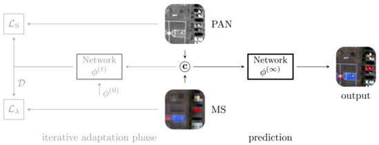
Figure 1.
Target-adaptive inference scheme Z-<Network Name>. Available for networks (A-)PNN, PanNet and DRPNN.
More in detail, said M and P are the MS and PAN input components, respectively, the pansharpened image and a suitable scaling operator. The overall loss is given by
where the two loss terms are weighted by to account for both spectral and spatial consistency. The spectral loss is given by
where indicates the -norm, and the low-resolution projection operator consists of band-dependent low-pass filtering, followed by spatial decimation at pace :
being a suitable band-dependent point spread function.
On the other hand, the spatial loss term is given by
where is the correlation coefficient computed in a window centered at location , between the b-th band of and P, and is an upper bound correlation field estimated on a smoothed version of P and the 23-tap polynomial interpolation of M. By doing so, image locations where the correlation coefficient between and P have reached the corresponding bounding level and do not contribute to the gradient computation. Experimental evidence suggested setting .
2.2. Proposed Fast CNN-Based Target-Adaptation Framework for Pansharpening
The core CNN architecture of Z-PNN is the model A-PNN summarized in Figure 2. It is relatively shallow in order to keep the computational overhead limited due to the adaptation phase (Figure 1). Nonetheless, such an overhead remains a serious issue that may prevent the use of this approach in critical situations when large-scale target images are concerned. As an example, on a commercial GPU, such as NVIDIA Quadro P6000, a 2048 × 2048 image (at PAN resolution) requires about a second per tuning iteration that sums up to a couple of minutes if hundred adaptation iterations are concerned. Such a timing scales about linearly with the image size as long as the GPU memory is capable at hosting the whole process, but once such capacity is exceeded, the computational burden grows much more quickly. Motivated by this consideration, we have explored a modified adaptation protocol still operating at full resolution and valid for generic pansharpening networks. The basic conjecture from which we have started is that the required adaptation is mainly due to the different atmospheric and geometrical conditions that can determine a mismatch between the training and the test datasets, whereas the intra-image spatial variability counts much less.
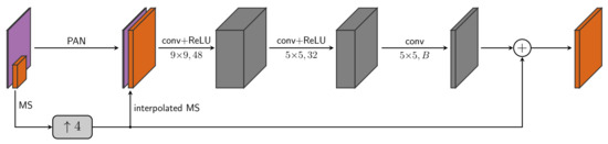
Figure 2.
A-PNN model for Z-PNN.
Atmospheric and/or geometrical mismatches between training and test datasets can occur easily. Fog, pollution and daylight conditions are typical examples of atmospheric parameters that can heavily impact image features such as contrast and intensity. Figure 3a shows two details of GeoEye-1 images with similar content (forest) but taken from different acquisitions. The two details show different contrast and brightness levels, mostly because of a different light condition. On the other hand, geometry (think of satellite viewing angle) also plays an important role. In fact, scenes acquired at Nadir present geometries that differ from those visible off-Nadir. Urban settlement orientations with respect to the satellite orbit can also have some relevance. Figure 3b shows another pair of crops, showing some buildings lying on WorldView-3 images acquired with different viewing angles. The buildings clearly show different skews. It goes without saying that data augmentation techniques can only partially address these kinds of data issues.
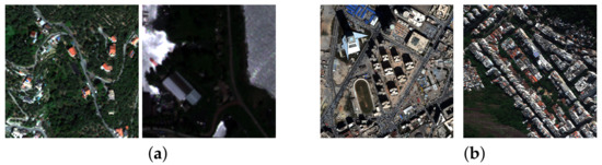
Figure 3.
Atmospheric (a) and geometrical (b) mismatch examples.
On the basis of the above considerations, it makes sense to run the tuning iterations on partial tiles of the target image. In particular, we start from a small (128 × 128) central crop of the image and run half of the prefixed total number of iterations (fixed to 256). Once this first burst of 128 iterations is completed, the crop size is doubled in each direction (keeping the central positioning), while a halved (64) number of iterations are queued to the tuning process. The process goes on with this rule until the current crop covers the whole image. Depending on the image size, a residual number of iterations are needed to reach the total number of 256 iterations. This residue, in case, can be completed on the crop corresponding to the whole image. This rule is summarized in Table 1.

Table 1.
Proposed target-adaptive iterations distribution. Bold numbers indicate the last phase (early stop) for the lighter version.
Besides this proposed method, hereinafter referred to as Fast Z-<Network Name>, we also test a lighter version, namely, Faster Z-<Network Name>, that undergoes an early stop of the tuning that allows skipping of the heaviest iterations that will involve the whole image (bold numbers in Table 1 correspond to the last tuning phase for the Faster version). In particular, for the sample network of Figure 2, the two versions will be called Fast Z-PNN and Faster Z-PNN, respectively. In addition to this, the “Z” versions of PanNet [25] and DRPNN [30], i.e., with full-resolution target-adaptation and loss (1), will also be tested.
3. Results
To prove the effectiveness of the proposed adaptation schedule, we carried out experiments on 2048 × 2048 WorldView-3, WorldView-2 and GeoEye1 images, parts of larger tiles covering the cities of Adelaide (courtesy of DigitalGlobe), Washington (courtesy of DigitalGlobe) and Genoa (courtesy of DigitalGlobe, provided by European Space Imaging), respectively. The image size (power of 2) simplifies the analysis of the proposed solution for obvious reasons but is by no means limiting in the validation of the basic idea. For each of the three cities/sensors, we disposed of four images—three for validation, the remaining for a test—as summarized in Table 2.
Table 2.
Datasets for validation and test. Adelaide and Washington, courtesy of DigitalGlobe. Genoa (DigitalGlobe) provided by ESA.
An RGB version of the MS component for each test image is shown in Figure 4, Figure 5 and Figure 6, respectively. Overlaid on the images are the crops involved in the several adaptation phases and some crops (A, B, C) that will be later recalled for the purpose of visual inspection of the results.
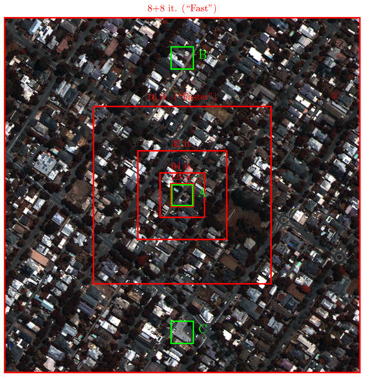
Figure 4.
MS (RGB version) component of the WorldView-3 test image of Adelaide. Red concentric squared boxes indicate the crops used during the adaptation phases (the smaller the box, the earlier the phase). Green boxes (A, B, C) highlight three crops selected for visual inspection purposes.
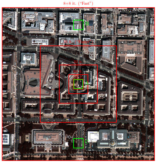
Figure 5.
MS (RGB version) component of the WorldView-2 test image of Washington. Red concentric squared boxes indicate the crops used during the adaptation phases (the smaller the box, the earlier the phase). Green boxes (A, B, C) highlight three crops selected for visual inspection purposes.
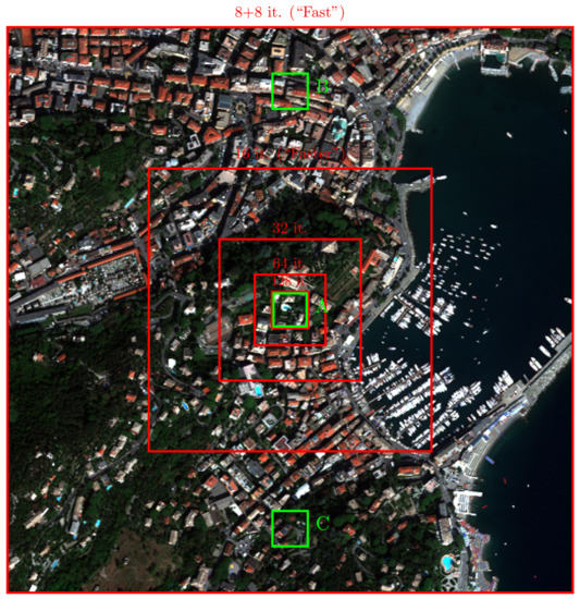
Figure 6.
MS (RGB version) component of the GeoEye-1 test image of Genoa. Red concentric squared boxes indicate the crops used during the adaptation phases (the smaller the box, the earlier the phase). Green boxes (A, B, C) highlight three crops selected for visual inspection purposes.
Table 3 summarizes the distribution of the number of iterations planned for each crop size and the corresponding computational time, by iteration and by phase. As it can be seen, the adaptation time for the proposed solution (see Fast Z-PNN on WV-∗ to fix the ideas) was about 12 s against 40 or 100 s for the baseline scheme when using 100 (default choice) or 256 iterations, respectively. Moreover, it is worth noticing that most of the time (6.42 s) was spent by the last iterations on the full image. Similar considerations apply for GeoEye-1, as well as for the other two models. In particular, notice that for Z-DRPNN, all time scores scaled since this model is heavier (more parameters) compared to Z-PNN and Z-PanNet.
Table 3.
Number of iterations for each image crop during the adaptation phase with corresponding unitary (Time/iter.) and cumulative (Time/phase) costs. The overall computational time for adaptation over WV-∗ /GE-1 images is about 12/6, 13/8 and 74/60 s for Z-PNN, Z-PanNet and Z-DRPNN, respectively, including an initial overhead of about a second for preliminary operations. Experiments have been run on a NVIDIA A100 GPU.
Actually, from a more careful inspection of Table 3, it can be noticed that the time per iteration tended to increase by a factor of 4, moving from one crop size to the next one when these were larger. In fact, Fast Z-PNN obtained the following time multipliers on WV-∗ : 1.17 (), 3.14, 3.51 and 3.84 (). This should not be surprising since the crop area increased by 4 when doubling its linear dimensions and also because the computational time on parallel computing units, such as GPUs, does not always scale linearly with the image size, particularly when the input images are relatively small or too large, causing memory swaps. Assuming to be in a linear regime where the iteration cost grows linearly with the image size (area), considering that the number of iterations halves from one phase to the next one, the time consumption per phase eventually doubled, moving from a phase to the next one. Asymptotically, each new phase took a time comparable to the time accumulated by all previous phases. Consequently, by skipping the last phase, one would save approximately half of the computational burden, paying something in terms of accuracy.
Based on the above considerations, we also tested the lighter configuration, “Faster”, of the proposed method, where we skipped the last tuning phase with an early stop, as indicated in Table 1.
The experimental evaluation was split in two parts. On one side, the proposed Fast and Faster variants were compared to the corresponding baselines (Z-∗) directly in terms of loss achieved during the target-adaptation phase. This was completed separately for both spectral and spatial loss components and using the validation images only. The results of this analysis for the whole validation dataset are summarized in Table 4 and Table 5, while Figure 7 displays the loss curves for a sample image. Moreover, Figure 8 compares the different target-adaptive schemes for Z-PNN using some sample visual results.
Table 4.
Run time for target-adaptation. and indicate the run time for Faster and Fast Z-PNN, who achieve the loss values and , respectively (: pretrained model). and are the run time for Z-PNN to reach the same loss levels achieved by its Faster and Fast versions, respectively. All times are given in seconds. In (a) is the WorldView-∗ case, in (b) GeoEye-1. Initialization time (about a second) fixed for all is not counted. Bold numbers indicate cases with non decreasing spatial loss.
Table 5.
Avarage run time for target-adaptation for all involved models, referred to the spectral losses.
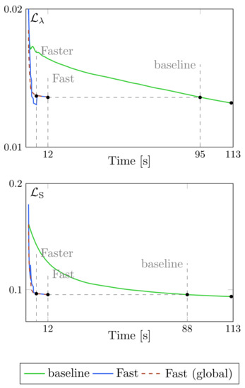
Figure 7.
Loss decay during the adaptation phase for Z-PNN on a sample WV-3 image: spectral (top) and spatial (bottom) loss terms. The loss of the baseline model is shown in green; the loss of the proposed solution (computed on the current crop) is shown in blue; dashed red lines show the loss of the proposed model during training computed on the whole image.
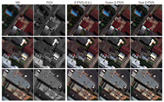
Figure 8.
Pansharpening results without adaptation (0 it.), with partial (Faster) and full (Fast) adaptation according to the proposed scheme. From top to bottom: WV-3 Adelaide crops A, B and C, respectively.
On the other hand, the test images were used for a comparative quality assessment in terms of both pansharpening numerical indexes and subjective visual inspection. For a more robust quality evaluation, we resorted to the pansharpening benchmark toolbox [11], which provides the implementation of several state-of-the-art methods and several quality indexes, e.g., the spectral and spatial consistency indexes. We integrated the benchmark with the Machine Learning toolbox proposed in [39], which provides additional CNN-based methods. Furthermore, the evaluation was carried out using the additional indexes , R-SAM, R-ERGAS and R-, recently proposed in [40]. All comparative methods are summarized in Table 6. The results are gathered in Table 7, Table 8 and Table 9, whereas sample visual results are given in Figure 9, Figure 10 and Figure 11. A deeper discussion about these results is left to Section 4.
Table 6.
Detailed list of all reference methods.
Table 7.
Numerical results on the 2048 × 2048 WorldView-3 test image (Adelaide), courtesy of DigitalGlobe.
Table 8.
Numerical results on the 2048 × 2048 WorldView-2 test image (Washington), courtesy of DigitalGlobe.
Table 9.
Numerical results on the 2048 × 2048 GeoEye-1 test image (Genoa), DigitalGlobe, Inc. (2018), provided by European Space Agency.
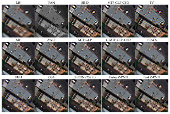
Figure 9.
Pansharpening results on the WorldView-3 Adelaide image (crop C).
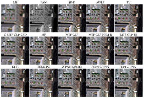
Figure 10.
Pansharpening results on the WorldView-2 Washington image (crop B).
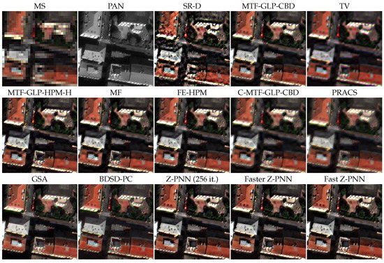
Figure 11.
Pansharpening results on the GeoEye-1 Washington image (crop B).
4. Discussion
Let us now analyze in depth the provided results, starting from a comparison with the baseline models Z-∗.
In Figure 7, we show the loss decay during the adaptation phase, separately for the spectral (top) and spatial (bottom) terms, as a function of the running time rather than the iteration count. This experiment refers to a WorldView-3 image processed by Z-PNN models, but similar behaviors have been observed for the other images, regardless of the employed base model. The loss terms for the baseline (Z-PNN) and the proposed Fast Z-PNN are plotted in green and blue, respectively. Although the loss is a per-pixel loss (spatial average), so that these curves are dimensionally consistent, the latter refers to the current crop while the former is an average on the whole image. For this reason, for the proposed (Fast/Faster) solution, we also computed the value of the loss on the whole image at each iteration (red dashed line). Surprisingly, the “global” loss tightly follows the “local” (to crop) loss, showing a more regular decay, thanks to a wider average. These plots clearly show the considerable computational gain achievable for any fixed target loss level. It is worth noticing, for example, that the loss levels achieved by the proposed Fast scheme in 12 s (256 iterations) are reached by the baseline approach in about 90 s (∼200 iterations on the full image). Besides, the Faster version reaches almost the same loss levels of the Fast version in about 5.7 s.
In Table 4, for each validation image, we quantify the computational gains achieved by Faster and Fast Z-PNN in terms of time consumption. For each image, it is indicated, separately for the spectral (top table) and spatial (bottom table) loss components, the value without adaptation () and those achieved by Faster () and Fast () adaptation schemes (these values refer to the loss assessed on the whole image, not to the one computed on the crops for gradient descent), whose run times ( and ) do not depend on the specific image (they drop when working with GeoEye-1 instead of WV-∗ because of the smaller number of spectral bands). Then, we report the times and needed for Z-PNN to reach the loss levels and , respectively. We can fairly read and as the times needed for Z-PNN to achieve the same spectral (top table) or spatial (bottom table) target levels of its faster versions. Consequently, and represent the computational gains of the proposed solution. Similar results, not shown for brevity, have been registered for Z-PanNet and Z-DRPNN. It is worth noticing that whereas for the spectral loss the gain is always (well) larger than 1, for the spatial component, there can occur cases where it is already pretty low (see in Table 4); hence, only the spectral loss decays while the spatial one either keeps constant or even grows a little (see bold numbers in Table 4). In these cases, the gains cannot be computed, but actually, it make sense to focus on the spectral behavior only, as no adaptation is needed on the spatial side.
In general, from all experiments that we carried out, it emerges that the adaptation is mostly needed for the reduction of the spectral distortion rather than for the spatial one. This is a particular feature of the Z-∗ framework, which leverages a spatial consistency loss based on correlation (Equation (4)) that shows a quite robust behavior. On the basis of the above reasons, it makes sense to focus on the spectral loss only for checking the quality alignment between Z-∗ and the proposed variants. Therefore, we can give a look to Table 5, which provides the average gains for all models, averaged by sensor, but limited to the spectral part. Overall, it can be observed that the Fast models allow for obtaining gains ranging from 4.03 to 15.6 (9.6 on average), whereas Faster models provide gains between 6.33 to 26.8 (17.9 on average), at the price of a little increase of the loss components (compare the loss levels in Table 4).
Let us now move to the analysis of the results obtained on the test images for a comparison with the state-of-the-art solutions. Starting from the numerical results gathered in Table 7 (WV-3), Table 8 (WV-2) and Table 9 (GE-1), we can observe that the most important achievement is that the proposed Faster and Fast solutions are exactly where they are expected to be, i.e., between Z-∗ (100 it.) and Z-∗ (256 it.) almost always, coherently with the loss levels shown in Figure 7 and Table 4, with few exceptions. In some cases, the proposals behave even better than the baseline (e.g., Fast-Z-PNN against Z-PNN on GeoEye-1, Table 9). Moreover, it is worth noticing that Faster Z-∗ tightly follows Fast Z-∗ and Z-∗ (256 it.), confirming our initial guess that the need for tuning is mostly due to geometric or atmospheric misalignments between the training and testing datasets rather than grounding content mismatches.
Concerning the overall comparison, it must be underlined that all indexes are used on the full-resolution image without any ground-truth. They assess the consistency rather than the synthesis properties, and each reflects some arbitrary assumption. Both and deal with the spatial consistency, while the remaining relate to the spectral consistency. While the latter group shows a good level of agreement, the former looks much less correlated. For a deeper discussion on this issue that is a little out of scope here, the Reader is referred to [35]. In addition, the goal of the present contribution is on efficiency rather than on accuracy; therefore, we leave these results to the reader without further discussion.
Beside numerical assessment, the visual inspection of the results is a fundamental complementary check to gain insight into the behavior of the compared methods. Let us first analyze the impact of the tuning phase by comparing the pretrained model Z-∗ (0 it.) with the proposed target-adaptive solutions, Faster and Fast versions. Figure 8 shows a few crops from WV-3 Adelaide image (Figure 4), with the related pansharpened images obtained with the Z-PNN variants. Remarkable differences can be noticed between the pretrained model and the two target-adaptive options. The Reader may notice the visible artifacts introduced by the pretrained model occurring, for example, in the pool of crop A or on several building roofs (spotted artifacts), which are removed by the proposed solutions, thanks to the tuning. On the other hand, there is no noticeable difference between the Faster and Fast configurations proposed. It is also worth noticing that this alignment between the Fast and the Faster configurations hold indistinguishably on crop A (always involved in the tuning) and crops B and C that are not involved in the tuning process in the Faster version (see Figure 4). Similar considerations can be noted from the experiments, not shown for brevity, carried out on the other datasets and/or using different baseline models.
Figure 9, Figure 10 and Figure 11 show, again, on some selected crops, the pansharpening results obtained by the proposed solutions and by the best performing ones among all comparative methods listed in Table 6 for the WorldView-3, WorldView-2 and GeoEye-1 images, respectively. In particular, these results confirm the most relevant observation that Fast Z-PNN, Faster Z-PNN and the baseline Z-PNN are nearly indistinguishable, in line with the numerical results discussed above, further underlining that the registered computational gain has been achieved without sacrificing accuracy. Regarding the comparison with the other methods, from the visual point of view, the proposed solutions are aligned with the best ones, without appreciable spectral or spatial distortion and a very high contrast level.
Finally, in order to further prove the robustness of the proposed approach, we ran a cross-image experiment. Taking two different WV-3 sample images whose content is sufficiently different (see Figure 12), we ran Fast Z-PNN on the first one (a), which plays as a target image. On the same image, we also tested Z-PNN without adaptation (0 it.) and the model adapted on image (b) using the Fast configuration. The numerical results, shown in (c), provide further confirmation that the actual content of the image has a minor impact on pansharpening, in the tuning phase, with respect to acquisition geometry and atmospheric conditions.
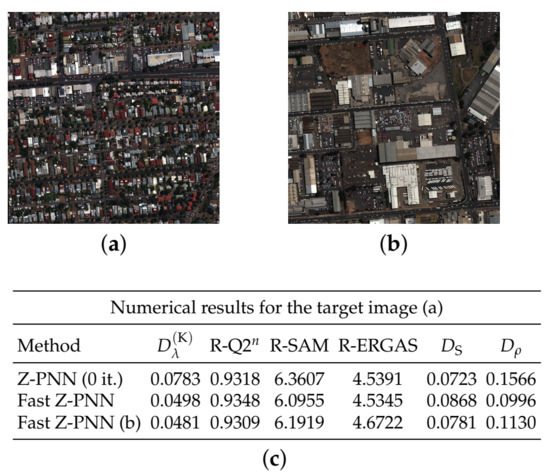
Figure 12.
Cross-image adaptation test. (a) target image; (b) a different image from the same validation dataset (WV-3); (c) numerical results. Fast Z-PNN (b) corresponds to the results on (a) with the model fitted on (b).
5. Conclusions
In this work, we have presented a new target-adaptive framework for CNN pansharpening. A full-version named Fast and a quicker configuration named Faster have been tested over the recently proposed unsupervised full-resolution models: Z-PNN, Z-PanNet and Z-DRPNN [35]. The results clearly show that the inference time reduces by a factor of 10 or more, which doubles for the Faster version, without sacrificing accuracy. Such gain has been achieved thanks to the assumption, experimentally validated here, that generalization problems occur when training and test datasets come from different acquisitions, hence because of geometrical and/or atmospheric changes, whereas different areas of a same image can be considered sufficiently “homogeneous” from the learning point of view. Starting from this consideration, the proposed target adaptive scheme does not make use of the full test image for its unsupervised adaptation from the beginning, but, starting from a central portion, it progressively encloses all data in the process. Indeed, the Faster version only uses 25% of the image, obtaining nearly the same quality level.
Future work may explore different spatial sampling strategies, such as adaptive or dynamic selection of the tuning crops, in order to further improve the robustness and generality of the proposed framework.
Author Contributions
Conceptualization, G.S. and M.C.; methodology, G.S. and M.C.; software, M.C.; validation, G.S. and M.C.; formal analysis, G.S. and M.C.; investigation, G.S. and M.C.; resources, G.S. and M.C.; data curation, M.C.; writing—original draft preparation, G.S.; writing—review and editing, G.S. and M.C.; visualization, M.C.; supervision, G.S. All authors have read and agreed to the published version of the manuscript.
Funding
This research received no external funding.
Data Availability Statement
Not applicable.
Acknowledgments
The authors would like to thank DigitalGlobe and ESA for providing sample images for research purposes.
Conflicts of Interest
The authors declare no conflict of interest.
References
- Moser, G.; Serpico, S. Generalized minimum-error thresholding for unsupervised change detection from SAR amplitude imagery. IEEE Trans. Geosci. Remote Sens. 2006, 44, 2972–2982. [Google Scholar] [CrossRef]
- Chen, Y.; Bruzzone, L. Self-Supervised SAR-Optical Data Fusion of Sentinel-1/-2 Images. IEEE Trans. Geosci. Remote Sens. 2022, 60, 5406011. [Google Scholar] [CrossRef]
- Errico, A.; Angelino, C.V.; Cicala, L.; Podobinski, D.P.; Persechino, G.; Ferrara, C.; Lega, M.; Vallario, A.; Parente, C.; Masi, G.; et al. SAR/multispectral image fusion for the detection of environmental hazards with a GIS. In Proceedings of the SPIE—The International Society for Optical Engineering, Amsterdam, The Netherlands, 22–25 September 2014; Volume 9245. [Google Scholar]
- Scarpa, G.; Gargiulo, M.; Mazza, A.; Gaetano, R. A CNN-Based Fusion Method for Feature Extraction from Sentinel Data. Remote Sens. 2018, 10, 236. [Google Scholar] [CrossRef]
- Vivone, G.; Alparone, L.; Chanussot, J.; Mura, M.D.; Garzelli, A.; Licciardi, G.A.; Restaino, R.; Wald, L. A Critical Comparison Among Pansharpening Algorithms. IEEE Trans. Geosci. Remote Sens. 2015, 53, 2565–2586. [Google Scholar] [CrossRef]
- Gargiulo, M.; Mazza, A.; Gaetano, R.; Ruello, G.; Scarpa, G. A CNN-Based Fusion Method for Super-Resolution of Sentinel-2 Data. In Proceedings of the IGARSS 2018–2018 IEEE International Geoscience and Remote Sensing Symposium, Valencia, Spain, 22–27 July 2018; pp. 4713–4716. [Google Scholar] [CrossRef]
- Ciotola, M.; Ragosta, M.; Poggi, G.; Scarpa, G. A full-resolution training framework for Sentinel-2 image fusion. In Proceedings of the IGARSS 2021, Brussels, Belgium, 11–16 July 2021; pp. 1–4. [Google Scholar]
- Ciotola, M.; Martinelli, A.; Mazza, A.; Scarpa, G. An Adversarial Training Framework for Sentinel-2 Image Super-Resolution. In Proceedings of the IGARSS 2022—2022 IEEE International Geoscience and Remote Sensing Symposium, Kuala Lumpur, Malaysia, 17–22 July 2022; pp. 3782–3785. [Google Scholar] [CrossRef]
- Peng, D.; Bruzzone, L.; Zhang, Y.; Guan, H.; Ding, H.; Huang, X. SemiCDNet: A Semisupervised Convolutional Neural Network for Change Detection in High Resolution Remote-Sensing Images. IEEE Trans. Geosci. Remote Sens. 2021, 59, 5891–5906. [Google Scholar] [CrossRef]
- Gaetano, R.; Amitrano, D.; Masi, G.; Poggi, G.; Ruello, G.; Verdoliva, L.; Scarpa, G. Exploration of multitemporal COSMO-skymed data via interactive tree-structured MRF segmentation. IEEE J. Sel. Top. Appl. Earth Obs. Remote Sens. 2014, 7, 2763–2775. [Google Scholar] [CrossRef]
- Vivone, G.; Dalla Mura, M.; Garzelli, A.; Restaino, R.; Scarpa, G.; Ulfarsson, M.O.; Alparone, L.; Chanussot, J. A New Benchmark Based on Recent Advances in Multispectral Pansharpening: Revisiting Pansharpening With Classical and Emerging Pansharpening Methods. IEEE Geosci. Remote Sens. Mag. 2021, 9, 53–81. [Google Scholar] [CrossRef]
- Chavez, P.S.; Kwarteng, A.W. Extracting spectral contrast in Landsat thematic mapper image data using selective principal component analysis. Photogramm. Eng. Remote Sens. 1989, 55, 339–348. [Google Scholar]
- Tu, T.M.; Huang, P.S.; Hung, C.L.; Chang, C.P. A fast intensity hue-saturation fusion technique with spectral adjustment for IKONOS imagery. IEEE Geosci. Remote Sens. Lett. 2004, 1, 309–312. [Google Scholar] [CrossRef]
- Gillespie, A.R.; Kahle, A.B.; Walker, R.E. Color enhancement of highly correlated images. II. Channel ratio and “chromaticity” transformation techniques. Remote Sens. Environ. 1987, 22, 343–365. [Google Scholar] [CrossRef]
- Laben, C.A.; Brower, B.V. Process for Enhancing the Spatial Resolution of Multispectral Imagery Using Pan-Sharpening. U.S. Patent 6011875, 4 January 2000. [Google Scholar]
- Ranchin, T.; Wald, L. Fusion of high spatial and spectral resolution images: The ARSIS concept and its implementation. Photogramm. Eng. Remote Sens. 2000, 66, 49–61. [Google Scholar]
- Aiazzi, B.; Alparone, L.; Baronti, S.; Garzelli, A. Context-driven fusion of high spatial and spectral resolution images based on oversampled multiresolution analysis. IEEE Trans. Geosci. Remote Sens. 2002, 40, 2300–2312. [Google Scholar] [CrossRef]
- Khan, M.M.; Chanussot, J.; Condat, L.; Montanvert, A. Indusion: Fusion of Multispectral and Panchromatic Images Using the Induction Scaling Technique. IEEE Geosci. Remote Sens. Lett. 2008, 5, 98–102. [Google Scholar] [CrossRef]
- Restaino, R.; Mura, M.D.; Vivone, G.; Chanussot, J. Context-Adaptive Pansharpening Based on Image Segmentation. IEEE Trans. Geosci. Remote Sens. 2017, 55, 753–766. [Google Scholar] [CrossRef]
- Palsson, F.; Sveinsson, J.R.; Ulfarsson, M.O. A New Pansharpening Algorithm Based on Total Variation. Geosci. Remote Sens. Lett. IEEE 2014, 11, 318–322. [Google Scholar] [CrossRef]
- Palsson, F.; Sveinsson, J.R.; Ulfarsson, M.O.; Benediktsson, J.A. Model-Based Fusion of Multi- and Hyperspectral Images Using PCA and Wavelets. IEEE Trans. Geosci. Remote Sens. 2015, 53, 2652–2663. [Google Scholar] [CrossRef]
- Vivone, G.; Simões, M.; Dalla Mura, M.; Restaino, R.; Bioucas-Dias, J.M.; Licciardi, G.A.; Chanussot, J. Pansharpening Based on Semiblind Deconvolution. IEEE Trans. Geosci. Remote Sens. 2015, 53, 1997–2010. [Google Scholar] [CrossRef]
- Palsson, F.; Ulfarsson, M.O.; Sveinsson, J.R. Model-Based Reduced-Rank Pansharpening. IEEE Geosci. Remote Sens. Lett. 2020, 17, 656–660. [Google Scholar] [CrossRef]
- Masi, G.; Cozzolino, D.; Verdoliva, L.; Scarpa, G. Pansharpening by Convolutional Neural Networks. Remote Sens. 2016, 8, 594. [Google Scholar] [CrossRef]
- Yang, J.; Fu, X.; Hu, Y.; Huang, Y.; Ding, X.; Paisley, J. PanNet: A Deep Network Architecture for Pan-Sharpening. In Proceedings of the ICCV, Venice, Italy, 22–29 October 2017. [Google Scholar] [CrossRef]
- Masi, G.; Cozzolino, D.; Verdoliva, L.; Scarpa, G. CNN-based Pansharpening of Multi-Resolution Remote-Sensing Images. In Proceedings of the Joint Urban Remote Sensing Event, Dubai, United Arab Emirates, 6–8 March 2017. [Google Scholar]
- Yuan, Q.; Wei, Y.; Meng, X.; Shen, H.; Zhang, L. A Multiscale and Multidepth Convolutional Neural Network for Remote Sensing Imagery Pan-Sharpening. IEEE J. Sel. Top. Appl. Earth Obs. Remote Sens. 2018, 11, 978–989. [Google Scholar] [CrossRef]
- Shao, Z.; Cai, J. Remote Sensing Image Fusion With Deep Convolutional Neural Network. IEEE J. Sel. Topics Appl. Earth Observ. 2018, 11, 1656–1669. [Google Scholar] [CrossRef]
- Vicinanza, M.R.; Restaino, R.; Vivone, G.; Mura, M.D.; Chanussot, J. A Pansharpening Method Based on the Sparse Representation of Injected Details. IEEE Geosci. Remote Sens. Lett. 2015, 12, 180–184. [Google Scholar] [CrossRef]
- Wei, Y.; Yuan, Q.; Shen, H.; Zhang, L. Boosting the Accuracy of Multispectral Image Pansharpening by Learning a Deep Residual Network. IEEE Geosci. Remote Sens. Lett. 2017, 14, 1795–1799. [Google Scholar] [CrossRef]
- Luo, S.; Zhou, S.; Feng, Y.; Xie, J. Pansharpening via Unsupervised Convolutional Neural Networks. IEEE J. Sel. Top. Appl. Earth Obs. Remote Sens. 2020, 13, 4295–4310. [Google Scholar] [CrossRef]
- Seo, S.; Choi, J.S.; Lee, J.; Kim, H.H.; Seo, D.; Jeong, J.; Kim, M. UPSNet: Unsupervised Pan-Sharpening Network With Registration Learning Between Panchromatic and Multi-Spectral Images. IEEE Access 2020, 8, 201199–201217. [Google Scholar] [CrossRef]
- Wald, L.; Ranchin, T.; Mangolini, M. Fusion of satellite images of different spatial resolution: Assessing the quality of resulting images. Photogramm. Eng. Remote Sens. 1997, 63, 691–699. [Google Scholar]
- Vitale, S.; Scarpa, G. A Detail-Preserving Cross-Scale Learning Strategy for CNN-Based Pansharpening. Remote Sens. 2020, 12, 348. [Google Scholar] [CrossRef]
- Ciotola, M.; Vitale, S.; Mazza, A.; Poggi, G.; Scarpa, G. Pansharpening by convolutional neural networks in the full resolution framework. IEEE Trans. Geosci. Remote Sens. 2022, 60, 5408717. [Google Scholar] [CrossRef]
- Scarpa, G.; Vitale, S.; Cozzolino, D. Target-Adaptive CNN-Based Pansharpening. IEEE Trans. Geosci. Remote. Sens. 2018, 56, 5443–5457. [Google Scholar] [CrossRef]
- Zhang, Y.; Liu, C.; Sun, M.; Ou, Y. Pan-Sharpening Using an Efficient Bidirectional Pyramid Network. IEEE Trans. Geosci. Remote Sens. 2019, 57, 5549–5563. [Google Scholar] [CrossRef]
- Xu, S.; Zhang, J.; Zhao, Z.; Sun, K.; Liu, J.; Zhang, C. Deep Gradient Projection Networks for Pan-sharpening. In Proceedings of the 2021 IEEE/CVF Conference on Computer Vision and Pattern Recognition (CVPR), Nashville, TN, USA, 20–25 June 2021; pp. 1366–1375. [Google Scholar] [CrossRef]
- Deng, L.J.; Vivone, G.; Paoletti, M.E.; Scarpa, G.; He, J.; Zhang, Y.; Chanussot, J.; Plaza, A.J. Machine Learning in Pansharpening: A Benchmark, from Shallow to Deep Networks. IEEE Geosci. Remote Sens. Mag. 2022, 10, 279–315. [Google Scholar] [CrossRef]
- Scarpa, G.; Ciotola, M. Full-Resolution Quality Assessment for Pansharpening. Remote Sens. 2022, 14, 1808. [Google Scholar] [CrossRef]
- Lolli, S.; Alparone, L.; Garzelli, A.; Vivone, G. Haze Correction for Contrast-Based Multispectral Pansharpening. IEEE Geosci. Remote Sens. Lett. 2017, 14, 2255–2259. [Google Scholar] [CrossRef]
- Garzelli, A.; Nencini, F.; Capobianco, L. Optimal MMSE pan sharpening of very high resolution multispectral images. IEEE Trans. Geosci. Remote Sens. 2008, 46, 228–236. [Google Scholar] [CrossRef]
- Garzelli, A. Pansharpening of Multispectral Images Based on Nonlocal Parameter Optimization. IEEE Trans. Geosci. Remote Sens. 2015, 53, 2096–2107. [Google Scholar] [CrossRef]
- Vivone, G. Robust Band-Dependent Spatial-Detail Approaches for Panchromatic Sharpening. IEEE Trans. Geosci. Remote Sens. 2019, 57, 6421–6433. [Google Scholar] [CrossRef]
- Aiazzi, B.; Baronti, S.; Selva, M. Improving component substitution pansharpening through multivariate regression of MS+Pan data. IEEE Trans. Geosci. Remote Sens. 2007, 45, 3230–3239. [Google Scholar] [CrossRef]
- Choi, J.; Yu, K.; Kim, Y. A New Adaptive Component-Substitution-Based Satellite Image Fusion by Using Partial Replacement. IEEE Trans. Geosci. Remote Sens. 2011, 49, 295–309. [Google Scholar] [CrossRef]
- Otazu, X.; Gonzalez-Audicana, M.; Fors, O.; Nunez, J. Introduction of sensor spectral response into image fusion methods. Application to wavelet-based methods. IEEE Trans. Geosci. Remote Sens. 2005, 43, 2376–2385. [Google Scholar] [CrossRef]
- Alparone, L.; Garzelli, A.; Vivone, G. Intersensor Statistical Matching for Pansharpening: Theoretical Issues and Practical Solutions. IEEE Trans. Geosci. Remote Sens. 2017, 55, 4682–4695. [Google Scholar] [CrossRef]
- Vivone, G.; Restaino, R.; Chanussot, J. Full Scale Regression-Based Injection Coefficients for Panchromatic Sharpening. IEEE Trans. Image Process. 2018, 27, 3418–3431. [Google Scholar] [CrossRef] [PubMed]
- Vivone, G.; Restaino, R.; Chanussot, J. A Regression-Based High-Pass Modulation Pansharpening Approach. IEEE Trans. Geosci. Remote Sens. 2018, 56, 984–996. [Google Scholar] [CrossRef]
- Alparone, L.; Wald, L.; Chanussot, J.; Thomas, C.; Gamba, P.; Bruce, L. Comparison of pansharpening algorithms: Outcome of the 2006 GRS-S Data-Fusion Contest. IEEE Trans. Geosci. Remote Sens. 2007, 45, 3012–3021. [Google Scholar] [CrossRef]
- Restaino, R.; Vivone, G.; Dalla Mura, M.; Chanussot, J. Fusion of Multispectral and Panchromatic Images Based on Morphological Operators. IEEE Trans. Image Process. 2016, 25, 2882–2895. [Google Scholar] [CrossRef]
- He, L.; Rao, Y.; Li, J.; Chanussot, J.; Plaza, A.; Zhu, J.; Li, B. Pansharpening via detail injection based convolutional neural networks. IEEE J. Sel. Top. Appl. Earth Obs. Remote Sens. 2019, 12, 1188–1204. [Google Scholar] [CrossRef]
- Deng, L.J.; Vivone, G.; Jin, C.; Chanussot, J. Detail injection-based deep convolutional neural networks for pansharpening. IEEE Trans. Geosci. Remote. Sens. 2020, 59, 6995–7010. [Google Scholar] [CrossRef]


Disclaimer/Publisher’s Note: The statements, opinions and data contained in all publications are solely those of the individual author(s) and contributor(s) and not of MDPI and/or the editor(s). MDPI and/or the editor(s) disclaim responsibility for any injury to people or property resulting from any ideas, methods, instructions or products referred to in the content. |
© 2023 by the authors. Licensee MDPI, Basel, Switzerland. This article is an open access article distributed under the terms and conditions of the Creative Commons Attribution (CC BY) license (https://creativecommons.org/licenses/by/4.0/).