Strip Attention Networks for Road Extraction

Abstract

In recent years, deep learning methods have been widely used for road extraction in remote sensing images. However, the existing deep learning semantic segmentation networks generally show poor continuity in road segmentation due to the high-class similarity between roads and buildings surrounding roads in remote sensing images, and the existence of shadows and occlusion. To deal with this problem, this paper proposes strip attention networks (SANet) for extracting roads in remote sensing images. Firstly, a strip attention module (SAM) is designed to extract the contextual information and spatial position information of the roads. Secondly, a channel attention fusion module (CAF) is designed to fuse low-level features and high-level features. The network is trained and tested using the CITY-OSM dataset, DeepGlobe road extraction dataset, and CHN6-CUG dataset. The test results indicate that SANet exhibits excellent road segmentation performance and can better solve the problem of poor road segmentation continuity compared with other networks.

1. Introduction

Recently, with the development of computer technology and satellite technology, road extraction from remote sensing images has become more common. Remote sensing image road extraction has a wide range of applications, such as vehicle navigation, urban planning, intelligent transportation, image registration, geographic information system updates, and land use detection. The accuracy of road extraction is not only related to the extraction of vehicles, buildings, and other ground objects, but also one of the key technologies in research fields such as natural disaster early warning, military strikes, and unmanned vehicle path planning [1]. Meanwhile, remote sensing image road segmentation has its uniqueness and difficulty compared with general segmentation tasks [2,3,4].

The extraction of roads using segmentation algorithms is performed based on the development of computer vision image segmentation techniques, and image segmentation methods can be broadly classified into traditional algorithms and deep learning algorithms. Traditional algorithms mainly include the Gabor filter [5], Sobel operator [6], and watershed algorithm [7], as well as more advanced machine learning methods such as Support Vector Machine (SVM) [8] and Random Forests (RF) [9]. These methods perform image segmentation by extracting features, such as textures, edges, shapes, etc., from remote sensing images to achieve target extraction. For example, the Snake algorithm proposed by Kass et al. [10] and the method proposed by Shi et al. [11] both identify roads through spectral features and shape features. Ghaziani [12] proposes a method to extract roads using binary image segmentation. Unsalan [13] uses edge detection and a voting mechanism for road extraction. These methods rely heavily on the quality of the extracted features. However, in remote sensing images, roads are represented as narrow lines with connectivity, and some lines will cover the whole image and multiple roads may have cross-connections [14]. The features to be extracted are complex and rich, and there are many interferences, so traditional image segmentation methods are difficult to use for road extraction. In recent years, deep learning techniques have developed rapidly in the field of computer vision research, and deep learning methods automatically acquire non-linear and hierarchical features of images [15], which can better solve the problems existing in road extraction. Semantic segmentation is the main research direction of deep learning in the field of image segmentation, which can more comprehensively use convolutional neural networks (CNNs) [16] to extract low-level and high-level features of images from input images, with high segmentation accuracy and efficiency.

In recent years, many scholars have proposed some deep learning research methods for high-resolution road image extraction, but these methods still face difficulties such as high inter-class similarity, noisy interference, and the difficult extraction of narrow roads [17]. In 2014, Long et al. proposed fully convolutional networks (FCN) [18]. The FCN replaces the last fully connected layer of the CNN with a deconvolution, which is used to upsample the feature map of the last convolution layer so that it can return to the same dimensions as the input image. The spatial information is preserved while predicting each pixel. It can be applied to input images of arbitrary size and allows the network to ensure both robustness and accuracy. However, FCN cannot fully extract contextual information and the semantic segmentation accuracy is poor. In 2015, Ronneberger et al. proposed an improved U-Net [19] based on FCN with an encoder–decoder network structure. It can maintain a certain segmentation accuracy when the training set samples are small. In the same year, He et al. proposed deep residual networks (ResNet) [20], which avoid the problems of model overfitting, gradient disappearance, and gradient explosion caused by increasing the network depth. Zhang et al. [21] proposed a new model to combine UNet with ResNet to reduce the number of parameters required for training, making the network easier to train and making the road extraction results more accurate. In 2017, Zhao et al. proposed the pyramid scene parsing network (PSPNet) [22], which uses a pyramid pooling module; in 2018, Chen et al. proposed the DeeplabV3+ network [23], which uses atrous spatial pyramid pooling (ASPP), both of which extract multi-scale semantic information and fuse them to improve segmentation accuracy. Zhou et al. [24] modified the structure of LinkNet [25] by adding a special cavity convolution module to its central part, enabling the network to learn multi-scale features of roads. However, they focus only on macroscopic spatial position information and pay insufficient attention to detailed aspects.

The attention mechanism gives the neural network the ability to focus on certain focused parts of the input image. In 2017, Hu et al. proposed squeeze-and-excitation networks (SE-Net) [26] by adding the channel attention mechanism to the backbone. In 2018, Woo et al. proposed the convolutional block attention module (CBAM) [27] by adding global maximum pooling to the SE module and introducing the spatial attention mechanism. In the same year, dual attention network (DANet) [28] proposed by Fu et al. used two types of attention modules to model semantic interdependencies in spatial and channel dimensions. In 2020, Yu et al. proposed a context prior for scene segmentation (CPNet) [29], which selectively aggregates inter and intra-class information to realize segmentation of difficult samples.

Although existing semantic segmentation networks have achieved certain results, using these methods for segmenting roads often fails to achieve good results. Therefore, in this paper, we propose a SANet. When the roads segmented by other networks are interrupted, the method proposed in this paper can extract the roads more clearly and ensure the connectivity of the roads. The main contributions of this paper are drawn as follows:

• A novel encoder–decoder network has been designed and a SAM is proposed for extracting road features in row direction and column direction in images;
• A novel CAF is designed to extract the position information of roads in the low-level feature map and the category information in the high-level feature map, and to fuse them efficiently.

The source code is available at: https://github.com/YuShengC308/Strip-Attention-Net, accessed on 30 August 2022.

2. Materials and Methods

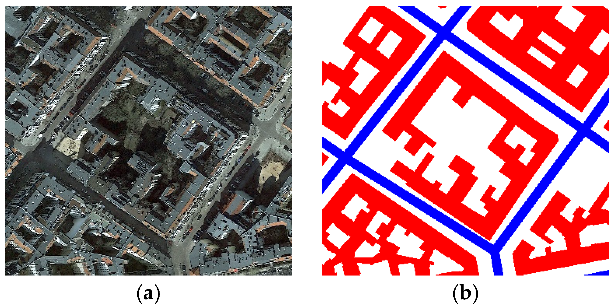
2.1. Datasets

The experiments in this paper are mainly based on three publicly available datasets. The first dataset is the CITY-OSM dataset [30], with a total of 825 images of 2611×2453 pixels each. The images were randomly selected in a ratio of 4:1, of which 660 images were used as the training set and the remaining 165 images were used as the test set. The test set’s true-color images and labeled maps are shown in Figure 1. The dataset has three categories, namely, background, buildings, and roads.

The second dataset is the DeepGlobe road extraction remote sensing map dataset, which has 6226 remote sensing images. Each image size is 1500 × 1500 pixels, randomly selected according to the ratio of 4:1, and 4981 images were used as the training set and the remaining 1245 images were used as test set. The test set’s true-color images and labeled maps are shown in Figure 2. The dataset has two categories, road and background categories. The DeepGlobe road extraction dataset is publicly available at https://competitions.codalab.org/competitions/18467, accessed on 18 June 2018.

The third dataset is the CHN6-CUG dataset [31]. CHN6-CUG contains 4511 labeled images of 512 × 512 size, divided into 3608 instances for the training set and 903 for the test set. The test set’s true-color images and labeled maps are shown in Figure 3. The CHN6-CUG road dataset is a new large-scale satellite image dataset of representative cities in China. Its remote sensing image base map is from Google Earth. Six cities with different levels of urbanization, city size, development degree, urban structure, and history and culture are selected, including the Chaoyang area of Beijing, the Yangpu District of Shanghai, Wuhan city center, the Nanshan area of Shenzhen, the Shatin area of Hong Kong, and Macao. A marked road consists of both covered and uncovered roads, depending on the degree of road coverage. According to the physical point of view of geographical factors, marked roads include railways, highways, urban roads, and rural roads, etc. The dataset has two categories, the first category is roads and all the remaining scenes are background categories.

2.2. Experimental Environment

The experiments are done under the Pytorch framework on Centos 7.8 with an Intel I9-9900KF CPU, 64-GB memory and two NVIDIA 2080Ti graphics cards with 11GB video memory as the hardware of the experimental platform. In this paper, we use the Mmsegmentation [32] semantic segmentation open source toolkit. The learning decay strategy is Poly learning rate decay strategy, the initial learning rate is 0.01, the minimum learning rate is 0.0004, the loss function is cross entropy, the optimizer is Stochastic gradient descent (SGD).

2.3. Evaluation Metrics

To evaluate the performance of segmentation, confusion matrix-based evaluation metrics were used: mean intersection over union (MIoU), which is an important general metric for image segmentation accuracy in the field of semantic segmentation. It is calculated by first calculating the intersection over union (IoU) for each category, and then dividing the sum of the intersection ratios of all categories by the number of categories. This process can be defined as follows:

$$\mathrm{IoU}=\frac{\mathit{TP}}{\mathit{TP}+\mathit{FP}+\mathit{FN}}$$

(1)

$$\mathrm{MIoU}=\frac{1}{n}{\displaystyle \sum }_{i=1}^n\frac{\mathit{TP}}{\mathit{TP}+\mathit{FP}+\mathit{FN}}$$

(2)

where TP is the positive category that is classified accurately, FP is the negative category that is misclassified as positive, TN is the negative category that is classified accurately, and FN is the positive category that is misclassified as negative.

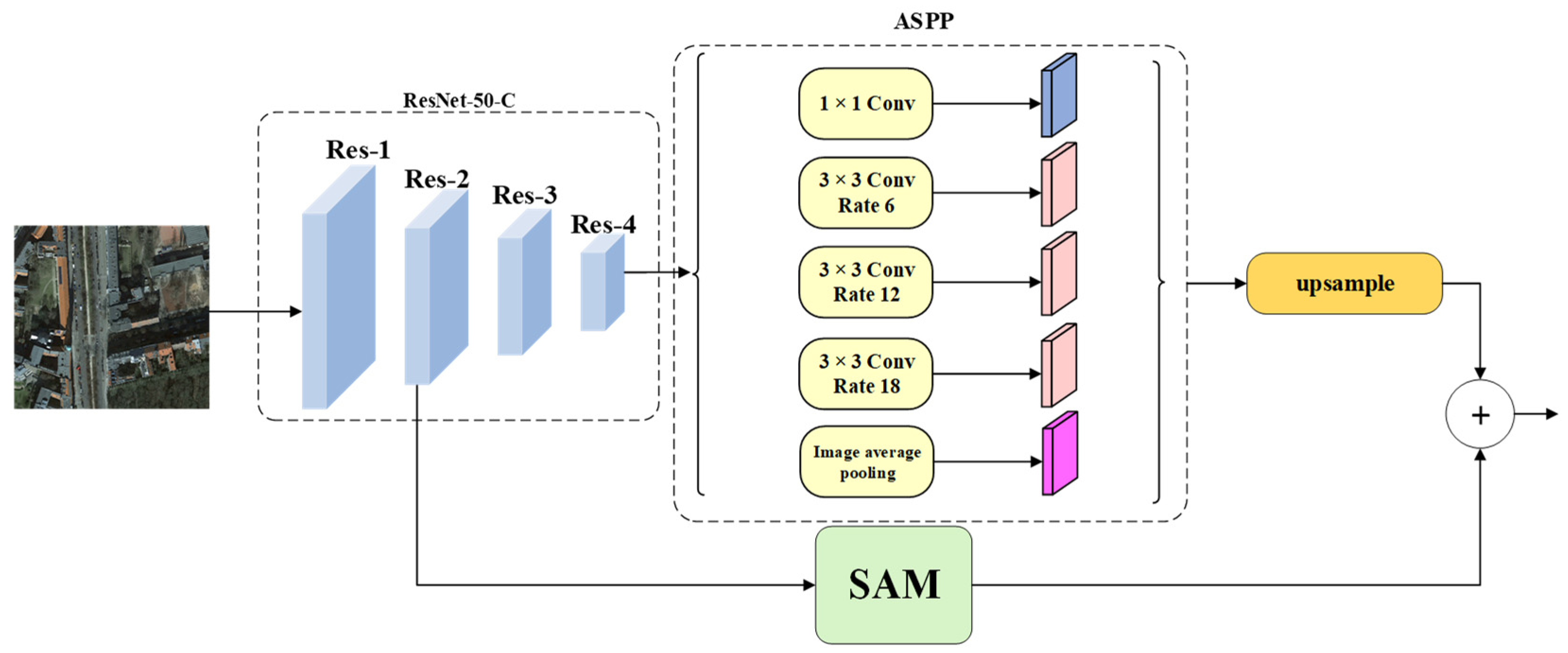
2.4. Strip Attention Net

The network structure of this paper is shown in Figure 4. The backbone part of the network uses ResNet-50-C [33] to extract the features of the input image. ResNet-50-c replaces the 7 × 7 convolution kernels in the input part of ResNet-50 [20] with three 3 × 3 convolution kernels, which significantly reduces the number of parameters and computation. Firstly, we extract the feature map of the Res-2 section in ResNet-50-C and use the SAM to extract the horizontal and vertical local feature context information of this feature map. The output of SAM is used as the low-level features $X^l$. The feature map of Res-4 in ResNet-50-C is fed into the ASPP [23] module, which obtains the global and multiscale information of the feature map by convolving the voids using different expansion rates. The output of ASPP is used as the high-level features $X^h$. Finally, the channel attention fusion module (CAF) fuses the low-level features with the elapsed high-level features and up-samples them to obtain the final prediction results.

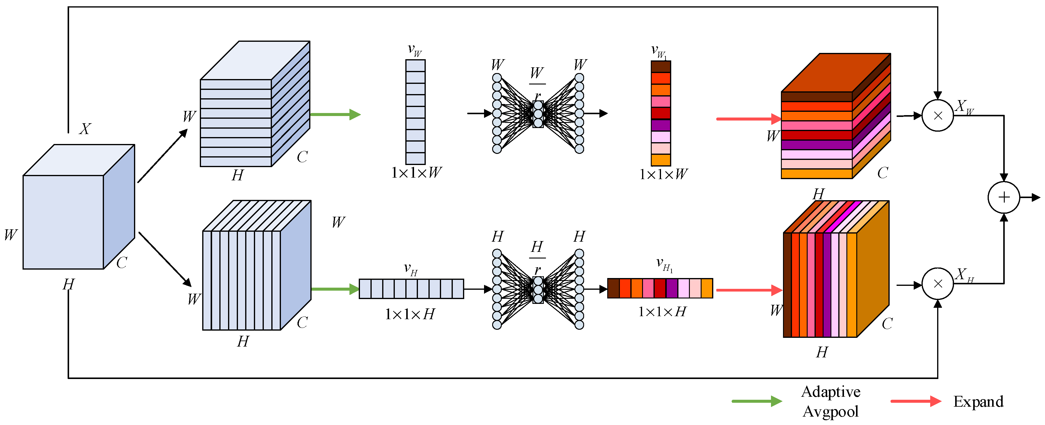
2.5. Strip Attention Module

The road span is large, narrow, and continuous. Urban roads are more regular in shape, while rural roads can be more curved. Ordinary attention modules cannot capture road features well. The network should pay more attention to the pixel distribution of rows and columns while focusing on macro-scale spatial information to be able to segment the roads better. Therefore, this paper designs a strip attention module (SAM) to focus on the pixel distribution of each row and column, which encodes finer horizontal and vertical information into local features to help the network segment roads more accurately and improve road segmentation accuracy. SAM exploits the elongated shape along the spatial direction to capture the long-range correlation of the road area to reduce the influence of the narrowband surrounding information and to capture the linear characteristics of the road.

The SAM is shown in Figure 5. Firstly, the process of column pixel feature extraction is illustrated in the upper branch of Figure 5. To study the distribution of column pixels, averaging pooling is performed for each row of $H·C$ data of the input feature mapping $X$ to determine a $W·1$-dimensional column feature vector $v_W$. Its $m^{\mathrm{th}}$ data point $v_W$is given by:

$$v_{W_m}=F_a\left(X_{W_m}\right)=\frac{1}{H·C}{\displaystyle \sum }_{i=1}^H{\displaystyle \sum }_{j=1}^C{X}_{W_m}\left(i,j\right)$$

(3)

where $F_a$denotes the adaptive average pooling and $X_{W_m}$denotes all $H·C$ data in the $m^{\mathrm{th}}$ column.

Next, the feature vector $v_W$ goes through the activation layer and the fully connected layer. This is fulfilled by first adding a fully connected layer for dimensionality reduction after the $v_W$ vector with a dimensionality reduction rate of $r$ (the value of this parameter is discussed in the first ablation study (1)), followed by a dimensionality increasing layer that returns to the $W$ dimension of the feature mapping $X$ to obtain the new feature vector $v_{W_1}$. $v_{W_1}$ as expressed by:

$$v_{w_1}=\sigma \left(W_2\delta \left(W_1{v}_W\right)\right)$$

(4)

where $\delta$ refers to the ReLU function and $\sigma$refers to the sigmoid function. $W_1\in {ℝ}^{\frac{W}{r}\times W}$, $W_2\in {ℝ}^{W\times \frac{W}{r}}$, and $W_1$ and $W_2$ are two fully connected layer operations.

The dimensional expansion of $v_{W_1}$ restores it to the size of $H·W·C$, and then multiplies it with the input feature map $X$ to obtain the new feature map $X_W$. Up to this point, we refer to the previous process as the column attention part.

Similarly, to evaluate the distribution of row pixel features, adaptive averaging pooling of $W\times C$ data per row of the input feature mapping $X$ is performed to obtain a $1·H$-dimensional column feature vector $v_H$. Its $n^{th}$data point $v_{H_n}$ is given by:

$$v_{H_n}=F_a\left(X_{H_n}\right)=\frac{1}{W·C}{\displaystyle \sum }_{i=1}^W{\displaystyle \sum }_{j=1}^C{X}_{H_n}\left(i,j\right)$$

(5)

where $F_a$denotes the adaptive average pooling and $X_{H_n}$denotes all $W·C$ data in the $n^{\mathrm{th}}$ row.

Similarly, the dimension of the feature vector $v_H$ is reduced and then increased by the fully connected layer, and the new feature vector $v_{H_1}$ is obtained thus:

$$v_{H_1}=\sigma \left(W_4\delta \left(W_3{v}_H\right)\right)$$

(6)

where $\delta$ refers to the ReLU function and $\sigma$refers to the sigmoid function. $W_3\in {ℝ}^{\frac{H}{r}\times H}$, $W_4\in {ℝ}^{H\times \frac{H}{r}}$, and $W_1$ and $W_2$ are two fully connected layer operations.

The dimensional expansion of $v_{H_1}$ restores it to the size of $H·W·C$, and then multiplies it with the input feature map $X$ to get the new feature map $X_H$. Up to this point, we refer to the previous process as the row attention part.

The feature maps $X_W$ of column attention and $X_H$ of row attention are matrix summed to acquire the final low-level feature output $X^l$, which is helpful to improve the accuracy of road extraction.

2.6. Channel Attention Fusion Module

The structure of the channel attention fusion module (CAF) is shown in Figure 6. The feature map generated in ResNet-50-C in the Res-2 stage is larger in size and has fewer channels. As it retains more spatial position information, the SAM is used to extract the spatial position information from it. The spatial position information can help the network to locate roads more accurately. The feature map after the SAM processing is used as the low-level feature $X^l$. The feature map generated in the Res-4 stage is smaller in size and has a larger number of channels. It has highly aggregated category information and is processed by atrous spatial pyramid pooling (ASPP) to obtain the high-level feature $X^h$.

The CAF module first processes the low-level feature $X^h$. Adaptive maximum pooling is performed on its channel dimension to obtain a $1·1·C$ vector $v_{max}$. Its $k$-th data $v_{max}{}^k$ is calculated as follows:

$$v_{max}{}^k=F_m\left(X^{h^k}\right)=\frac{1}{H·W}{\displaystyle \sum }_{i=1}^H{\displaystyle \sum }_{j=1}^W{X}^{h^k}\left(i,j\right)$$

(7)

where $F_m$denotes the adaptive maximum pooling and $X^{h^k}$ denotes all $H·W$ data in the $k$-th row.

The dimension of the feature vector $v_{max}$ is reduced and then increased by the fully connected layer, and the new feature vector $v_{max1}$ is obtained. Its calculation formula is as follows:

$$v_{max1}=\sigma \left(W_6\delta \left(W_5{v}_{max}\right)\right)$$

(8)

where $\delta$ refers to the ReLU function and $\sigma$refers to the sigmoid function. $W_5\in {ℝ}^{\frac{C}{16}\times C}$, $W_6\in {ℝ}^{C\times \frac{C}{16}}$, and $W_1$ and $W_2$ are two fully connected layer operations.

Adaptive average pooling is performed on its channel dimension to obtain a $1·1·C$ vector $v_{avg}$. Its $l$-th data $v_{avg}{}^l$ is calculated as follows:

$$v_{avg}{}^l=F_a\left(X^{h^l}\right)=\frac{1}{H·W}{\displaystyle \sum }_{i=1}^H{\displaystyle \sum }_{j=1}^W{X}^{h^l}\left(i,j\right)$$

(9)

where $F_a$denotes the adaptive average pooling and $X^{h^l}$ denotes all $H·W$ data in the $l$-th row.

The dimension of feature vector $v_{avg}$ is reduced and then increased by the fully connected layer, and the new feature vector $v_{avg1}$ is obtained. Its calculation formula is as follows:

$$v_{avg1}=\sigma \left(W_8\delta \left(W_7{v}_{avg}\right)\right)$$

(10)

where $\delta$ refers to the ReLU function and $\sigma$refers to the sigmoid function. $W_7\in {ℝ}^{\frac{C}{16}\times C}$, $W_8\in {ℝ}^{C\times \frac{C}{16}}$, and $W_1$ and $W_2$ are two fully connected layer operations.

For the reduction rate of the channel attention, this paper refers to the reduction rate setting of SENet [26], where the network has the highest accuracy at a reduction rate of 16.

Vector $v_{max1}$ and vector $v_{avg1}$ highly aggregate the category information of high-level features. The sum of both results is $v^h$. The final result is obtained by multiplying this vector with the low-level feature $X^l$. The low-level feature is rich in position information, and the high-level feature is rich in category information, and the two are fused by using a multiplication operation.

3. Results and Analysis

In this paper, the network shown in Figure 7 is used as the baseline network for ablation experiments. The input images are extracted features by ResNet-50-C, then further extracted features by the ASPP module, and up-sampled to obtain the results.

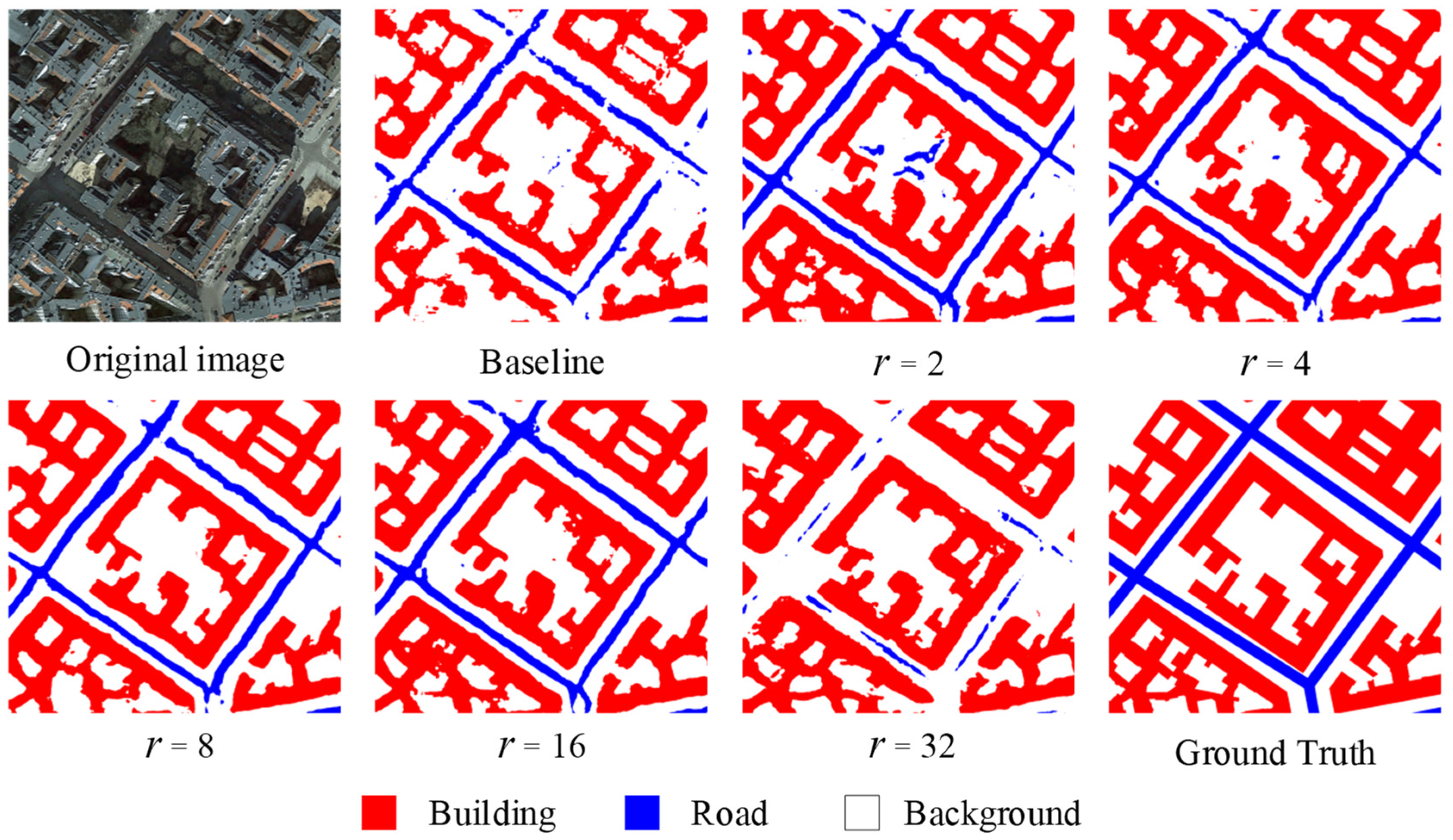
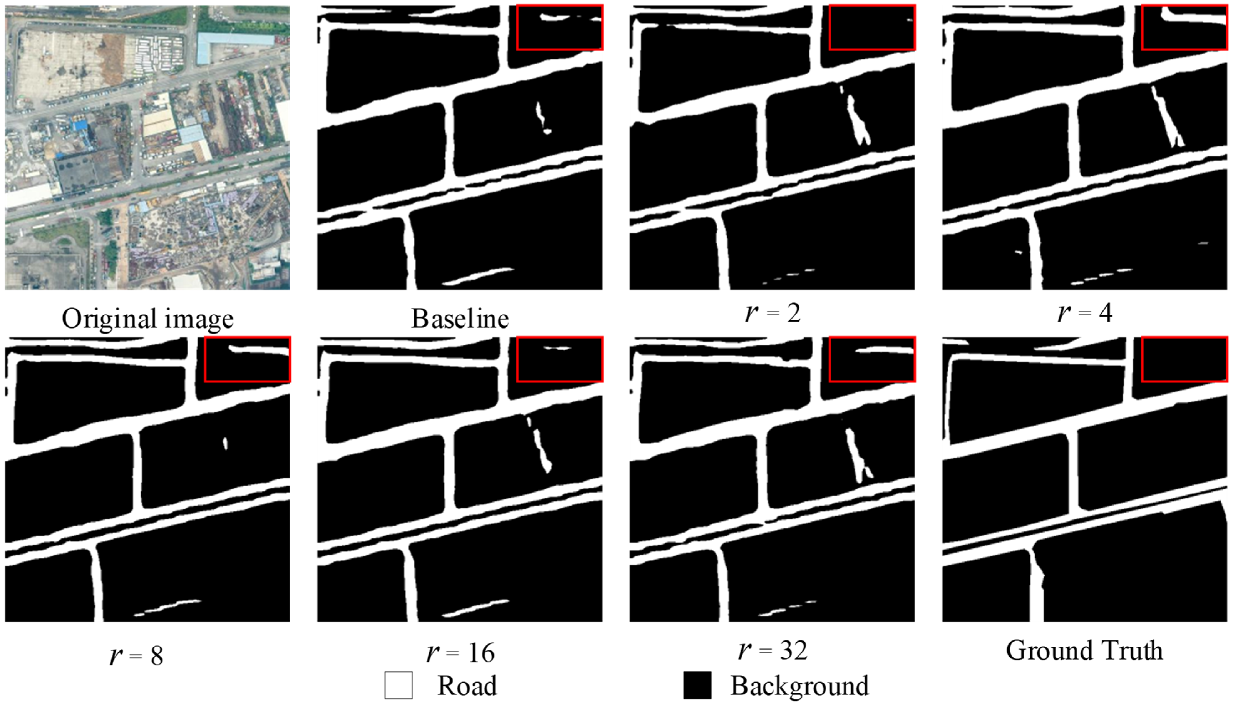
3.1. Comparison of the Reduction Rate $r$

In Section 2, it is found that setting different values of $r$ have an impact on the accuracy of the network through experiments. As shown in the Figure 8, we added SAM with different $r$ values after Res-2 and added them with high-level features to test the most appropriate value of $r$.

Considering the effect of random errors, all ablation experiments in this thesis were conducted with five replications, and the data listed in the table are the average values.

The experimental results of setting different dimensionality reduction rates $r$ based on the CITY-OSM dataset are shown in

Table 1. Comparison of dimensionality reduction rates of strip attention modules based on the CITY-OSM dataset. (Data in bold are the best results.).

Method	Per-Class IoU (%)			MIoU (%)
	Background	Building	Road
Baseline	83.44	48.61	76.3	69.45
$r=2$	83.54	52.74	76.93	71.07
$r=4$	83.62	52.06	76.97	70.88
$r=8$	83.58	52.43	77.0	71.01
$r=16$	83.65	53.31	77.07	71.34
$r=32$	82.78	46.32	76.05	68.39

.

From the data in Table 1, the MIoU values of the network with the addition of the SAM, at $r=\left\{2,4,8,16\right\}$, are higher than those of the baseline network, and the IoU values of each category are also improved.

A comparison of the visual results of the Table 1 experiments is shown in Figure 9. As can be seen from Figure 9, when $r=\left\{2,4,8,16\right\}$, the segmentation results of the network with SAM are better than those of the baseline network. When $r$ = 16, the road in the figure almost has no interruption phenomenon, which is better than the segmentation results of other dimension reduction rate networks. This is consistent with the data results in Table 1.

The results based on the DeepGlobe dataset set with different dimensionality reduction rates are shown in

Table 2. Comparison of dimensionality reduction rates of strip attention modules based on the DeepGlobe dataset. (Data in bold are the best results.).

Method	Per-Class IoU(%)		MIoU (%)
	Background	Road
Baseline	98.06	62.24	80.15
$r=2$	98.10	62.43	80.27
$r=4$	98.10	62.53	80.32
$r=8$	98.07	62.67	80.37
$r=16$	98.10	62.68	80.39
$r=32$	98.10	62.36	80.23

. As can be seen from Table 2, the MIoU value of all the networks with SAM is higher than that of the baseline network. The best result is also obtained when $r=16$.

A comparison of the visual results for the Table 2 experiments is shown in Figure 10. The area marked by the red box in the figure shows that the segmented road of the network with the addition of the SAM is clearer and can reduce the number of road disconnections. The best results are obtained when $r=16$. This is consistent with the experimental data obtained in Table 2.

The results based on the CHN6-CUG dataset set with different dimensionality reduction rates are shown in

Table 3. Comparison of dimensionality reduction rates of strip attention modules based on the CHN6-CUG dataset. (Data in bold are the best results.).

Method	Per-class IoU (%)		MIoU (%)
	Background	Road
Baseline	97.12	60.13	78.63
$r=2$	97.18	60.28	78.73
$r=4$	97.23	60.71	78.97
$r=8$	97.25	60.99	79.12
$r=16$	97.26	61.73	79.50
$r=32$	97.18	60.17	78.67

. As can be seen from Table 3, the MIoU value of all the networks with the SAM is higher than that of the baseline network. When $r=16$, the IoU value of the road is 1.6% higher than that of the baseline network, and the MIoU value is 0.87% higher than that of the baseline network. In this case, the optimal segmentation result is obtained. This indicates that the module has the best performance when $r=16$.

A comparison of the visual results for the Table 3 experiments is shown in Figure 11. The area marked by the red box in the figure shows that the false segmentation rate is the lowest when $r=16$.

It can be seen from the above three experiments that the SAM has the best performance when the dimensionality reduction rate is set to 16.

3.2. Module Validity Analysis

Again, the network shown in Figure 7 is used as the baseline network for the analysis of module effectiveness. The SAM and the CAF are added successively after the baseline network to evaluate the module effectiveness. The $r=16$ is set uniformly in the experiments, and

Table 4. Module validity analysis based on CITY-OSM dataset. (Data in bold are the best results.)

Method	Per-Class IoU (%)			MIoU (%)
	Background	Building	Road
Baseline	83.44	48.61	76.30	69.45
Baseline+SAM (Res-1)	83.42	51.28	76.51	70.40
Baseline+SAM (Res-2)	83.65	53.31	77.07	71.34
Baseline+SAM (Res-3)	83.29	50.64	76.58	70.17
Baseline+SAM+CAF (average)	83.96	50.72	77.13	70.60
Baseline+SAM+CAF (max)	83.53	52.45	77.10	71.03
Baseline+SAM+CAF (Ours)	84.26	54.78	77.55	72.20

shows the segmentation accuracy when different modules are added separately to the baseline network based on the CITY-OSM dataset.

We performed ablation experiments on the position of the SAM module addition. The SAM module was added to Res-1, Res-2, and Res-3, respectively, for the experiment. We also discussed the pooling operation in the CAF module. We tried using maximum pooling only versus average pooling only and both together and compared them.

The data in the table show that by adding the modules proposed in this paper, the IoU of all three categories is improved, which proves the effectiveness of each module. Adding the SAM to the baseline network increases the IoU value of roads by 0.77% and the IoU value of buildings by 4.70%. This indicates that the addition of SAM enables the network to pay more attention to the spatial position information of roads and locate roads more accurately. Performance is best when the SAM module is added after the Res-2 section. The CAF module performs best when maximum pooling and average pooling are used together. After adding the CAF on top of the SAM, all three categories are improved to some extent. It is proved that CAF can extract the category information of high-level features and integrate them with the other low-level features well and obtain a better segmentation effect.

The comparison results of the visual results listed in Table 4 are shown in Figure 12. The SAM module is added after the Res-2 section, and the CAF module uses the combination of maximum pooling and average pooling. As the module increases, the road segmentation effect is found to improve, the road boundary is smoother and less disconnected, and the false segmentation rate gradually decreases. This is consistent with the numerical results in Table 4.

The results of the module effectiveness analysis based on the DeepGlobe dataset are shown in

Table 5. Module validity analysis based on the DeepGlobe dataset. (Data in bold are the best results.)

Method	Per-Class IoU (%)		MIoU (%)
	Background	Road
Baseline	98.06	62.24	80.15
Baseline + SAM (Res-1)	98.11	62.45	80.28
Baseline + SAM (Res-2)	98.10	62.68	80.39
Baseline + SAM (Res-3)	98.10	62.58	80.34
Baseline + SAM + CAF (average)	98.14	62.72	80.43
Baseline + SAM + CAF (max)	98.09	62.66	80.37
Baseline + SAM + CAF (Ours)	98.15	63.05	80.60

. Again, adding the modules proposed in this paper leads to an increase in both the IoU of each category and the overall MIoU. After adding SAM, the overall MIoU improved by 0.24% compared with the baseline network. The SAM module, when added to the Res-2 section, is better than the other two. The CAF module achieves the best segmentation when it combines maximum pooling with average pooling. After adding CAF, the overall MIoU is improved by 0.45% compared with the baseline network. These data fully illustrate the effectiveness of the module added in this paper.

The visual comparison results listed in Table 5 are shown in Figure 13. The SAM module is added after the Res-2 section, and the CAF module uses the combination of maximum pooling and average pooling. As can be seen from the red boxed part of the figure, with the addition of the module, some of the roads that could not be recognized by the baseline network are recognized and the widths of the roads are getting closer to the labeled pictures, which matches the numerical results obtained in Table 5.

The results of the module effectiveness analysis based on the CHN6-CUG dataset are shown in

Table 6. Module validity analysis based on the CHN6-CUG dataset. (Data in bold are the best results.).

Method	Per-Class IoU (%)		MIoU (%)
	Background	Road
Baseline	97.12	60.13	78.63
Baseline + SAM (Res-1)	97.11	61.29	79.20
Baseline + SAM (Res-2)	97.26	61.73	79.50
Baseline + SAM (Res-3)	97.26	61.58	79.42
Baseline + SAM + CAF (average)	97.32	62.50	79.91
Baseline + SAM + CAF (max)	97.18	62.04	79.61
Baseline + SAM + CAF (Ours)	97.35	63.08	80.22

. It can be seen that by adding the module proposed in this paper, IoU values of all categories and MIoU values are improved. The segmentation effect is getting better and better. The IoU of the road increased by 1.60% with the addition of SAM after the Res-2 section. After adding the CAF that combines maximum pooling and average pooling, the IoU of the road is improved by 1.31% compared with the baseline network.

The visual comparison results listed in Table 6 are shown in Figure 14. The SAM module is added after the Res-2 section, and the CAF module uses the combination of maximum pooling and average pooling. When no modules are added, the roads in the red box area are barely recognizable. With the addition of SAM and CAF, more and more roads are identified, and the rest of the road in the picture becomes clearer. The shape of the road is also closer to ground truth, which matches the numerical results obtained in Table 6.

The above experimental results show that the SAM can extract semantic information more accurately. The CAF can effectively extract semantic features and fuse low-level features and high-level features to improve the segmentation effect.

3.3. Comparison and Analysis

In order to evaluate the performance of SANet in road extraction, DeeplabV3 [34], APCNet [35], CCNet [36], DANet, EMANet [37], and DNLNet [38] are used for comparative experiments and analysis. DeeplabV3 introduces atrous spatial pyramid pooling to extract multi-scale information; APCNet integrates multi-scale, self-adaptation, and global-guided local affinity to design the network and obtains good results. DANet models channel attention and spatial attention to extract features. EMANet designed the expectation maximization attention mechanism (EMA), which abandons the process of calculating the attention map on the whole graph. Instead, we iterated a set of compact bases through the expectation maximization (EM) algorithm and ran the attention mechanism on this set of bases, thus greatly reducing the complexity. DNLNet increases the accuracy and efficiency of road segmentation by decoupling the non-local [39] module.

The comparison results based on the CITY-OSM dataset with other segmentation networks are shown in

Table 7. Comparison with other methods based on the CITY-OSM dataset. Data in bold are the best results.

Method	Per-class IoU (%)			MIoU (%)
	Background	Building	Road
DeepLabV3 [34]	83.44	48.61	76.30	69.45
APCNet [35]	83.75	49.42	76.77	69.98
CCNet [36]	83.32	52.76	76.50	70.86
DANet [28]	81.76	47.61	73.04	67.47
EMANet [37]	83.76	53.34	77.03	71.38
DNLNet [38]	83.95	53.00	77.12	71.36
CRANet [40]	83.29	51.35	76.84	70.49
SANet (Ours)	84.26	54.78	77.55	72.20

. The MIoU of SANet reaches 72.20%, obtaining the best segmentation results compared to other networks, and the IoU of each category is higher than the others. For the road category, the IoU value of SANet reaches 77.55%, which is 0.43% higher than that of the suboptimal DNLNet, proving the superiority and effectiveness of SANet for road segmentation. The IoU values for the background and building categories were on average about 1% higher than the other networks. The experimental results show that SANet can extract the information from various categories better and the segmentation of each pixel is more accurate.

The visual comparison of the results listed in Table 7 is shown in Figure 15. The results in the figure show that SANet has better road segmentation than other networks, the best road connectivity, the lowest number of unidentified roads, and the highest road clarity, which matches the results of the data obtained in Table 7.

The comparison results based on the DeepGlobe dataset with other segmentation networks are illustrated in

Table 8. Comparison with other methods based on the DeepGlobe dataset. Data in bold are the best results.

Method	Per-Class IoU (%)		MIoU (%)
	Background	Road
DeepLabV3 [34]	98.06	62.24	80.15
APCNet [35]	98.03	59.78	78.91
CCNet [36]	98.09	61.77	79.93
DANet [28]	97.98	61.77	79.88
EMANet [37]	98.06	61.45	79.76
DNLNet [38]	98.10	62.19	80.15
CRANet [40]	98.05	62.04	80.04
SANet (Ours)	98.15	63.05	80.60

. SANet has an IoU value of 63.05% and a MIoU value of 80.60% in the road category, both of which are improved compared with other networks, and the MIoU in the background category is also improved. From the above results, it can be seen that SAM for road design in SANet can better identify and segment roads, and CAF can better extract channel information and integrate low-level and high-level features to improve segmentation accuracy.

The visual comparison results listed in Table 8 are shown in Figure 16. SANet can segment roads that other networks failed to segment and did not mis-segment the background category as roads, proving that the network has excellent road segmentation ability, which is consistent with the data listed in Table 8.

The comparison results based on the CHN6-CUG dataset with other segmentation networks are illustrated in

Table 9. Comparison with other methods based on the CHN6-CUG dataset. Data in bold are the best results.

Method	Per-Class IoU (%)		MIoU (%)
	Background	Road
DeepLabV3 [34]	97.12	60.13	78.63
APCNet [35]	97.24	61.90	79.57
CCNet [36]	97.26	61.58	79.42
DANet [28]	97.23	60.44	78.83
EMANet [37]	97.18	62.04	79.61
DNLNet [38]	97.32	62.50	79.91
CRANet [40]	97.32	62.88	80.10
SANet (Ours)	97.35	63.08	80.22

. As can be seen from the data in the table, SANet achieves the best segmentation effect. The IoU value of the road reached 63.08%, which was the highest and 0.58% higher than the suboptimal DNLNet. SANet also has the highest MIoU value of 80.22%, which is better than other networks.

The visual comparison results listed in Table 9 are shown in Figure 17. The road in the segmentation results of SANet is complete and clear. The false segmentation rate is the lowest and is closest to the ground truth. This indicates that SANet has the best segmentation effect, which is consistent with the data listed in Table 9.

The above experimental results show that SANet has a high degree of integrity in road extraction and can segment roads that cannot be segmented by other networks, with a low false segmentation rate and good road segmentation performance.

4. Discussion

In the experimental part, we found that the SAM module can extract the position information of the road more completely. It uses long-range pooling operations and fully connected layers to make the network better at extracting long and narrow shapes. While extracting the category information in the channel of the picture, CAF fuses the position information of the low-level features with the category information of the high-level features, so that the segmentation accuracy is further improved. These results show that the accuracy of road segmentation is closely related to both category information and position information. Sufficient extraction of category information will reduce mis-segmentation. The accurate position information extracted will reduce the position error.

5. Conclusions

In this paper, a new image segmentation network (SANet) is proposed for segmenting roads from remote sensing images to solve the problem concerning the poor continuity of semantic segmentation networks in segmenting roads. The experiments show that the SAM designed in this paper can accurately extract the context information of the road and locate the road, so as to improve the accuracy of road extraction. At the same time, the experimental data also show that the proposed CAF can effectively extract the category information of the road in the feature map and fuse the low-level and high-level features. CAF can reduce the false segmentation rate and improve the segmentation accuracy.

The research results in this article show that both the position information in the low-level features and the category information in the high-level features have an impact on the segmentation effect. These two are indispensable, and we will conduct more in-depth research on their extraction methods and fusion methods in the future.

References

1. Zhou, M.; Sui, H.; Chen, S.; Wang, J.; Chen, X. BT-RoadNet: A boundary and topologically-aware neural network for road extraction from high-resolution remote sensing imagery. ISPRS J. Photogramm. Remote Sens. 2020, 168, 288–306. [Google Scholar] [CrossRef]
2. Das, S.; Mirnalinee, T.T.; Varghese, K. Use of salient features for the design of a multistage framework to extract roads from high-resolution multispectral satellite images. IEEE Trans. Geosci. Remote Sens. 2011, 49, 3906–3931. [Google Scholar] [CrossRef]
3. Lv, X.; Ming, D.; Chen, Y.Y.; Wang, M. Very high resolution remote sensing image classification with SEEDS-CNN and scale effect analysis for superpixel CNN classification. Int. J. Remote Sens. 2019, 40, 506–531. [Google Scholar] [CrossRef]
4. Lv, X.; Ming, D.; Lu, T.; Zhou, K.; Wang, M.; Bao, H. A new method for region-based majority voting CNNs for very high resolution image classification. Remote Sens. 2018, 10, 1946. [Google Scholar] [CrossRef]
5. Sardar, A.; Mehrshad, N.; Mohammad, R.S. Efficient image segmentation method based on an adaptive selection of Gabor filters. IET Image Process. 2020, 14, 4198–4209. [Google Scholar] [CrossRef]
6. Xu, D.; Zhao, Y.; Jiang, Y.; Zhang, C.; Sun, B.; He, X. Using Improved Edge Detection Method to Detect Mining-Induced Ground Fissures Identified by Unmanned Aerial Vehicle Remote Sensing. Remote Sens. 2021, 13, 3652. [Google Scholar] [CrossRef]
7. Omati, M.; Sahebi, M.R. Change detection of polarimetric SAR images based on the integration of improved watershed and MRF segmentation approaches. IEEE J. Sel. Topics Appl. Earth Observ. Remote Sens. 2018, 11, 4170–4179. [Google Scholar] [CrossRef]
8. Song, M.J.; Civco, D. Road Extraction Using SVM and Image Segmentation. Photogramm. Eng. Remote Sens. 2004, 70, 1365–1371. [Google Scholar] [CrossRef]
9. Jeong, M.; Nam, J.; Ko, B.C. Lightweight Multilayer Random Forests for Monitoring Driver Emotional Status. IEEE Access. 2020, 8, 60344–60354. [Google Scholar] [CrossRef]
10. Kass, M.; Witkin, A.; Terzopoulos, D. Snakes: Active contour models. Int. J. Comput. Vis. 1988, 1, 321–331. [Google Scholar] [CrossRef]
11. Shi, W.; Miao, Z.; Wang, Q.; Zhang, H. Spectral-spatial classification and shape features for urban road centerline extraction. IEEE Geosci. Remote Sens. Lett. 2014, 11, 788–792. [Google Scholar]
12. Ghaziani, M.; Mohamadi, Y.; Koku, A.B. Extraction of unstructured roads from satellite images using binary image segmentation. In Proceedings of the 2013 21st Signal Processing and Communications Applications Conference, Haspolat, Turkey, 24–26 April 2013; pp. 1–4. [Google Scholar]
13. Sirmacek, B.; Unsalan, C. Road network extraction using edge detection and spatial voting. In Proceedings of the 2010 20th International Conference on Pattern Recognition, Istanbul, Turkey, 23–26 August 2010; pp. 3113–3116. [Google Scholar]
14. Zhang, C.; Tang, Z.; Zhang, M.; Wang, B.; Hou, L. Developing a More Reliable Aerial Photography-Based Method for Acquiring Freeway Traffic Data. Remote Sens. 2022, 14, 2202. [Google Scholar] [CrossRef]
15. Zhang, S.; Li, C.; Qiu, S.; Gao, C.; Zhang, F.; Du, Z.; Liu, R. EMMCNN: An ETPS-Based Multi-Scale and Multi-Feature Method Using CNN for High Spatial Resolution Image Land-Cover Classification. Remote Sens. 2020, 12, 66. [Google Scholar] [CrossRef]
16. Krizhevsky, A.; Sutskever, I.; Hinton, G.E. Imagenet classification with deep convolutional neural networks. Adv. Neural Inf. Process. Syst. 2012, 60, 84–90. [Google Scholar] [CrossRef]
17. Shao, S.; Xiao, L.; Lin, L.; Ren, C.; Tian, J. Road Extraction Convolutional Neural Network with Embedded Attention Mechanism for Remote Sensing Imagery. Remote Sens. 2022, 14, 2061. [Google Scholar] [CrossRef]
18. Long, J.; Shelhamer, E.; Darrell, T. Fully convolutional networks for semantic segmentation. In Proceedings of the IEEE Conference on Computer Vision and Pattern Recognition, Boston, MA, USA, 7–12 June 2015; pp. 3431–3440. [Google Scholar]
19. Ronneberger, O.; Fischer, P.; Brox, T. U-net: Convolutional networks for biomedical image segmentation. In Proceedings of the International Conference on Medical Image Computing and Computer-Assisted Intervention, Munich, Germany, 5–9 October 2015; Springer: Cham, Switzerland, 2015; pp. 234–241. [Google Scholar]
20. He, K.; Zhang, X.; Ren, S.; Sun, J. Deep residual learning for image recognition. In Proceedings of the IEEE Conference on Computer Vision and Pattern Recognition, Las Vegas, NV, USA, 26 June–1 July 2016; pp. 770–778. [Google Scholar]
21. Zhang, Z.X.; Liu, Q.J.; Wang, Y.H. Road Extraction by Deep Residual U-Net. IEEE Geosci. Remote Sens. Lett. 2018, 15, 749–753. [Google Scholar] [CrossRef]
22. Zhao, H.; Shi, J.; Qi, X.; Wang, X.; Jia, J. Pyramid scene parsing network. In Proceedings of the IEEE Conference on Computer Vision and Pattern Recognition, Honolulu, HI, USA, 21–26 July 2017; pp. 2881–2890. [Google Scholar]
23. Chen, L.C.; Zhu, Y.; Papandreou, G.; Schroff, F.; Adam, H. Encoder-decoder with atrous separable convolution for semantic image segmentation. In Proceedings of the European Conference on Computer Vision (ECCV), Munich, Germany, 8–14 September 2018; pp. 801–818. [Google Scholar]
24. Zhou, L.; Zhang, C.; Wu, M. D-linknet: Linknet with pretrained encoder and dilated convolution for high resolution satellite imagery road extraction. In Proceedings of the IEEE Conference on Computer Vision and Pattern Recognition Workshops, Salt Lake City, UT, USA, 18–22 June 2018; pp. 182–186. [Google Scholar]
25. Chaurasia, A.; Culurciello, E. Linknet: Exploiting encoder representations for efficient semantic segmentation. In Proceedings of the IEEE Visual Communications and Image Processing, St. Petersburg, FL, USA, 10–13 December 2017; pp. 1–4. [Google Scholar]
26. Hu, J.; Shen, L.; Sun, G. Squeeze-and-Excitation Networks. In Proceedings of the 2018 IEEE/CVF Conference on Computer Vision and Pattern Recognition, Salt Lake City, UT, USA, 18–23 June 2018; pp. 7132–7141. [Google Scholar]
27. Woo, S.; Park, J.; Lee, J.Y.; Kweon, I.S. Cbam: Convolutional block attention module. In Proceedings of the European Conference on Computer Vision (ECCV), Munich, Germany, 8–14 September 2018; pp. 3–19. [Google Scholar]
28. Fu, J.; Liu, J.; Tian, H.; Li, Y.; Bao, Y.; Fang, Z.; Lu, H. Dual Attention Network for Scene Segmentation. In Proceedings of the 2019 IEEE/CVF Conference on Computer Vision and Pattern Recognition (CVPR), Long Beach, CA, USA, 15–20 June 2019; pp. 3146–3154. [Google Scholar]
29. Yu, C.; Wang, J.; Gao, C.; Yu, G.; Shen, C.; Sang, N. Context prior for scene segmentation. In Proceedings of the IEEE/CVF conference on computer vision and pattern recognition, Seattle, WA, USA, 14–19 June 2020; pp. 12416–12425. [Google Scholar]
30. Kaiser, P.; Wegner, J.D.; Lucchi, A.; Jaggi, M.; Hofmann, T.; Schindler, K. Learning aerial image segmentation from online maps. IEEE Trans. Geosci. Remote Sens. 2017, 55, 6054–6068. [Google Scholar] [CrossRef]
31. Zhu, Q.; Zhang, Y.; Wang, L.; Zhong, Y.; Guan, Q.; Lu, X.; Zhang, L.; Li, D. A Global Context-aware and Batch-independent Network for road extraction from VHR satellite imagery. ISPRS J. Photogramm. Remote Sens. 2021, 175, 353–365. [Google Scholar] [CrossRef]
32. MMSegmentation Contributors. MMSegmentation: Openmmlab Semantic Segmentation Toolbox and Benchmark. 2020. Available online: https://github.com/open-mmlab/mmsegmentation (accessed on 11 August 2020).
33. He, T.; Zhang, Z.; Zhang, H.; Zhang, Z.; Xie, J.; Li, M. Bag of Tricks for Image Classification with Convolutional Neural Networks. In Proceedings of the IEEE/CVF Conference on Computer Vision and Pattern Recognition (CVPR), Long Beach, CA, USA, 15–20 June 2019; pp. 558–567. [Google Scholar]
34. Chen, L.C.; Papandreou, G.; Schroff, F.; Adam, H. Rethinking atrous convolution for semantic image segmentation. arXiv 2017, arXiv:1706.05587. [Google Scholar]
35. He, J.; Deng, Z.; Zhou, L.; Wang, Y.; Qiao, Y. Adaptive Pyramid Context Network for Semantic Segmentation. In Proceedings of the IEEE/CVF Conference on Computer Vision and Pattern Recognition (CVPR), Long Beach, CA, USA, 15–20 June 2019; pp. 7511–7520. [Google Scholar]
36. Huang, Z.; Wang, X.; Wei, Y.; Huang, L.; Huang, T.S. CCNet: Criss-Cross Attention for Semantic Segmentation. In Proceedings of the 2019 IEEE/CVF International Conference on Computer Vision (ICCV), Seoul, Korea, 27 October–2 November 2019; pp. 603–612. [Google Scholar]
37. Li, X.; Zhong, Z.; Wu, J.; Yang, Y.; Lin, Z.; Liu, H. Expectation-Maximization Attention Networks for Semantic Segmentation. In Proceedings of the IEEE/CVF International Conference on Computer Vision (ICCV), Seoul, Korea, 27 October–2 November 2019; pp. 9167–9176. [Google Scholar]
38. Yin, M.; Yao, Z.; Cao, Y.; Li, X.; Zhang, Z.; Lin, S.; Hu, H. Disentangled non-Local neural networks. In Proceedings of the European Conference on Computer Vision (ECCV), Glasgow, KY, USA, 23–28 August 2020; pp. 191–207. [Google Scholar]
39. Wang, X.; Girshick, R.; Gupta, A.; He, K. Non-local Neural Networks. In Proceedings of the 2018 IEEE/CVF Conference on Computer Vision and Pattern Recognition (CVPR), Lake Tahoe, NV, USA, 12–15 March 2018; pp. 7794–7803. [Google Scholar]
40. Li, S.; Liao, C.; Ding, Y.; Hu, H.; Jia, Y.; Chen, M.; Xu, B.; Ge, X.; Liu, T.; Wu, D. Cascaded Residual Attention Enhanced Road Extraction from Remote Sensing Images. ISPRS Int. J. Geo.-Inf. 2022, 11, 9. [Google Scholar] [CrossRef]
Figure 1. Test set images of dataset I: (a)true-color, (b)ground-truth maps.
Remotesensing 14 04516 g001
Figure 2. Test set images of dataset II: (a) true-color, (b) ground-truth maps.
Remotesensing 14 04516 g002
Figure 3. Test set images of dataset III: (a) true-color, (b) ground-truth maps.
Remotesensing 14 04516 g003
Figure 4. Structure of our proposed SANet.
Remotesensing 14 04516 g004
Figure 5. Strip Attention Module.
Remotesensing 14 04516 g005
Figure 6. Channel Attention Fusion Module.
Remotesensing 14 04516 g006
Figure 7. Structure of Baseline.
Remotesensing 14 04516 g007
Figure 8. Structure of ablation study for the value of r comparison.
Remotesensing 14 04516 g008
Figure 9. Comparison of visual results of dimensionality reduction based on the CITY-OSM dataset.
Remotesensing 14 04516 g009
Figure 10. Comparison of visual results of dimensionality reduction based on the DeepGlobe dataset.
Remotesensing 14 04516 g010
Figure 11. Comparison of visual results of dimensionality reduction based on the CHN6-CUG dataset.
Remotesensing 14 04516 g011
Figure 12. Comparison of visual results of module validity analysis based on CITY-OSM dataset.
Remotesensing 14 04516 g012
Figure 13. Comparison of visual results of module validity analysis based on DeepGlobe dataset.
Remotesensing 14 04516 g013
Figure 14. Comparison of visual results of module validity analysis based on CHN6-CUG dataset.
Remotesensing 14 04516 g014
Figure 15. Comparison of visual results of each method based on CITY-OSM dataset.
Remotesensing 14 04516 g015
Figure 16. Comparison of visual results of each method based on DeepGlobe dataset.
Remotesensing 14 04516 g016
Figure 17. Comparison of visual results of each method based on the CHN6-CUG dataset.
Remotesensing 14 04516 g017