Article

Segmentation and Connectivity Reconstruction of Urban Rivers from Sentinel-2 Multi-Spectral Imagery by the WaterSCNet Deep Learning Model

1
Shanghai Carbon Data Research Center, Key Laboratory of Low-Carbon Conversion Science and Engineering, Shanghai Advanced Research Institute, Chinese Academy of Sciences, Shanghai 201210, China
2
University of Chinese Academy of Sciences, Beijing 100049, China
*
Author to whom correspondence should be addressed.
Remote Sens. 2023, 15(19), 4875; https://doi.org/10.3390/rs15194875
Submission received: 26 July 2023 / Revised: 28 September 2023 / Accepted: 6 October 2023 / Published: 8 October 2023

Abstract

:
Quick and automatic detection of the distribution and connectivity of urban rivers and their changes from satellite imagery is of great importance for urban flood control, river management, and ecological conservation. By improving the E-UNet model, this study proposed a cascaded river segmentation and connectivity reconstruction deep learning network model (WaterSCNet) to segment urban rivers from Sentinel-2 multi-spectral imagery and simultaneously reconstruct their connectivity obscured by road and bridge crossings from the segmentation results. The experimental results indicated that the WaterSCNet model could achieve better river segmentation and connectivity reconstruction results compared to the E-UNet, U-Net, SegNet, and HRNet models. Compared with the classic U-Net model, the MCC, F1, Kappa, and Recall evaluation metrics of the river segmentation results of the WaterSCNet model were improved by 3.24%, 3.10%, 3.36%, and 3.93%, respectively, and the evaluation metrics of the connectivity reconstruction results were improved by 4.25%, 4.11%, 4.37%, and 4.83%, respectively. The variance of the evaluation metrics of the five independent experiments indicated that the WaterSCNet model also had the best robustness compared to the other four models.

Graphical Abstract

1. Introduction

With the process of global urbanization, especially in developing countries experiencing rapid economic growth, continuous urban expansion and redevelopment have caused constant changes in the distribution of small and medium-sized urban rivers. Urban rivers serve as transportation routes for water and various nutrients, as water storage and flood drainage facilities, and as important regulators of local micro-climates and supports of local biodiversity. Therefore, the use of remote sensing technology to quickly and automatically detect the distribution and connectivity of urban rivers and their changes is of great importance for urban flood control, river management, ecological protection, and urban functional planning.
In natural environments, rivers flow downstream under the force of gravity. Therefore, some widely used pixel-based flow detection algorithms, such as D8 [1] and D-infinity [2], use digital elevation data to extract the distribution and connectivity of rivers. Recently, a number of methods [3,4] have also been developed to integrate Sentinel-2 multi-spectral imagery [5] with digital elevation data to extract river distribution and connectivity. However, in complex urban environments, tall buildings and artificial lowlands can make it very difficult to extract rivers based on digital elevation data [3], and high spatial resolution urban digital elevation data are also very expensive [6].
High spatial resolution satellite remote sensing imagery can also be used for river detection. Traditional methods use morphology [7], threshold [8], the water body index [9,10,11], and texture features [12] for river detection from satellite imagery. Most of these traditional methods require manual specification of thresholds, adjustment of parameters, use of manually determined features, or manual post-processing, which leads to high uncertainty in the river detection results [12,13].
With the development of deep learning, various end-to-end structures based on a convolutional neural network (CNN) [14] have emerged, such as U-Net [15], U-Net++ [16], E-UNet [17], SegNet [18], and HRNet [19], which can automatically extract high-level information from satellite imagery without a tedious manual feature extraction process [20]. U-Net [15] is a U-shaped encoder–decoder segmentation network with skip connections. The encoder–decoder structure extracts general features, and the skip connections reintroduce detailed features back into the decoder. U-Net utilizes both general and detailed features to achieve high segmentation accuracy [21,22]. U-Net++ [16] has a nested U-Net architecture with dense convolution blocks on skip connections and a deep supervision design nested at the top level of the network. The dense convolution blocks can bridge the semantic gap between encoder and decoder feature maps, and the deep supervision design can improve segmentation performance through model pruning [16,23]. E-UNet [17] enhances UNet’s encoder–decoder structure by adding a multi-spectral three-dimensional convolution (MSD) path module [24] to capture nonlinear relationships between multi-spectral bands of adjacent pixels [25,26,27], and a multi-scale pooling (MSP) block [28] to perceive texture relationships and information at multiple spatial scales. Three-dimensional convolution is mainly used in the segmentation of hyper-spectral data [26,27], and is also widely used in multi-spectral and hyper-spectral image fusion [25] and multi-spectral time series image processing [24]. These two enhancements allow E-UNet to segment objects with large scale differences from multi-spectral remote sensing imagery [17]. SegNet [18] is a CNN for semantic image segmentation. It consists of an encoder network and a corresponding decoder network followed by a pixel-wise classification layer. HRNet [19] is a general purpose CNN for tasks such as semantic segmentation, object detection, and image classification. It starts with a high-resolution convolution stream, gradually adds high-to-low resolution convolution streams one by one, and connects the multi-resolution streams in parallel [19]. Therefore, HRNet is able to maintain high resolution representations throughout the process.
Miao et al. [29] proposed a restricted receptive field deconvolution network, which solved the problem of weak pixel neighborhood correlation, to segment water bodies from Google Earth images. Chen et al. [30] proposed combining the CNN with a superpixel method for water body segmentation in complex urban backgrounds from GaoFen-2 satellite imagery [31].
Although relatively good river detection results can be obtained using high spatial resolution satellite imagery, which typically contains only the red, green, blue, and near-infrared spectral bands, the segmentation accuracy is significantly reduced when the river is shadowed by surrounding buildings or when the river color changes due to spatial and temporal variations [32]. Therefore, multi-spectral satellite imagery, which can provide more spectral information, is increasingly being used for river detection and other object recognition tasks [33,34,35].
Additional spectral information in multi-spectral satellite imagery can also improve the river detection performance of deep learning methods [36]. Isikdogan et al. [37] proposed a full CNN called Deep-WaterMap that could effectively segment surface water from Landsat-7 [38] while reducing the probability of false detection of snow, ice, and cloud shadows as water surfaces. Jing et al. [39] used a multi-layer perceptron [40] to extract water bodies from Landsat-8 imagery [41] and achieved superior performance compared to the water body index and maximum likelihood estimation methods. Xia et al. [42] introduced a separable attention residual network that utilized attention modules of different scales to combine deep and shallow feature information for river segmentation. Furthermore, Fan et al. [13] proposed a river segmentation model based on a composite attention network to accurately detect complex details such as river boundaries and portions of rivers obscured by road and bridge crossings from Landsat-8 satellite imagery [41].
Due to road and bridge crossings, urban rivers supposed to be continuous are usually detected from satellite imagery as discontinuous segments. To reconstruct the connectivity of disconnected urban rivers extracted from satellite imagery, Zhang et al. [34] proposed a method that gradually removed river discontinuities by iteratively splitting water bodies and connecting broken river segments. However, Zhang’s method had a tendency to erroneously connect two different rivers that are close to each other. Edge link algorithms [43,44], which are commonly used to close fracture curves, can also be used to connect adjacent river segments separated by small fractures, but they are unsuitable for reconstructing connectivity of small and medium-sized rivers with large portions obscured by bridge and road crossings.
The connectivity of urban rivers is of great importance in understanding the ecological and environmental interactions and impacts between them. In order to reduce tedious manual work and automate the processing of river segmentation and connectivity reconstruction from satellite remote sensing imagery, in this study, a cascaded river segmentation and connectivity reconstruction deep learning network model (WaterSCNet) was proposed to segment urban rivers and reconstruct their connectivity from Sentinel-2 multi-spectral imagery [5]. The WaterSCNet model was improved from the E-UNet model [17] by adding a soft attention gate mechanism [45] to the encoder–decoder structure. The soft attention gate mechanism, which includes channel attention [46], spatial attention [47], or a combination of both [48], can be trained by gradient backpropagation [49] and has been extensively studied and implemented in intelligent image recognition tasks [50,51]. The attention gates in the WaterSCNet model merge spatial features from the encoder with spectral features from the MSD path module, allowing the model to adaptively focus on specific regions of input images as in Schlemper’s study [49]. Thus, the attention gates can help the WaterSCNet model improve its performance.
There are two innovations in this study: first, integrating the MSD path module, the MSP block, and the soft attention gate mechanism into the U-Net encoder–decoder structure improves the segmentation performance for rivers, especially small rivers in complex urban environments, from multi-spectral imagery; second, by cascading two deep learning networks, the river segmentation and connectivity reconstruction processes are automated, reducing the tedious manual work typically required for river connectivity reconstruction tasks.
The rest of the paper is organized as follows: Section 2 details the proposed WaterSCNet model, Section 3 describes the experimental data, model training, experimental design, and evaluation metrics, Section 4 presents the experimental results and discussion, and finally, conclusions are given in Section 5.

2. Methods

2.1. The WaterSCNet Model

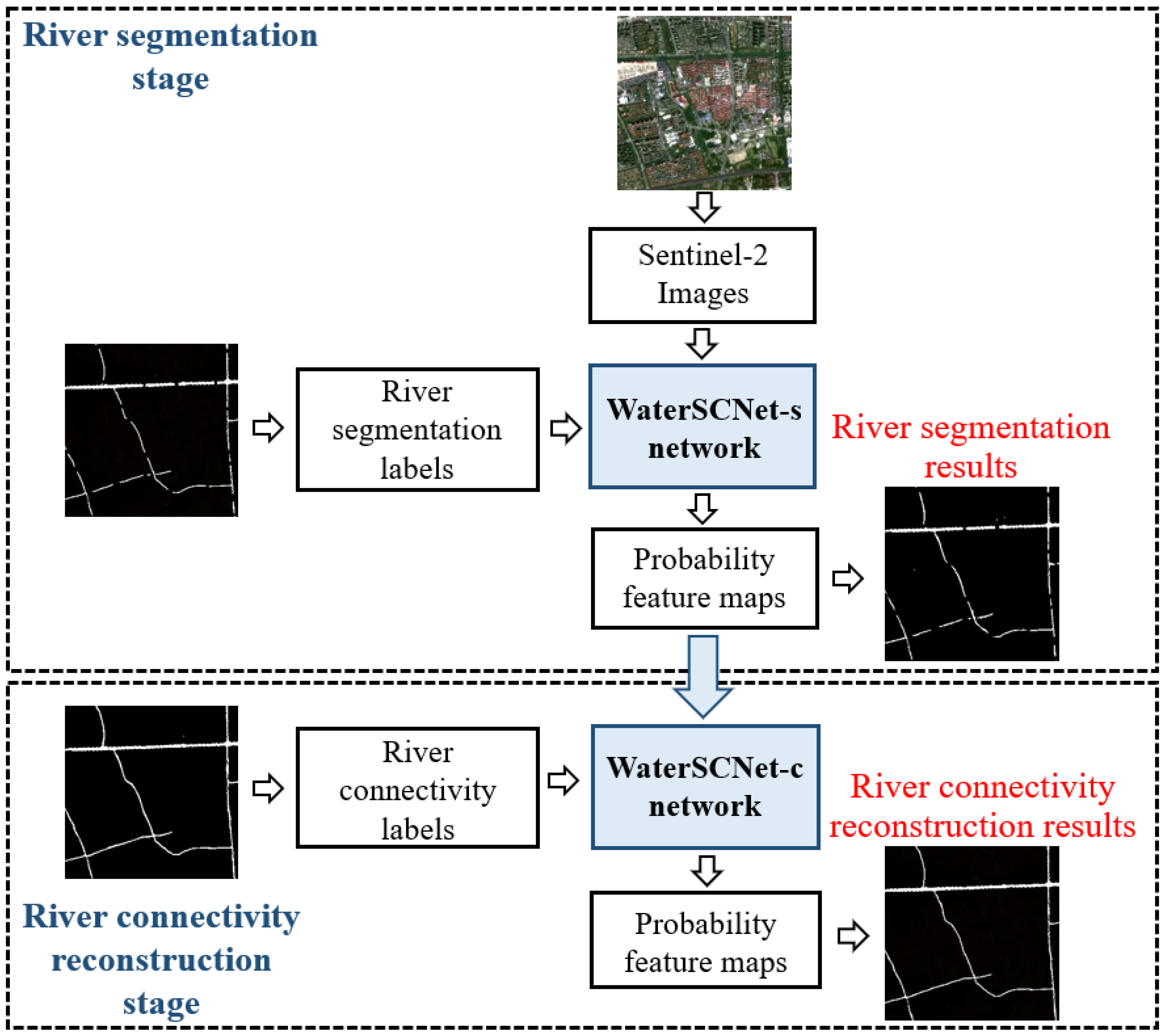
As shown in Figure 1, the proposed WaterSCNet model is an end-to-end deep learning network consisting of two cascaded subnetworks, named WaterSCNet-segmentation (WaterSCNet-s) and WaterSCNet-connection (WaterSCNet-c), respectively, to achieve segmentation and connectivity reconstruction of urban rivers.

2.2. River Segmentation Subnetwork: WaterSCNet-s

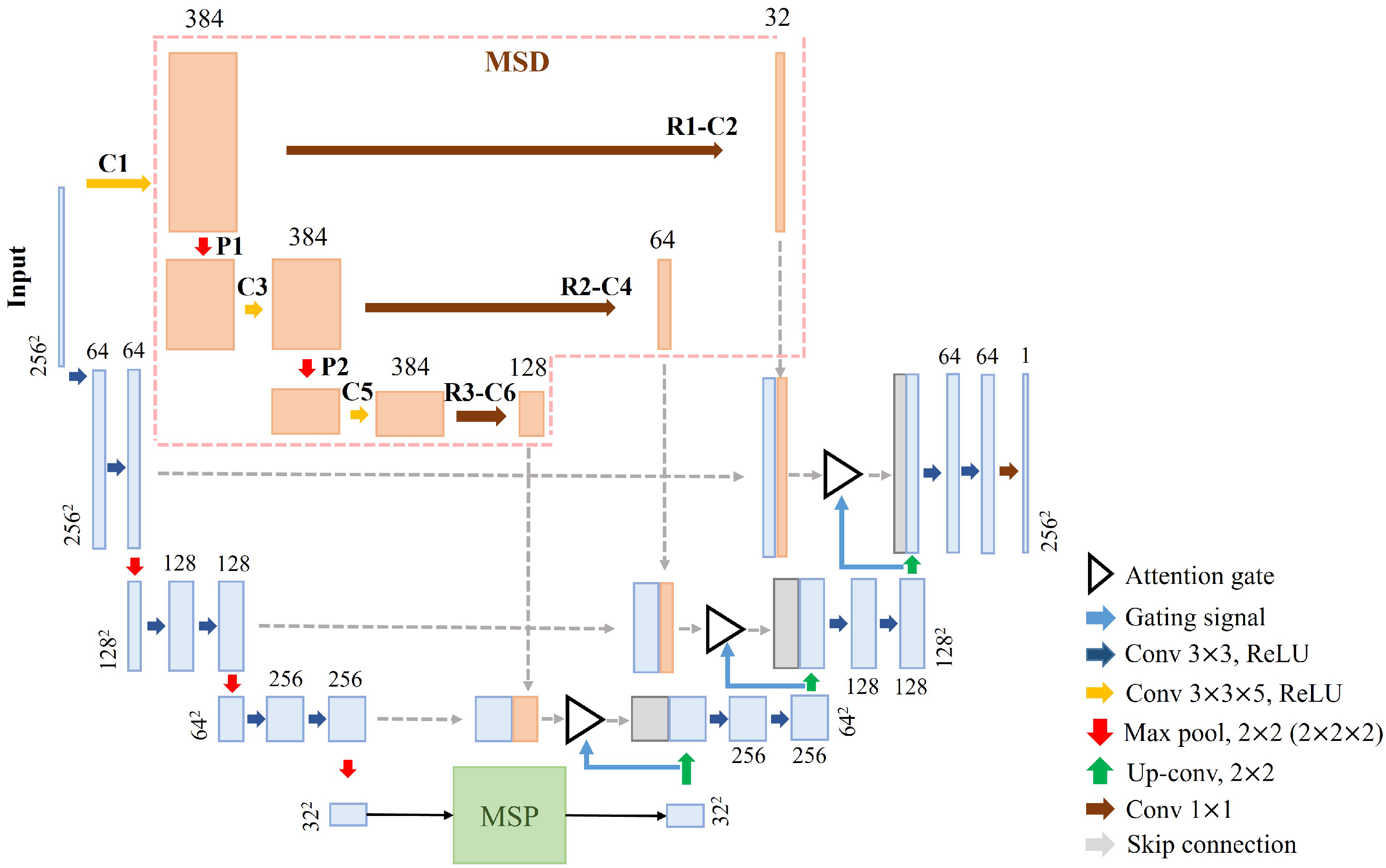
As shown in Figure 2, the WaterSCNet-s was improved from the Enhanced U-Net (E-UNet) architecture [17], which is capable of semantic segmentation of multi-spectral remote sensing imagery, for the task of urban river segmentation.
The WaterSCNet-s consists of three parts, a U-shaped symmetric encoder and decoder structure, a multi-spectral three-dimensional convolution (MSD) path module and a multi-scale pooling (MSP) block.

2.2.1. The U-Shaped Encoder and Decoder Structure

A U-shaped encoder and decoder structure, similar to the classic U-Net model [15], is the backbone of the WaterSCNet-s subnetwork. The U-shaped encoder and decoder has four layers. Each layer in the encoder performs two convolution and down-sampling operations to extract features from the input multi-spectral image, and each layer in the decoder performs up-sampling and convolution operations to progressively restore the image resolution. The dimensionality of the encoder input data is N × N × M , where N is the number of pixels in two-dimensional space and M is the number of spectral bands. The skip connection between the encoder and the decoder at each layer fuses low-level morphological features with high-level semantic features to preserve critical spatial information that might otherwise be lost during the multiple down-sampling operations.
As shown in Figure 2, in order to reduce false-positive segmentations for small rivers with large shape variations, following the work of Schlemper [49] and Oktay [45], an additive attention gate (AAG) was added in front of the decoder in each of the top three layers to automatically localize the object of interest and help the model improve its overall segmentation performance.
The input to the AAG is a concatenation of the spatial feature map extracted by the encoder and the corresponding spectral feature map extracted by the MSD path module. The concatenated feature maps are semantically discriminative at each encoding layer. The coarse spatial feature map captures contextual information and highlights the category and location of foreground objects. The gating signal up-sampled from the coarse spatial feature map can gate the AAG to disambiguate irrelevant and noisy responses in the input feature map. Therefore, the AGGs in the model can progressively suppress feature responses in irrelevant background regions and guide the model to focus on the object of interest in the foreground content of the image.
Figure 3 shows how the AGG works. First, the input and the gating signal of the AGG are linearly transformed into the same vector space by W i and W g , respectively. Then, the two linearly transformed results are summed by the additive attention method [52,53].
The summation result is first processed by an element-wise rectified linear unit (ReLU) function [54] and then transformed back to the input feature space by a linear transformation of W s . After a sigmoid activation function [55] is applied to restrict the range of attention weight Φ to [0,1], the attention weight Φ is multiplied by the input to obtain the attention feature map, as in Jian’s study [56].
The three linear transformations in the AGG are computed using channel-wise 1 × 1 two-dimensional convolutions as in Schlemper’s study [49]. The W i , W g , and W s of these linear transformations can be trained using standard back-propagation approaches [49,57]. Thus, the WaterSCNet model can be trained from scratch in a standard way similar to the training of fully convolutional network models.

2.2.2. The MSD Path Module

Following Dui’s work of E-UNet [17], an MSD path module was added between the encoder and the decoder to capture the nonlinear relationships between multi-spectral bands of adjacent pixels, which are neglected by the two-dimensional convolution filters in the classic U-Net model [15]. With the addition of the MSD path module, the model is able to extract spectral features between spectral bands of multi-spectral images. The detailed information of the MSD path module is listed in Table 1.

2.2.3. The MSP Block

Also following Dui’s work of E-UNet [17], an MSP block was add to the bottom layer of the U-shaped encoder and decoder structure to perceive contextual relationships and contextual information at multiple spatial scales.

2.3. River Connectivity Reconstruction Subnetwork: WaterSCNet-c

The WaterSCNet-c reconstructs the connectivity of rivers obscured by road and bridge crossings based on the river segmentation results of the WaterSCNet-s.
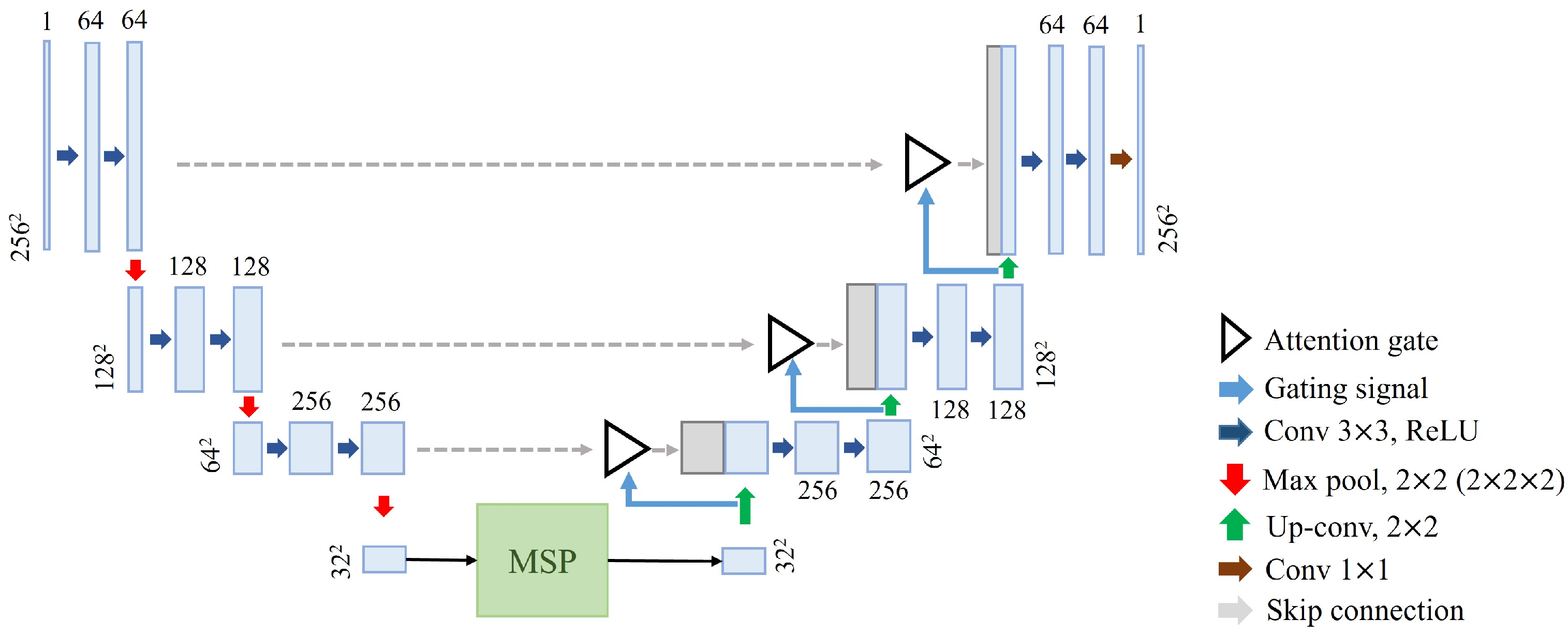
As shown in Figure 4, the WaterSCNet-c was improved from the classic U-Net model [15] by adding an attention gate before the decoder in each of the top three layers and an MSP block between the encoder and the decoder in the bottom layer of the U-shaped encoder and decoder structure. The WaterSCNet-c subnetwork has essentially the same structure as the WaterSCNet-s subnetwork, except that it does not have an MSD path module. The WaterSCNet-c subnetwork does not need the MSD path module because its input is the river segmentation probability maps output from the WaterSCNet-s subnetwork, which do not contain multi-spectral information.
The WaterSCNet-c uses the N × N river probability map output by the WaterSCNet-s as its input. Each value in the river probability map indicates the magnitude of the probability that the segmentation result of the corresponding location in the two-dimensional space belongs to a river.
In the probability map, the probability values corresponding to locations where a river is interrupted by road and bridge crossings differ significantly from those for locations within a river. There are also significant differences in the spatial correlation between the probability values at the true boundaries and breaks of a river and those at other locations around a river.
These differences provide the WaterSCNet-c with essential information for reconstructing river connectivity from the segmentation results of the WaterSCNet-s in an urban environment.
Similar to the WaterSCNet-s, the attention gates in the WaterSCNet-c use gating signals up-sampled from coarse features of the probability map and spatial features extracted from the probability map by the encoder to help reconstruct river connectivity, and the MSP block helps perceive contextual relationships and contextual information of river breaks at multiple spatial scales.

3. Experiments

3.1. Experimental Data

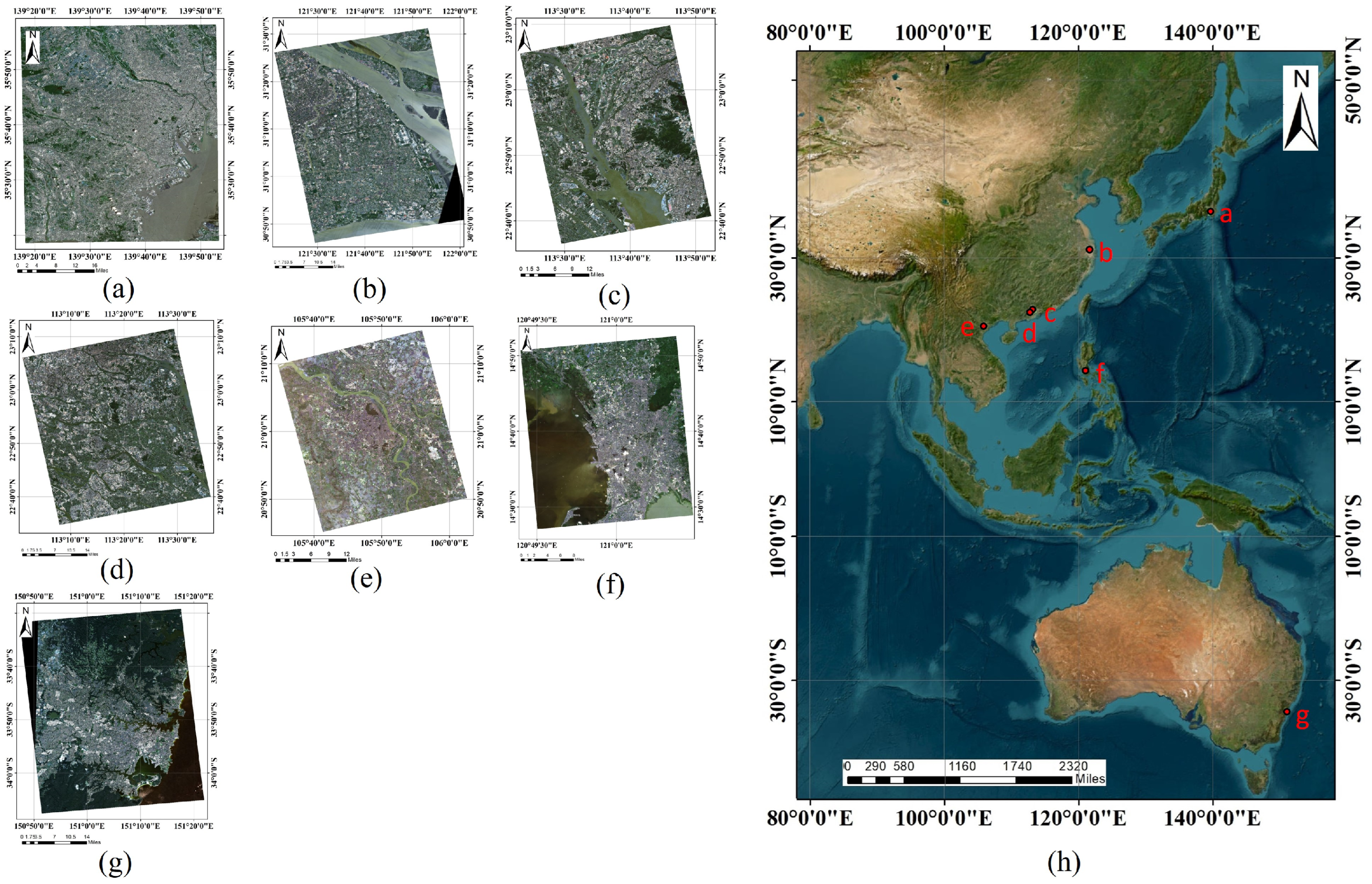
Thirty-nine multi-spectral images of seven cities located in East Asia, Southeast Asia, and Australia were collected from Sentinel-2 Level-2A data products [58] as the source of the experimental data. These images are dated from November 2021 to December 2022.
The Sentinel-2 mission [5] consists of two identical sun-synchronous satellites launched in 2015 and 2017, respectively. Each satellite carries a 13-band Multi-Spectral Instrument (MSI) with spatial resolutions of 10, 20, and 60 m. Sentienal-2 Level-2A (L2A) products consist of 110 × 110 km 2 tiles of radiometrically calibrated and atmospherically corrected surface reflectance imagery [58].
Figure 5 shows the location of the seven cities, which are Tokyo, Shanghai, Dongguan, Guangzhou, Hanoi, Manila, and Sydney. Each city has not only complex river systems, but also well-developed road networks. Therefore, sufficient images of rivers and their interruptions by road and bridge crossings can be collected in these cities to train and evaluate the river segmentation and connectivity reconstruction models.
The multi-spectral images used in this study were selected from the Sentinel-2 L2A data products [58] using the Google Earth Engine [59]. To ensure the quality of the selected images, images with cloud cover greater than 10 % were first filtered out using the quality parameters provided in the Sentinel-2 L2A data products [58], and then images with cloud shadows, snow scenes, and other contamination were excluded based on visual inspection.
The data from the 10th spectral band in the selected images were discarded because they mainly contain information about high-altitude cirrus clouds [60]. To avoid oversmoothing and aliasing, and to preserve spatial detail, the 20 m and 60 m resolution spectral band data in the selected images were interpolated to 10 m resolution using a bi-cubic interpolation technique with the 10 m resolution blue spectral band data as the reference [61].
Figure 6 shows the flowchart of processing, labeling, and slicing of the selected Sentinel-2 data.
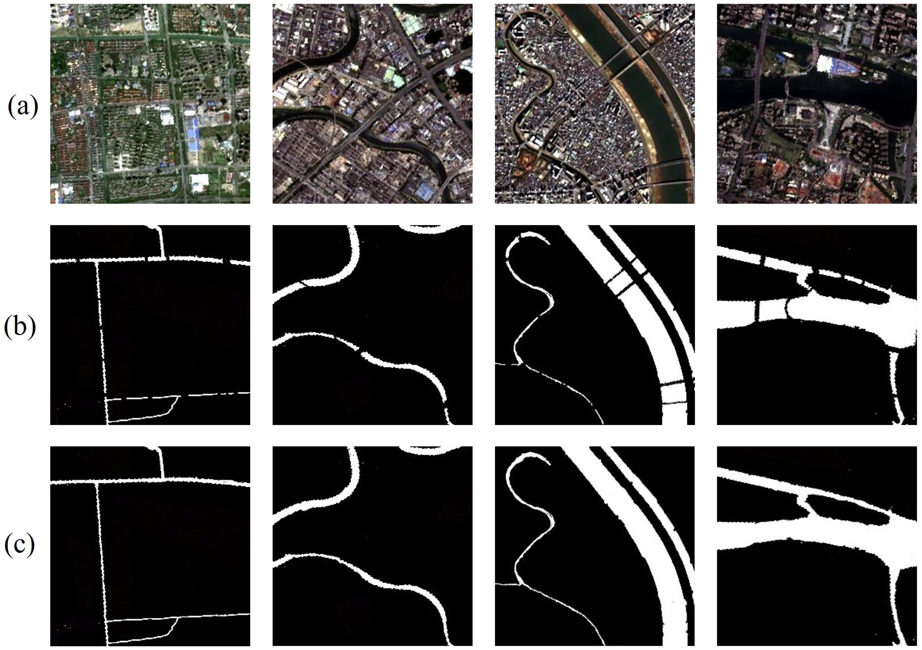
To train, validate, and evaluate the river segmentation and connectivity reconstruction models, the experimental data labels were divided into two types, segmentation labels and connectivity labels, as shown in Figure 7b,c, respectively.
Segmentation labeling was carried out in two steps. River segments were first roughly identified from the collected Sentinel-2 images using the normalized water body index (NDWI) [10] combined with OTSU’s threshold selection method from histograms [62], and then the rough identification results were finely corrected by manual visual comparison with Google Maps to achieve accurate labeling of the river segmentation labels.
Once the segmentation labeling was finished, discontinuities in the segmentation labels caused by road and bridge crossings were visually inspected by comparison with Google Maps, and those verified discontinuities were then manually marked as the connectivity labels.
In the segmentation labels, the smallest river width is 1 pixel, i.e., 10 m. In the connectivity reconstruction labels, the largest and smallest widths of the river discontinuity are 5 pixels and 1 pixel, i.e., 50 m and 10 m, respectively.
The Sentinel-2 multi-spectral images and the corresponding two types of labels were each sliced into 10,614 tiles of size 256 × 256 pixels with an overlap of 10% as the river segmentation dataset and the river connectivity reconstruction dataset for training, validation, and evaluation of the models.

3.2. Model Training

The training process of the WaterSCNet model was divided into two stages, namely the river segmentation stage and river connectivity reconstruction stage, as shown in Figure 8.
In the training stage of river segmentation, Sentinel-2 images and their corresponding river segmentation labels were used as the inputs and training targets for the WaterSCNet-s subnetwork. The trained subnetwork obtained segmentation results based on river segmentation probability feature maps. In the training stage of river connectivity reconstruction, the river segmentation probability feature maps output from the WaterSCNet-s subnetwork and their corresponding connectivity labels were used to train the WaterSCNet-c subnetwork.
The WaterSCNet-s and WaterSCNet-c subnetworks were trained using the Adam stochastic optimization method [63] with an initial learning rate of 0.001, default hyperparameters β 1 of 0.9 and β 2 of 0.999, and a batch size of 4. The threshold of the binarization process during model output was set to 0.5.
The experimental datasets were divided into training, validation, and evaluation datasets according to the ratio of 6:2:2. The training, validation, and evaluation datasets were used to train, validate, and evaluate the WaterSCNet model, respectively.
During the training process, the performance of each subnetwork was evaluated by its validation dataset. If the performance did not improve for five consecutive training epochs, the learning rate was reduced by a factor of 0.5. If the performance did not improve in 50 consecutive training epochs, the training was stopped to prevent the subnetwork from overfitting, and the best performing subnetwork parameters on the evaluation dataset were used as the parameters of the final trained subnetwork.

3.3. Experimental Design

Two types of experiments, training strategy comparison experiments and performance comparison experiments, were conducted in this study.
The WaterSCNet model consists of two subnetworks, the WaterSCNet-s and the WaterSCNet-c. Therefore, two strategies could be used in the training process, namely the synchronous training strategy (experiment Exp_Syn) and the asynchronous training strategy (experiment Exp_Asyn). In the Exp_Asyn, the segmentation subnetwork WaterSCNet-s was first trained, and then the trained WaterSCNet-s was used to generate a set of river segmentation probability maps corresponding to the input multi-spectral images in the training dataset. Each value in the river probability map indicates the magnitude of the probability that the segmentation result of the corresponding pixel in a multi-spectral image input to the segmentation subnetwork belongs to a river. Then, the connectivity reconstruction subnetwork WaterSCNet-c was trained using the river segmentation probability maps as its inputs and the connectivity reconstruction labels as its targets. In the Exp_Syn, the two subnetworks were trained simultaneously.
The network that performed best in the training strategy comparison experiments was used as the final trained WaterSCNet model in the performance comparison experiments.
Just like the training strategy comparison experiments, the performance comparison experiments also contained two parts, which were (1) comparing the river segmentation performance of the WaterSCNet model with commonly used semantic segmentation models such as U-Net [15], SegNet [18], HRNet [19], and E-UNet [17] (experiment Exp_Seg) and (2) comparing the performance of the WaterSCNet model with these commonly used models in river connectivity reconstruction (experiment Exp_Con).
Five groups of training, validation, and evaluation datasets were randomly generated from the experimental datasets to evaluate the robustness of each model in the experiments. Based on these five groups of datasets, both the training strategy comparison experiments and the performance evaluation experiments were independently repeated five times each. The mean and variance of the performance metrics for the five trials were used to represent the final performance and uncertainty of each model, respectively.

3.4. Evaluation Metrics

The Matthews correlation coefficient (MCC), Kappa coefficient, F1 score, and Recall were used as quantitative evaluation metrics to assess the performance of each model in the experiments.
For each tile sample in the validation and evaluation datasets, a confusion matrix was calculated to record the results of comparing the model output with the corresponding label for each pixel in the sample. There were four types of comparison results: true positive (TP), true negative (TN), false positive (FP), and false negative (FN).
Using this confusion matrix, these evaluation metrics could be derived according to Equations (1)–(5). The N in Equation (4) represents the total number of pixels in a tile sample.
P r e c i s i o n = T P T P + F P
R e c a l l = T P T P + F N
F 1 s c o r e = 2 × P r e c i s i o n × R e c a l l P r e c i s o n + R e c a l l
K a p p a c o e f f i c i e n t = N T P + T N T P + F P T P + F N + F N + T N F P + T N N 2 T P + F P T P + F N + F N + T N F P + T N
M C C = T P × T N F P × F N T P + F P T P + F N T N + F P T N + F N

4. Experimental Results and Discussion

4.1. Results of the Training Strategy Comparison Experiments

The performance and uncertainty of the WaterSCNet model in river segmentation and connectivity reconstruction in the training strategy comparison experiments Exp_Syn and Exp_Asyn are listed in Table 2.
The experimental results show that training the two subnetworks in the WaterSCNet model simultaneously yielded slightly better performance in both river segmentation and connectivity reconstruction than training them separately.
Unlike in the Exp_Asyn, where the two subnetworks of the model were optimized separately, in the Exp_Syn the two subnetworks were able to adapt to each other by exchanging feedback information during the optimization process to achieve an overall better performance. Therefore, the models obtained in the simultaneous training strategy experiments (Exp_Syn) were selected for the performance comparison experiments.
The experimental results also show that the variance of all evaluation metrics was very small in the five independent experiments conducted under each training strategy, indicating that the WaterSCNet model had good robustness.

4.2. Results of the Performance Comparison Experiments

Table 3 shows the evaluation results of the river segmentation and connectivity reconstruction performance of the WaterSCNet, E-UNet [17], U-Net [15], SegNet [18], and HRNet [19] models in the performance comparison experiments.
The experimental results show that the WaterSCNet model had the best performance in both river segmentation and connectivity reconstruction compared to the other four models. The WaterSCNet also had the smallest variance in the performance evaluation metrics obtained from the five independent experiments, indicating that it also had the best robustness.
In the river segmentation experiments (Exp_Seg), the MCC, F1, Kappa, and Recall metrics of the WaterSCNet model were 0.925, 0.930, 0.924, and 0.926, respectively, which were better than the classic U-Net model [15] by 3.24%, 3.10%, 3.36%, and 3.93%, and better than the last ranked HRNet model [19] by 5.84%, 5.44%, 5.96%, and 6.56%, respectively.
In the river connectivity reconstruction experiments (Exp_Con), the MCC, F1, Kappa, and Recall metrics of the WaterSCNet model were 0.932, 0.937, 0.931, and 0.933, respectively, outperforming the classic U-Net model [15] by 4.25%, 4.11%, 4.37%, and 4.83%, and outperforming the last ranked HRNet model [19] by 6.03%, 5.64%, 6.16%, and 6.51%, respectively.
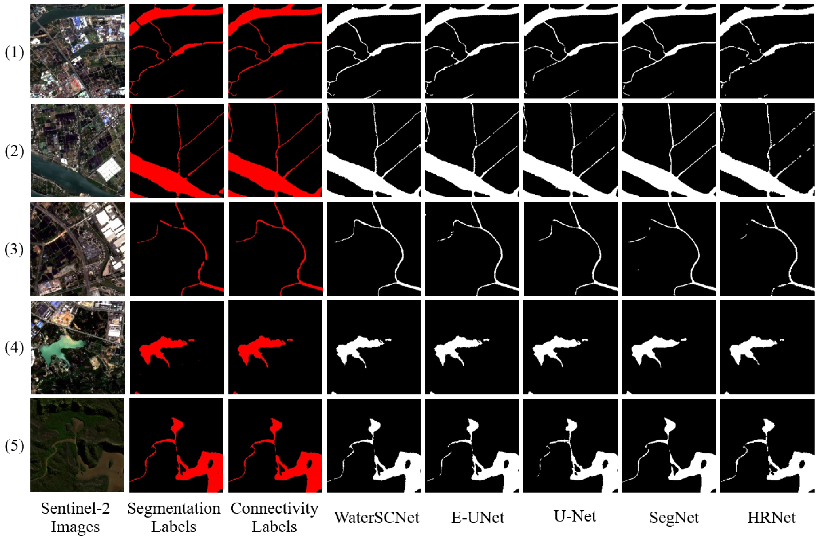
Figure 9 and Figure 10 show examples of the experimental results for river segmentation and connectivity reconstruction, respectively.
The examples in Figure 9 and Figure 10 include experimental results for large, medium, and small rivers in urban areas, urban lakes, and large and small rivers in suburban area, respectively.
Figure 9 shows that all models could achieve roughly equally good segmentation results for large and medium rivers as well as lakes in urban areas. However, as shown in Figure 9(1)–(3), for small rivers, the segmentation results of U-Net, SegNet, and HRNet were obviously inferior to those of WaterSCNet and E-UNet. This is due to the fact that both the river segmentation subnetwork in the WaterSCNet model and the E-UNet model have an MSD path module and an MSP block, which enable them to capture the nonlinear relationship between the multi-spectral bands of adjacent pixels and to perceive the texture relationships and information at multiple spatial scales. Therefore, they were able to achieve better results in segmenting small rivers.
A careful comparison of small river segmentation results of the WaterSCNet model and the E-UNet model in Figure 9(3) shows that the segmentation results of the WaterSCNet model were slightly better. This slight improvement in segmentation performance was due to the addition of the attention gate mechanism in the WaterSCNet-s subnetwork, which can progressively suppress feature responses in irrelevant background regions and help the model focus on regions of interest to achieve better segmentation performance of small rivers from complex urban environments. The smallest river width that can be accurately segmented by the WaterSCNet model is 1 pixel.
Since the number of small rivers in cities is usually much larger than the number of medium and large rivers, the accuracy of small river segmentation is more important for urban river management and biodiversity conservation.
Figure 10 shows that the WaterSCNet model could achieve the best performance in reconstructing the connectivity of small rivers obscured by road and bridge crossings from the segmentation results. This is because, firstly, the WaterSCNet-s subnetwork of the model can achieve the best segmentation performance, providing better river segmentation results for river connectivity reconstruction than the other models; secondly, similar to the WaterSCNet-s subnetwork, the attention gate mechanism added in the WaterSCNet-c subnetwork allows the model to focus on specific regions of river connectivity breaks, resulting in better connectivity reconstruction performance. The WaterSCNet model can accurately reconstruct connectivity breaks up to a maximum width of 5 pixels.
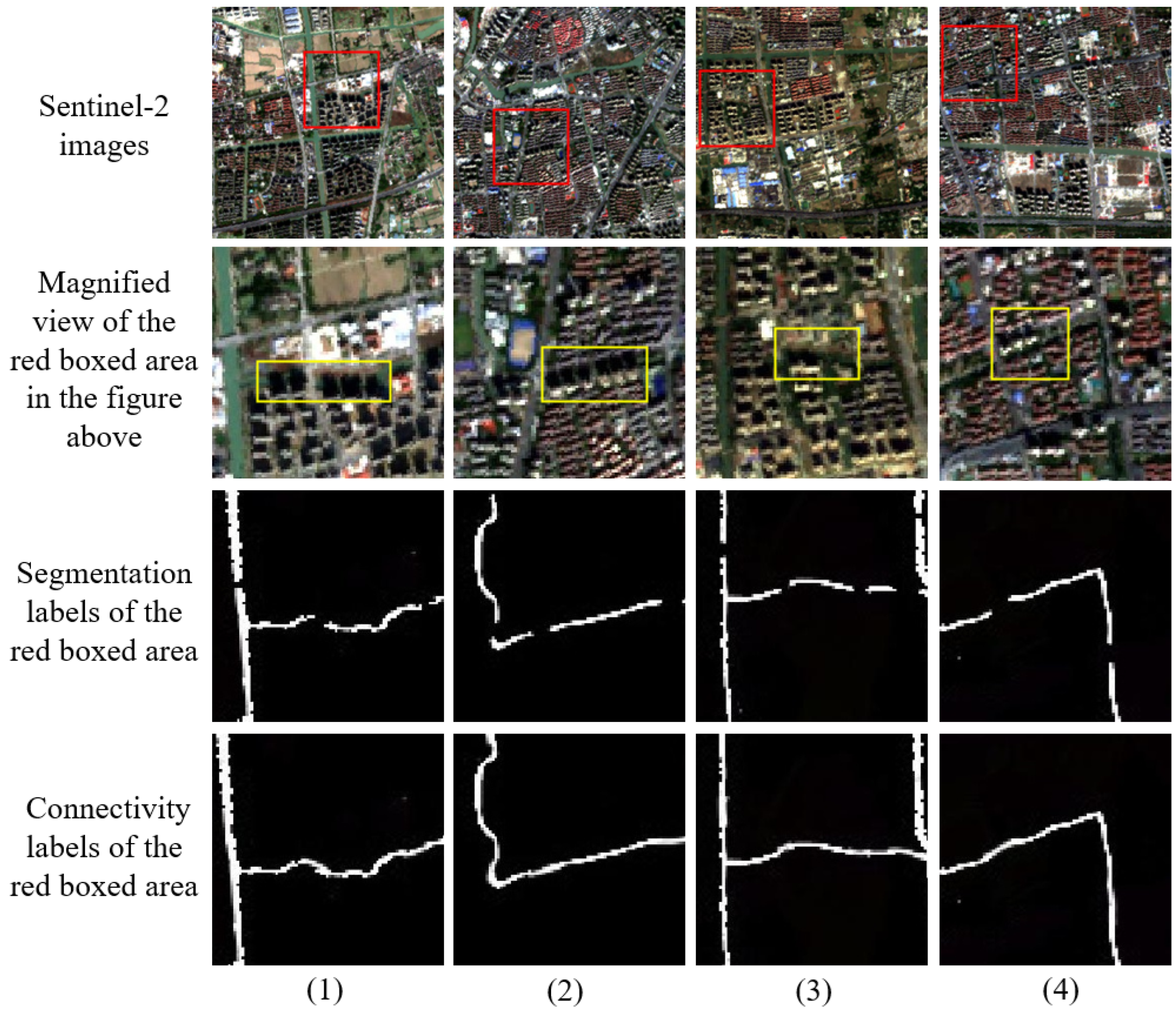
As shown in Figure 11, in dense urban areas, tall buildings may cast shadows on nearby rivers and affect the river segmentation results. The red boxed area in each sub-figure in the first row of Figure 11 indicates the river segment located within the shaded area of nearby tall buildings. The second row of Figure 11 shows the magnified view of these red boxed areas. The shadow of tall buildings in the magnified view is marked by the yellow box. The third and fourth rows of Figure 11 show the segmentation and connectivity labels corresponding to these red boxed areas, respectively.
Figure 12 and Figure 13 show the segmentation and connectivity reconstruction results for the rivers located in the shadow of nearby tall buildings shown in Figure 11. The location of the red box in the segmentation label and connectivity label sub-figures of Figure 12 and Figure 13 is the same as the location of the corresponding red boxed area in the Sentinel-2 images of Figure 11.
Figure 12 shows that all models were able to more or less segment the rivers located within the shadow area of the tall buildings. This is because the multi-spectral information provided by the Sentinel-2 imagery can help the models to mitigate the influence of shadows on the segmentation results. Of all the models, the WaterSCNet model gave the best segmentation results and seemed to be almost unaffected by the shadows. Figure 13 shows that the river connectivity reconstruction results from the WaterSCNet model also appeared to be almost unaffected by the shadows, significantly outperforming the results from the other models.
This study was of urban rivers, so the reconstruction of river connectivity focused on discontinuities caused by road and bridge crossings. However, in addition to roads and bridges, other obstacles such as dams and dry riverbeds can also cause discontinuities in river connectivity. Dams are typically surmounted by roads, and the spectral signature of dams in multi-spectral imagery may be similar to that of bridges or roads crossing rivers. Therefore, the WaterSCNet model in this study should also be able to reconstruct the connectivity of rivers obscured by dams. Dry riverbeds are usually composed of different materials than roads and bridges, and the spectral signature of dry riverbeds may be quite different from that of roads and bridges. Therefore, it may be necessary to retrain the WaterSCNet model by adding dry riverbed data to the training data before the model can be applied to reconstruct the connectivity of rivers obscured by dry riverbeds.

4.3. Comparison of Computational Costs for Model Training

All models in the experiments were trained on a server with two Intel Xeon Gold 5218R CPUs (40 cores in total), 128 GB of RAM, and an NVIDIA Tesla T4 graphics card. The underlying software environment for model training was Python 3.8, Keras 2.2.0, and TensorFlow GPU 1.7.0.
Table 4 lists the training time required for each model in the performance comparison experiments.
The SegNet model [18] required the least amount of training time, only 5.37 h, while the E-UNet model [17] required the most, up to 43.48 h. The WaterSCNet model required 16.42 h, which was 11.37 h and 5.51 h less than that required by the classic U-Net [15] and HNet [19] models, respectively.

5. Conclusions

In this study, a cascaded deep learning network model for river segmentation and connectivity reconstruction, named WaterSCNet, was proposed to segment urban rivers from Sentinel-2 multi-spectral imagery [5] and simultaneously reconstruct their connectivity obscured by road and bridge crossings from the segmentation results.
The WaterSCNet-s subnetwork, which performed river segmentation in the WaterSCNet model, was improved from the E-UNet model ([17]). Compared with the classic U-Net model ([15]), the addition of the MSD path module, the MSP block, and the attention gate mechanism helped the WaterSCNet-s subnetwork to capture the nonlinear relationship between multi-spectral bands of neighboring pixels, to perceive the texture relationship and information at multiple spatial scales, and to obtain the global positional relationship information between the rivers. Therefore, the WaterSCNet model was able to obtain better river segmentation performance.
The WaterSCNet-c subnetwork, which performed river connectivity reconstruction based on the segmentation results in the WaterSCNet model, had the same architecture as the WaterSCNet-s subnetwork, except that it lacked the MSD path module. The MSP block, and the attention gate mechanism in the WaterSCNet-c subnetwork help it to perceive the texture relationship and information at multiple spatial scales, and to obtain the global positional relationship information between the rivers. Therefore, the WaterSCNet model was also able to simultaneously achieve better river connectivity reconstruction performance.
The performance comparison experiments with the E-UNet [17], U-Net [15], SegNet [18], and HRNet [19] models indicated that the WaterSCNet Model not only achieved the best river segmentation and connectivity reconstruction results from Sentinel-2 imagery but also had the best model robustness. The MCC, F1, Kappa, and Recall metrics for river segmentation of the WaterSCNet model were better than the classic U-Net model [15] by 3.24%, 3.10%, 3.36%, and 3.93%, and better than the last ranked HRNet model [19] by 5.84%, 5.44%, 5.96%, and 6.56%, respectively. The MCC, F1, Kappa, and Recall metrics for river connectivity reconstruction of the WaterSCNet model outperformed the classic U-Net model [15] by 4.25%, 4.11%, 4.37%, and 4.83%, and outperformed the last ranked HRNet model [19] by 6.03%, 5.64%, 6.16%, and 6.51%, respectively.
Multi-spectral remote sensing imagery can also be used to retrieval water quality parameters such as concentration of chlorophyll-a [64,65,66], total suspended matter [64,67], dissolved oxygen [68,69,70], and colored dissolved organic matter [68,69]. In the future, by combining the WaterSCNet model with water quality parameter retrieval models, the entire process of identifying urban rivers and retrieving their water quality parameters from Sentinel-2 multi-spectral data can be automated, and furthermore, by using the river connectivity information reconstructed by the WaterSCNet Model, the water quality interactions between urban rivers can also be automatically evaluated.

Author Contributions

Conceptualization, Q.G.; methodology, Z.D. and Q.G.; software, Z.D.; validation, Z.D.; formal analysis, Z.D. and Q.G.; investigation, Z.D. and Q.G.; resources, Q.G.; data curation, Z.D.; writing—original draft preparation, Z.D.; writing—review and editing, Q.G., Y.H., M.W. and J.J.; visualization, Z.D.; supervision, Q.G.; project administration, Z.D.; funding acquisition, Q.G. and M.W. All authors have read and agreed to the published version of the manuscript.

Funding

This research was funded by the National Natural Science Foundation of China, Urban Agglomeration Planning Evaluation Model for Carbon Peaking based on the Multiple Data (project No. 52178060), and the Shanghai Science and Technology Innovation Action Plan 2020, Research on Rapid Detection of River Network Structure and Inversion of Typical Water Quality Parameters Based on Satellite Remote Sensing Imagery (grant No. 20dz1204302), and the DNL Cooperation Fund, Chinese Academy of Sciences (grant numbers DNL202025).

Data Availability Statement

Sentinel-2 data are provided by the European Space Agency (ESA) and available from Copernicus Open Access Hub (https://scihub.copernicus.eu/dhus/#/home, accessed on 8 October 2023) and Google Earth Engine (GEE) (https://earthengine.google.com/, accessed on 8 October 2023). The codes of this study are freely available at https://github.com/ZXDui/WaterSCNet, accessed on 24 September 2023, under the open-source license.

Acknowledgments

The authors wish to thank the ESA/Copernicus and GEE for the freely available data, as well as the Tensorflow and Keras deep learning development platforms used in this study.

Conflicts of Interest

The authors declare no conflict of interest.

References

  1. O’Callaghan, J.F.; Mark, D.M. The extraction of drainage networks from digital elevation data. Comput. Vision Graph. Image Process. 1984, 28, 323–344. [Google Scholar] [CrossRef]
  2. Tarboton, D.G. A new method for the determination of flow directions and upslope areas in grid digital elevation models. Water Resour. Res. 1997, 33, 309–319. [Google Scholar]
  3. Wang, Z.; Liu, J.; Li, J.; Meng, Y.; Pokhrel, Y.; Zhang, H. Basin-scale high-resolution extraction of drainage networks using 10-m Sentinel-2 imagery. Remote Sens. Environ. 2021, 255, 112281. [Google Scholar]
  4. Lu, L.; Wang, L.; Yang, Q.; Zhao, P.; Du, Y.; Xiao, F.; Ling, F. Extracting a Connected River Network from DEM by Incorporating Surface River Occurrence Data and Sentinel-2 Imagery in the Danjiangkou Reservoir Area. Remote Sens. 2023, 15, 1014. [Google Scholar] [CrossRef]
  5. Drusch, M.; Del Bello, U.; Carlier, S.; Colin, O.; Fernandez, V.; Gascon, F.; Hoersch, B.; Isola, C.; Laberinti, P.; Martimort, P.; et al. Sentinel-2: ESA’s optical high-resolution mission for GMES operational services. Remote Sens. Environ. 2012, 120, 25–36. [Google Scholar] [CrossRef]
  6. Grosse, P.; De Vries, B.V.W.; Euillades, P.A.; Kervyn, M.; Petrinovic, I.A. Systematic morphometric characterization of volcanic edifices using digital elevation models. Geomorphology 2012, 136, 114–131. [Google Scholar]
  7. Lashermes, B.; Foufoula-Georgiou, E.; Dietrich, W.E. Channel network extraction from high resolution topography using wavelets. Geophys. Res. Lett. 2007, 34, L23S04. [Google Scholar] [CrossRef]
  8. Yang, K.; Li, M.; Liu, Y.; Cheng, L.; Huang, Q.; Chen, Y. River detection in remotely sensed imagery using Gabor filtering and path opening. Remote Sens. 2015, 7, 8779–8802. [Google Scholar] [CrossRef]
  9. McFeeters, S.K. The use of the Normalized Difference Water Index (NDWI) in the delineation of open water features. Int. J. Remote Sens. 1996, 17, 1425–1432. [Google Scholar] [CrossRef]
  10. Gao, B.C. Normalized difference water index for remote sensing of vegetation liquid water from space. In Proceedings of the Imaging Spectrometry, Orlando, FL, USA, 17–18 April 1995; Volume 2480, pp. 225–236. [Google Scholar]
  11. Xu, H. Modification of normalised difference water index (NDWI) to enhance open water features in remotely sensed imagery. Int. J. Remote Sens. 2006, 27, 3025–3033. [Google Scholar] [CrossRef]
  12. Sghaier, M.O.; Foucher, S.; Lepage, R. River extraction from high-resolution SAR images combining a structural feature set and mathematical morphology. IEEE J. Sel. Top. Appl. Earth Obs. Remote Sens. 2016, 10, 1025–1038. [Google Scholar] [CrossRef]
  13. Fan, Z.; Hou, J.; Zang, Q.; Chen, Y.; Yan, F. River Segmentation of Remote Sensing Images Based on Composite Attention Network. Complexity 2022, 2022, 7750281. [Google Scholar] [CrossRef]
  14. Gu, J.; Wang, Z.; Kuen, J.; Ma, L.; Shahroudy, A.; Shuai, B.; Liu, T.; Wang, X.; Wang, G.; Cai, J.; et al. Recent advances in convolutional neural networks. Pattern Recognit. 2018, 77, 354–377. [Google Scholar]
  15. Ronneberger, O.; Fischer, P.; Brox, T. U-net: Convolutional networks for biomedical image segmentation. In Proceedings of the Medical Image Computing and Computer-Assisted Intervention–MICCAI 2015: 18th International Conference, Munich, Germany, 5–9 October 2015; Springer: Berlin/Heidelberg, Germany, 2015; pp. 234–241. [Google Scholar]
  16. Zhou, Z.; Rahman Siddiquee, M.M.; Tajbakhsh, N.; Liang, J. Unet++: A nested u-net architecture for medical image segmentation. In Proceedings of the Deep Learning in Medical Image Analysis and Multimodal Learning for Clinical Decision Support: 4th International Workshop, DLMIA 2018, and 8th International Workshop, ML-CDS 2018, Held in Conjunction with MICCAI 2018, Granada, Spain, 20 September 2018; Springer: Berlin/Heidelberg, Germany, 2018; pp. 3–11. [Google Scholar]
  17. Dui, Z.; Huang, Y.; Jin, J.; Gu, Q. Automatic detection of photovoltaic facilities from Sentinel-2 observations by the enhanced U-Net method. J. Appl. Remote Sens. 2023, 17, 014516. [Google Scholar] [CrossRef]
  18. Badrinarayanan, V.; Kendall, A.; Cipolla, R. Segnet: A deep convolutional encoder–decoder architecture for image segmentation. IEEE Trans. Pattern Anal. Mach. Intell. 2017, 39, 2481–2495. [Google Scholar] [CrossRef] [PubMed]
  19. Sun, K.; Xiao, B.; Liu, D.; Wang, J. Deep high-resolution representation learning for human pose estimation. In Proceedings of the IEEE/CVF Conference on Computer Vision and Pattern Recognition, Long Beach, CA, USA, 15–20 June 2019; pp. 5693–5703. [Google Scholar]
  20. Zhu, X.X.; Tuia, D.; Mou, L.; Xia, G.S.; Zhang, L.; Xu, F.; Fraundorfer, F. Deep learning in remote sensing: A comprehensive review and list of resources. IEEE Geosci. Remote Sens. Mag. 2017, 5, 8–36. [Google Scholar] [CrossRef]
  21. Wei, S.; Zhang, H.; Wang, C.; Wang, Y.; Xu, L. Multi-temporal SAR data large-scale crop mapping based on U-Net model. Remote Sens. 2019, 11, 68. [Google Scholar] [CrossRef]
  22. Abderrahim, N.Y.Q.; Abderrahim, S.; Rida, A. Road segmentation using u-net architecture. In Proceedings of the 2020 IEEE International Conference of Moroccan Geomatics (Morgeo), Casablanca, Morocco, 11–13 May 2020; pp. 1–4. [Google Scholar]
  23. Chen, C.; Fan, L. Scene segmentation of remotely sensed images with data augmentation using U-net++. In Proceedings of the 2021 International Conference on Computer Engineering and Artificial Intelligence (ICCEAI), Shanghai, China, 27–29 August 2021; pp. 201–205. [Google Scholar]
  24. Ji, S.; Zhang, C.; Xu, A.; Shi, Y.; Duan, Y. 3D convolutional neural networks for crop classification with multi-temporal remote sensing images. Remote Sens. 2018, 10, 75. [Google Scholar] [CrossRef]
  25. Palsson, F.; Sveinsson, J.R.; Ulfarsson, M.O. Multispectral and hyperspectral image fusion using a 3-D-convolutional neural network. IEEE Geosci. Remote Sens. Lett. 2017, 14, 639–643. [Google Scholar] [CrossRef]
  26. Chen, Y.; Jiang, H.; Li, C.; Jia, X.; Ghamisi, P. Deep feature extraction and classification of hyperspectral images based on convolutional neural networks. IEEE Trans. Geosci. Remote Sens. 2016, 54, 6232–6251. [Google Scholar] [CrossRef]
  27. Cao, Z.; Li, X.; Jianfeng, J.; Zhao, L. 3D convolutional siamese network for few-shot hyperspectral classification. J. Appl. Remote Sens. 2020, 14, 048504. [Google Scholar] [CrossRef]
  28. Yoo, D.; Park, S.; Lee, J.Y.; Kweon, I.S. Multi-scale pyramid pooling for deep convolutional representation. In Proceedings of the 2015 IEEE Conference on Computer Vision and Pattern Recognition Workshops (CVPRW), Boston, MA, USA, 7–12 June 2015; pp. 71–80. [Google Scholar] [CrossRef]
  29. Miao, Z.; Fu, K.; Sun, H.; Sun, X.; Yan, M. Automatic water-body segmentation from high-resolution satellite images via deep networks. IEEE Geosci. Remote Sens. Lett. 2018, 15, 602–606. [Google Scholar] [CrossRef]
  30. Chen, Y.; Fan, R.; Yang, X.; Wang, J.; Latif, A. Extraction of urban water bodies from high-resolution remote-sensing imagery using deep learning. Water 2018, 10, 585. [Google Scholar] [CrossRef]
  31. Li, M.; Pan, T.; Guan, H.; Liu, H.; Gao, J. Gaofen-2 mission introduction and characteristics. In Proceedings of the 66th International Astronautical Congress (IAC 2015), Jerusalem, Israel, 12–16 October 2015; pp. 12–16. [Google Scholar]
  32. Xu, R.; Liu, J.; Xu, J. Extraction of high-precision urban impervious surfaces from sentinel-2 multispectral imagery via modified linear spectral mixture analysis. Sensors 2018, 18, 2873. [Google Scholar] [CrossRef] [PubMed]
  33. Liu, C.C.; Zhang, Y.C.; Chen, P.Y.; Lai, C.C.; Chen, Y.H.; Cheng, J.H.; Ko, M.H. Clouds classification from Sentinel-2 imagery with deep residual learning and semantic image segmentation. Remote Sens. 2019, 11, 119. [Google Scholar] [CrossRef]
  34. Zhang, Y. A method for continuous extraction of multispectrally classified urban rivers. Photogramm. Eng. Remote Sens. 2000, 66, 991–999. [Google Scholar]
  35. Li, X.; Lyu, X.; Tong, Y.; Li, S.; Liu, D. An object-based river extraction method via optimized transductive support vector machine for multi-spectral remote-sensing images. IEEE Access 2019, 7, 46165–46175. [Google Scholar] [CrossRef]
  36. Yuan, K.; Zhuang, X.; Schaefer, G.; Feng, J.; Guan, L.; Fang, H. Deep-learning-based multispectral satellite image segmentation for water body detection. IEEE J. Sel. Top. Appl. Earth Obs. Remote Sens. 2021, 14, 7422–7434. [Google Scholar] [CrossRef]
  37. Isikdogan, F.; Bovik, A.C.; Passalacqua, P. Surface water mapping by deep learning. IEEE J. Sel. Top. Appl. Earth Obs. Remote Sens. 2017, 10, 4909–4918. [Google Scholar] [CrossRef]
  38. Gutman, G.; Byrnes, R.A.; Masek, J.G.; Covington, S.; Justice, C.O.; Franks, S.; Headley, R.M.K. Towards monitoring land-cover and land-use changes at a global scale: The global land survey 2005. Photogramm. Eng. Remote Sens. 2008, 74, 6–10. [Google Scholar]
  39. Jiang, W.; He, G.; Long, T.; Ni, Y. Detecting water bodies in landsat8 oli image using deep learning. Int. Arch. Photogramm. Remote Sens. Spat. Inf. Sci 2018, 42, 669–672. [Google Scholar] [CrossRef]
  40. Hornik, K.; Stinchcombe, M.; White, H. Multilayer feedforward networks are universal approximators. Neural Netw. 1989, 2, 359–366. [Google Scholar] [CrossRef]
  41. Roy, D.P.; Wulder, M.A.; Loveland, T.R.; Woodcock, C.E.; Allen, R.G.; Anderson, M.C.; Helder, D.; Irons, J.R.; Johnson, D.M.; Kennedy, R.; et al. Landsat-8: Science and product vision for terrestrial global change research. Remote Sens. Environ. 2014, 145, 154–172. [Google Scholar]
  42. Xia, M.; Qian, J.; Zhang, X.; Liu, J.; Xu, Y. River segmentation based on separable attention residual network. J. Appl. Remote Sens. 2020, 14, 032602. [Google Scholar] [CrossRef]
  43. Lin, Q.; Han, Y.; Hahn, H. Real-time lane departure detection based on extended edge-linking algorithm. In Proceedings of the 2010 Second International Conference on Computer Research and Development, Kuala Lumpur, Malaysia, 7–10 May 2010; pp. 725–730. [Google Scholar]
  44. Yu, J.; Han, Y.; Hahn, H. An efficient extraction of on-road object and lane information using representation method. In Proceedings of the 2008 IEEE International Conference on Signal Image Technology and Internet Based Systems, Bali, Indonesia, 30 November–3 December 2008; pp. 327–332. [Google Scholar]
  45. Oktay, O.; Schlemper, J.; Folgoc, L.L.; Lee, M.; Heinrich, M.; Misawa, K.; Mori, K.; McDonagh, S.; Hammerla, N.Y.; Kainz, B.; et al. Attention u-net: Learning where to look for the pancreas. arXiv 2018, arXiv:1804.03999. [Google Scholar]
  46. Hu, J.; Shen, L.; Sun, G. Squeeze-and-excitation networks. In Proceedings of the IEEE Conference on Computer Vision and Pattern Recognition, Salt Lake City, UT, USA, 18–23 June 2018; pp. 7132–7141. [Google Scholar]
  47. Hu, J.; Shen, L.; Albanie, S.; Sun, G.; Vedaldi, A. Gather-excite: Exploiting feature context in convolutional neural networks. Adv. Neural Inf. Process. Syst. 2018, 31, 1–11. [Google Scholar]
  48. Woo, S.; Park, J.; Lee, J.Y.; Kweon, I.S. Cbam: Convolutional block attention module. In Proceedings of the European Conference on Computer Vision (ECCV), Munich, Germany, 8–14 September 2018; pp. 3–19. [Google Scholar]
  49. Schlemper, J.; Oktay, O.; Schaap, M.; Heinrich, M.; Kainz, B.; Glocker, B.; Rueckert, D. Attention gated networks: Learning to leverage salient regions in medical images. Med. Image Anal. 2019, 53, 197–207. [Google Scholar] [CrossRef]
  50. Zhao, B.; Feng, J.; Wu, X.; Yan, S. A survey on deep learning-based fine-grained object classification and semantic segmentation. Int. J. Autom. Comput. 2017, 14, 119–135. [Google Scholar] [CrossRef]
  51. Mnih, V.; Heess, N.; Graves, A. Recurrent models of visual attention. Adv. Neural Inf. Process. Syst. 2014, 27, 1–9. [Google Scholar]
  52. Bahdanau, D.; Cho, K.; Bengio, Y. Neural machine translation by jointly learning to align and translate. arXiv 2014, arXiv:1409.0473. [Google Scholar]
  53. Britz, D.; Goldie, A.; Luong, M.T.; Le, Q. Massive exploration of neural machine translation architectures. arXiv 2017, arXiv:1703.03906. [Google Scholar]
  54. Glorot, X.; Bordes, A.; Bengio, Y. Deep sparse rectifier neural networks. In Proceedings of the 14th International Conference on Artificial Intelligence and Statistics. JMLR Workshop and Conference Proceedings, Fort Lauderdale, FL, USA, 11–13 April 2011; pp. 315–323. [Google Scholar]
  55. Han, J.; Moraga, C. The influence of the sigmoid function parameters on the speed of backpropagation learning. In Proceedings of the From Natural to Artificial Neural Computation: International Workshop on Artificial Neural Networks, Malaga-Torremolinos, Spain, 7–9 June 1995; Proceedings 3. Springer: Berlin/Heidelberg, Germany, 1995; pp. 195–201. [Google Scholar]
  56. Jiang, C.; Zhang, H.; Wang, C.; Ge, J.; Wu, F. Water Surface Mapping from Sentinel-1 Imagery Based on Attention-UNet3+: A Case Study of Poyang Lake Region. Remote Sens. 2022, 14, 4708. [Google Scholar] [CrossRef]
  57. Mnih, V.; Heess, N.; Graves, A.; Kavukcuoglu, K. Recurrent Models of Visual Attention. In Proceedings of the Advances in Neural Information Processing Systems, Montreal, QC, Canada, 8–13 December 2014; Volume 27. [Google Scholar]
  58. Muller-Wilm, U.; Louis, J.; Richter, R.; Gascon, F.; Niezette, M. Sentinel-2 level 2A prototype processor: Architecture, algorithms and first results. In Proceedings of the ESA Living Planet Symposium, Edinburgh, UK, 9–13 September 2013; pp. 9–13. [Google Scholar]
  59. Gorelick, N.; Hancher, M.; Dixon, M.; Ilyushchenko, S.; Thau, D.; Moore, R. Google Earth Engine: Planetary-scale geospatial analysis for everyone. Remote Sens. Environ. 2017, 202, 18–27. [Google Scholar] [CrossRef]
  60. Li, H.; Wang, C.; Cui, Y.; Hodgson, M. Mapping salt marsh along coastal South Carolina using U-Net. ISPRS J. Photogramm. Remote Sens. 2021, 179, 121–132. [Google Scholar] [CrossRef]
  61. Liu, C.; Huang, H.; Hui, F.; Zhang, Z.; Cheng, X. Fine-resolution mapping of pan-arctic lake ice-off phenology based on dense sentinel-2 time series data. Remote Sens. 2021, 13, 2742. [Google Scholar] [CrossRef]
  62. Otsu, N. A threshold selection method from gray-level histograms. IEEE Trans. Syst. Man Cybern. 1979, 9, 62–66. [Google Scholar] [CrossRef]
  63. Kingma, D.P.; Ba, J. Adam: A method for stochastic optimization. arXiv 2014, arXiv:1412.6980. [Google Scholar]
  64. Niroumand-Jadidi, M.; Bovolo, F.; Bresciani, M.; Gege, P.; Giardino, C. Water Quality Retrieval from Landsat-9 (OLI-2) Imagery and Comparison to Sentinel-2. Remote Sens. 2022, 14, 4596. [Google Scholar] [CrossRef]
  65. Niroumand-Jadidi, M.; Bovolo, F.; Bruzzone, L.; Gege, P. Inter-Comparison of Methods for Chlorophyll-a Retrieval: Sentinel-2 Time-Series Analysis in Italian Lakes. Remote Sens. 2021, 13, 2381. [Google Scholar] [CrossRef]
  66. Ansper, A.; Alikas, K. Retrieval of Chlorophyll a from Sentinel-2 MSI Data for the European Union Water Framework Directive Reporting Purposes. Remote Sens. 2019, 11, 64. [Google Scholar] [CrossRef]
  67. Ciancia, E.; Campanelli, A.; Lacava, T.; Palombo, A.; Pascucci, S.; Pergola, N.; Pignatti, S.; Satriano, V.; Tramutoli, V. Modeling and Multi-Temporal Characterization of Total Suspended Matter by the Combined Use of Sentinel 2-MSI and Landsat 8-OLI Data: The Pertusillo Lake Case Study (Italy). Remote Sens. 2020, 12, 2147. [Google Scholar] [CrossRef]
  68. Sent, G.; Biguino, B.; Favareto, L.; Cruz, J.; Sá, C.; Dogliotti, A.I.; Palma, C.; Brotas, V.; Brito, A.C. Deriving Water Quality Parameters Using Sentinel-2 Imagery: A Case Study in the Sado Estuary, Portugal. Remote Sens. 2021, 13, 1043. [Google Scholar] [CrossRef]
  69. Virdis, S.G.; Xue, W.; Winijkul, E.; Nitivattananon, V.; Punpukdee, P. Remote sensing of tropical riverine water quality using sentinel-2 MSI and field observations. Ecol. Indic. 2022, 144, 109472. [Google Scholar] [CrossRef]
  70. Peterson, K.T.; Sagan, V.; Sloan, J.J. Deep learning-based water quality estimation and anomaly detection using Landsat-8/Sentinel-2 virtual constellation and cloud computing. Gisci. Remote Sens. 2020, 57, 510–525. [Google Scholar] [CrossRef]
Figure 1. Top-level architecture of the WaterSCNet model.
Remotesensing 15 04875 g001
Figure 2. Architecture of the river segmentation subnetwork WaterSCNet-s.
Remotesensing 15 04875 g002
Figure 3. Schematic of the additive attention gate.
Remotesensing 15 04875 g003
Figure 4. Architecture of the river network connectivity reconstruction subnetwork: WaterSCNet-c.
Remotesensing 15 04875 g004
Figure 5. Sentinel-2 multi-spectral image of the seven cities, (a) Tokyo, (b) Shanghai, (c) Dongguan, (d) Guangzhou, (e) Hanoi, (f) Manila, (g) Sydney, (h) location of the seven cities (https://services.arcgisonline.com/arcgis/rest/services, accessed on 25 July 2023).
Remotesensing 15 04875 g005
Figure 6. Sentinel-2 data processing, labeling, and slicing flowchart.
Remotesensing 15 04875 g006
Figure 7. Examples of river segmentation labels and river connectivity reconstruction labels, (a) sentinel-2 images, (b) river segmentation labels, (c) river connectivity reconstruction labels.
Remotesensing 15 04875 g007
Figure 8. Schematic of the training process of the WaterSCNet model, a river segmentation and connectivity reconstruction network.
Remotesensing 15 04875 g008
Figure 9. Examples of experimental results for river segmentation (Exp_Seg), (1) medium and small urban rivers, (2) large and small urban rivers, (3) small urban rivers, (4) urban lakes, (5) large and small suburban rivers.
Remotesensing 15 04875 g009
Figure 10. Examples of experimental results for river connectivity reconstruction (Exp_Con), (1) medium and small urban rivers, (2) large and small urban rivers, (3) small urban rivers, (4) urban lakes, (5) large and small suburban rivers.
Remotesensing 15 04875 g010
Figure 11. Examples of rivers located within the shaded area of nearby tall buildings, and their segmentation and connectivity labels. (14) are four examples, the red boxes indicate the river segment located within the shadow of nearby tall buildings, the yellow boxes indicate the shadow of tall buildings.
Remotesensing 15 04875 g011
Figure 12. Segmentation results for the rivers located in the shaded area of nearby tall buildings in Figure 11. (14) correspond to the four examples in Figure 11, the red boxes indicate the same location as the corresponding red boxed areas in the Sentinel-2 images of Figure 11.
Remotesensing 15 04875 g012
Figure 13. Connectivity reconstruction results for the rivers located in the shaded area of nearby tall buildings in Figure 11. (14) correspond to the four examples in Figure 11, the red boxes indicate the same location as the corresponding red boxed areas in the Sentinel-2 images of Figure 11.
Remotesensing 15 04875 g013
Table 1. Parameters of the MSD path module.
Layer NameLayer Input(Filter Size) × NumberOutput Size
C1Input(5 × 5 × 5) × 32(256 × 256 × 12) × 32
R1C1-256 × 256 × 384
C2R1(1 × 1) × 16256 × 256 × 16
P1C12 × 2 × 2(128 × 128 × 6) × 32
C3P1(5 × 5 × 5) × 64(128 × 128 × 6) × 64
R2C3-128 × 128 × 384
C4R2(1 × 1) × 32128 × 128 × 32
P2C32 × 2 × 2(64 × 64 × 3) × 64
C5P2(5 × 5 × 5) × 128(64 × 64 × 3) × 128
R3C5-64 × 64 × 384
C6R3(1 × 1) × 6464 × 64 × 64
Table 2. Experimental results of the training strategy comparison experiments.
Evaluation
Subject
ExperimentEvaluation Results
MCCF1KappaRecall
RiverExp_Syn0.925 ± 0.0050.930 ± 0.0050.924 ± 0.0050.926 ± 0.005
SegmentationExp_Asyn0.926 ± 0.0040.931 ± 0.0030.925 ± 0.0040.928 ± 0.005
River connectivityExp_Syn0.932 ± 0.0030.937 ± 0.0030.931 ± 0.0030.933 ± 0.005
reconstructionExp_Asyn0.928 ± 0.0040.933 ± 0.0030.927 ± 0.0040.929 ± 0.002
Table 3. Experimental results of the performance comparison experiments.
ExperimentModelEvaluation Results
MCCF1KappaRecall
Exp_SegWaterSCNet0.925 ± 0.0050.930 ± 0.0050.924 ± 0.0050.926 ± 0.005
E-UNet0.915 ± 0.0090.921 ± 0.0090.914 ± 0.0090.916 ± 0.013
U-Net0.896 ± 0.0140.902 ± 0.0140.894 ± 0.0150.891 ± 0.020
SegNet0.879 ± 0.0120.886 ± 0.0120.876 ± 0.0130.869 ± 0.018
HRNet0.874 ± 0.0040.882 ± 0.0040.872 ± 0.0050.869 ± 0.007
Exp_ConWaterSCNet0.932 ± 0.0030.937 ± 0.0030.931 ± 0.0030.933 ± 0.005
E-UNet0.906 ± 0.0100.912 ± 0.0100.904 ± 0.0110.905 ± 0.011
U-Net0.894 ± 0.0100.900 ± 0.0100.892 ± 0.0110.890 ± 0.014
SegNet0.883 ± 0.0060.891 ± 0.0050.881 ± 0.0060.878 ± 0.003
HRNet0.879 ± 0.0060.887 ± 0.0060.877 ± 0.0060.876 ± 0.009
Table 4. Model training time for river segmentation (Exp_Seg) and connectivity reconstruction (Exp_Con) experiments.
ExperimentModel Training Time (Hours of CPU Time)
WaterSCNetE-UNetU-NetSegNetHRNet
Exp_Seg16.42 122.1615.072.9612.56
Exp_Con21.3212.722.419.37
Total16.4243.4827.795.3721.93
1 The two subnetworks of river segmentation and connectivity reconstruction in the WaterSCNet model were trained simultaneously.
Disclaimer/Publisher’s Note: The statements, opinions and data contained in all publications are solely those of the individual author(s) and contributor(s) and not of MDPI and/or the editor(s). MDPI and/or the editor(s) disclaim responsibility for any injury to people or property resulting from any ideas, methods, instructions or products referred to in the content.