Abstract
Nanosatellites are proliferating as low-cost, dedicated remote sensing opportunities for small nations. However, nanosatellites’ performance as remote sensing platforms is impaired by low downlink speeds, which typically range from 1200 to 9600 bps. Additionally, an estimated 67% of downloaded data are unusable for further applications due to excess cloud cover. To alleviate this issue, we propose an image segmentation and prioritization algorithm to classify and segment the contents of captured images onboard the nanosatellite. This algorithm prioritizes images with clear captures of water bodies and vegetated areas with high downlink priority. This in-orbit organization of images will aid ground station operators with downlinking images suitable for further ground-based remote sensing analysis. The proposed algorithm uses Convolutional Neural Network (CNN) models to classify and segment captured image data. In this study, we compare various model architectures and backbone designs for segmentation and assess their performance. The models are trained on a dataset that simulates captured data from nanosatellites and transferred to the satellite hardware to conduct inferences. Ground testing for the satellite has achieved a peak Mean IoU of 75% and an F1 Score of 0.85 for multi-class segmentation. The proposed algorithm is expected to improve data budget downlink efficiency by up to 42% based on validation testing.
1. Introduction
A CubeSat is a small, standardized nanosatellite with a mass ranging from 1 to 10 kg, and it is often used for research and academic purposes. CubeSats are constructed to adhere to specific dimensions known as CubeSat Units or “U”, measuring 10 by 10 by 10 cm, and are officially categorized based on their size as 1U, 2U, 3U, or 6U [1]. Their rising popularity stems from their affordability, compact size, and ease of deployment, making them accessible to both researchers and private enterprises. CubeSats are frequently employed in educational and research endeavors and offer a cost-effective alternative to larger, conventional satellites [2,3,4]. They are designed to be modular, facilitating seamless integration and rapid launch. These miniature satellites can be outfitted with sensors and imaging systems capable of capturing high-resolution Earth surface imagery, enabling the in-depth analysis and categorization of various land cover types and environmental features. Nanosatellites provide a cost-efficient and adaptable platform for a wide spectrum of space-based applications, granting researchers and organizations access to space-based data and services that were previously unattainable [5].
Despite the advantages offered by CubeSats, they are not without limitations, some of which can significantly affect their performance in missions. The most prominent drawbacks are associated with their compact size and weight restrictions. Due to their small form factor, CubeSats have limited payload/bus capacity, which in turn constrains their ability to carry more advanced electronics and scientific instruments. This limitation has a direct impact on the computational power and onboard storage capacity available for data processing and analysis during missions. Furthermore, the diminutive size of CubeSats also influences their communication capabilities. With a constrained surface area available for communication systems and antennas, CubeSats encounter difficulties in maintaining robust and dependable communication links with ground stations. Consequently, data transmission rates may be compromised, and the volume of data that can be relayed to ground stations may be restricted. Based on data collected from the SatNogs Database [6], Figure 1 illustrates that more than 75% of active nanosatellites typically operate within the 20–30 MHz (HF) to 900–980 MHz (UHF) frequency range. These frequency bands are typically chosen due to their robust propagation characteristics and ease of implementation regarding ground station equipment costs. However, these frequency bands have limited bandwidth, which consequently limits the maximum downlink speed capability for these satellites as compared to higher frequency ranges. Only 25% of active nanosatellites operate within the higher frequency bands, such as the S-band (2.2–3.4 GHz), C-band (4–8 GHz), X-Band (8–12 GHz), and K band (18–27 GHz). In these bands, satellites can achieve increased data transfer rates due to the broader bandwidth available. Moreover, these bands often experience less interference, providing a more reliable and efficient communication environment. Additionally, the shorter wavelengths associated with higher frequency bands allow the design of smaller directional antennas, contributing to the development of compact and precise communication systems. Furthermore, the modulation scheme used for communication between the satellite and ground station also significantly affects the achievable downlink rates. Figure 2 shows that the vast majority (73%) of nanosatellites communicate using Gaussian minimum-shift keying (GMSK), binary phase-shift keying (BPSK), frequency-shift keying (FSK), audio frequency-shift keying (AFSK) and gaussian frequency-shift keying (GFSK). These traditional modes of communication are excellent for establishing reliable and efficient communication links in the context of nanosatellite missions. However, these modes have limited capacity for increased data communication. The most commonly achieved baud rate for satellites within each modulation scheme ranges between 1200 and 9600 bps. This implies a maximum data downlink speed ranging between 0.15 and 1.2 KB/s. The typical nanosatellite in a low earth orbit at 500 km achieves a revisit frequency of three passes per day. The average lifespan of nanosatellites is typically 1.1 years [7]. With this time, the theoretical data budget for nanosatellites ranges between 18MB to 145MB with continuous downlink operations. Factors such as operator availability, lost packets, signal interference, weather conditions, and frequency interference can severely impact the downlink process, which reduces this data budget significantly. Depending on the mission and its payload specifications, these budget allocations may be constrained, and the satellite may not meet mission success milestones.
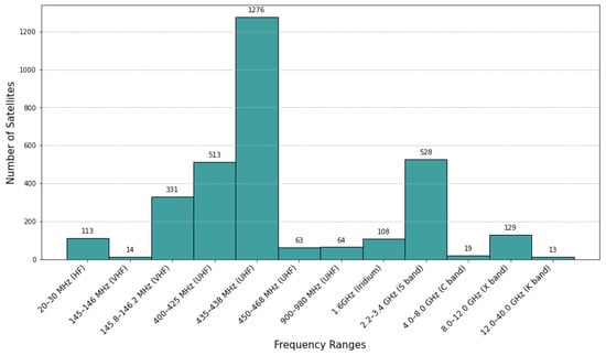
Figure 1.
Number of active nanosatellites and their operating frequency ranges.
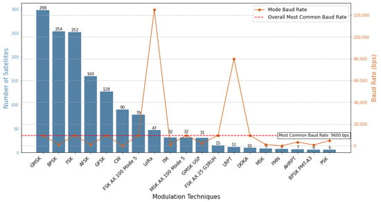
Figure 2.
Distribution of nanosatellites and their modulation modes and the most commonly achievable operating downlink speeds.
In the context of land use and land cover assessment, identifying vegetated lands aids in understanding areas with agricultural activities and forests. Also, pinpointing non-vegetated lands helps identify urbanized areas or barren lands. Additionally, the detection of water bodies further contributes to comprehensive water quality assessment, enabling the monitoring of aquatic ecosystems, pollution sources, and overall environmental health. Combining these analyses provides a holistic understanding of the landscape and supports informed decision-making for sustainable land and water resource management. Water bodies are essential resources for nations and represent important features in remote sensing applications. Detecting and extracting these features is important for monitoring the status of these indispensable natural resources. The study of water bodies uses various technologies and sensors to observe, monitor, and analyze bodies of water on Earth, such as lakes, rivers, oceans, reservoirs, and wetlands [8]. Nanosatellites can detect and monitor water bodies by taking advantage of their low cost and modular design. They can be equipped with a variety of sensors to detect and monitor changes in water resources [9,10,11]. One of the advantages of using satellites for water detection is their ability to cover large areas quickly and frequently, providing up-to-date information on changes in water resources over time. This can be especially useful in detecting changes in water availability due to drought or climate change, as well as monitoring the effects of activities such as irrigation and industrial activities. Nanosatellites can also be deployed in constellations, providing the advantage of frequent revisits to areas of interest. Additionally, CubeSats can swiftly identify and respond to sudden environmental developments, such as the impact of activities like irrigation and industrial processes [10]. There are several techniques commonly used for remote sensing image data, and the most common approaches involve the implementation of segmentation using machine learning techniques. In the paper by [12], a variation of the Pyramid Spatial Pooling (PSPNet) [13] architecture was implemented for urban land image segmentation. The model achieved a 75.4% Mean Intersection of Union (mIoU) on the test dataset. Based on this study, the PSPNet is a viable candidate for testing due to its robust performance and lightweight design. Xiaofei [14] proposed an image segmentation model based on LinkNet [15] for daytime sea fog detection that leverages residual blocks to encoder feature maps and attention modules to learn the features of sea fog data by considering spectral and spatial information of nodes. This paper demonstrates the performance of LinkNet and its variations on limited datasets and achieves a critical success index (CSI) of 80%.
Cloud cover estimation in remote sensing is a critical aspect of satellite-based observations. In regions characterized by a high cloud fraction, the downlink constraint of nanosatellites poses a significant challenge for remote sensing applications, particularly in the retrieval of clear images when limited downloads are available. A prior study [16] indicated that around 67% of land is obscured by clouds, with localized areas experiencing cloud fractions exceeding 80%. This suggests that, depending on the specific region, there is a considerable likelihood that images received via downlink may encompass cloudy scenes, thereby diminishing the effective downlink capacity of nanosatellites. Cloud cover estimation involves assessing the extent to which clouds obscure the Earth’s surface in images captured by satellites or aerial sensors. Various methods are employed for accurate estimation, including reflectance-based analysis, thermal infrared imaging, multispectral analysis, texture analysis, and advanced techniques like machine learning. By examining spectral characteristics, temperature variations, and spatial patterns and utilizing artificial intelligence, these methods help distinguish clouds from clear areas. Timely and precise cloud cover estimation is vital for applications such as weather forecasting, agriculture, and environmental monitoring. Techniques often involve a combination of these approaches to enhance accuracy and provide valuable insights into atmospheric conditions and land surface characteristics. The current state-of-the-art implementations involve pixel-wise image segmentation using Convolutional Neural Networks (CNNs) [17,18,19]. In work by Drönner [17], a modified version of the U-Net Architecture [20], termed CS-CNN (Cloud Segmentation CNN), was introduced. This modification involved a reduction in the number of kernels, the incorporation of pooling layers using convolution layers with strides, and the addition of dropout layers. These adjustments aimed to streamline computational efficiency, enable the learning of layer-specific downsampling operations, and mitigate overfitting, respectively. The effectiveness of CS-CNN was assessed using various input bands from the Spinning Enhanced Visible and Infrared Imager (SEVIRI) onboard the EUMETSAT. The results indicated that infrared (IR) channels proved adequate for producing robust cloud masks, achieving high accuracies, with values reaching up to 0.948.
The Kyushu Institute of Technology (Kyutech) BIRDS Satellite Project is an international capacity-building program that provides developing countries the opportunity to design, assemble, launch, and operate nanosatellites. This project aims to educate engineers and provide these countries with the opportunity to develop their first satellites. The BIRDS-5S Satellite was designed and developed at Kyutech and is scheduled to launch in early 2025. One of the mission payloads onboard BIRDS-5S is an RGB camera for capturing images for outreach purposes. However, BIRDS-5S also carries two other primary mission payloads, which capture and store large amounts of mission data onboard the satellite. Image data are verified at a ground station by an operator after a full image is downlinked. One of the challenges faced by developing nations entering the space industry is a limited downlink capability. The communication window for low earth orbit satellites in the 400 km orbit is around 8–25 mins with one ground station. The Kyutech ground station is capable of a 4800 bps downlink speed in the VHF/UHF frequency range. This limited communication window and downlink speed leads to limited mission data and subsequently failed mission milestones. Based on previous satellite missions [7], 10–15% of data packets downlinked to the ground station in a single operation pass are missing, which implies these packets must be re-downlinked two or three times before a full image can be reconstructed on the ground. A VGA (640 × 480) image is typically 28 KB, and a 1280 × 960 image is 60 KB, based on data collected from the BIRDS-4 Nanosatellite [21,22]. With this, it will take 1–2 days of operations to downlink a single VGA image and 3 days of continuous operations to downlink a 1280 × 960 image. The primary goal of this research is to design and develop intelligent algorithms onboard a nanosatellite that can segment and prioritize images based on the image contents. The algorithm conducts a percentage estimation of water, vegetation, non-vegetation, cloud cover, and unclassified outputs within the captured image. Furthermore, the images are then reorganized based on the estimates with clear captures of water bodies and vegetation while giving lower priority to images with heavy cloud cover or unclassified outputs. This research aims to improve the efficiency of the data pipeline to downlink useful image data and reduce wasted operation time.
2. Methodology
2.1. System Design
The BIRDS-5S is a 1U satellite that was designed, developed, and tested at the Kyushu Institute of Technology. The system design of BIRDS-5S shown in Figure 3 consists primarily of six key components: the Onboard Computer (OBC), the Electrical Power System (EPS), the communication system (COM), Mission Boards 1 and 2 (MBs 1 and 2), the Rear Access Board (RAB), and the Back-Plane Board (BPB). The OBC, powered by a series of PIC microcontrollers, serves as the central command and data-handling subsystem. It manages the functioning of other subsystems and interfaces with payload interface boards. The EPS, featuring a microcontroller, battery assembly, and solar panel assembly, plays a crucial role in maintaining a consistent and steady power supply to all onboard electronics and the mission payload, ensuring continuous operation during both daytime and eclipse periods. The COM board works in unison with the OBC and VHF/UHF antennas for data communication and transmission. Mission Boards 1 and 2 are boards dedicated to mission payloads based on various use requirements. The missions carried onboard BIRDS-5S are a multi-spectral imaging mission (MULT-SPEC), a store-and-forward/digital repeating mission (S-FWD/APRS), and the image classification (IMG-CLS) mission. The IMG-CLS mission was designed to capture and classify images based on the image contents and prioritize them for data downlink. This mission aimed to downlink images that contain clear captures of the earth and would be desirable for outreach purposes. The RAB serves as an access board for debugging and programming pin connections. In recent satellite designs, the RAB has been repurposed for mission component placement. The BPB serves as the interconnecting board for all main bus and Mission Boards to intercommunicate. This board also carries a Complex Programmable Logic Device (CPLD) to allow reconfiguration of the interconnections between boards in the event of design flaws and mis-connections.
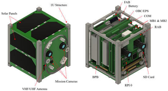
Figure 3.
BIRDS-5S system design.
Figure 4 illustrates the block diagram connections between OBC and the IMG-CLS Mission. The IMG-CLS mission hardware consists of commercial off-the-shelf (COTs) components due to their ease of availability and low cost. The primary components are a Raspberry Pi Zero (RPi0) microcontroller with the principal specifications described in Table 1, an Arducam OV5647 5MP Camera, and a SanDisk Industrial Grade 16Gb SD Card. The mission components for IMG-CLS were mounted onto the RAB of the satellite shown and connected to the OBC via SPI/UART and D-I/O connections to allow data communication, data transfer, and power control. The OBC manages the power supply and read/write access to onboard flash memory. The IMG-CLS mission captures and gives inferences on data to then organize and prioritize. The data are then written on the SD card and OBC flash memory, which can be accessed and downlinked to ground station operators. According to NASA guidelines for Raspberry Pis in space [23], it is considered necessary to test the SD cards before space flight. This SD card was chosen due to its robust performance in high temperature and vibration conditions. Radiation testing was conducted following guidelines to verify its performance in space conditions. The module was subjected to 200 Gy of radiation from a Co-60 radiation source over 6 h. The read/write capability of the SD card was verified during and after testing to ensure its in-space capability. Thermal Vacuum Testing (TVT) was also conducted to ensure the components can survive the temperature fluctuations and vacuum of space. To simulate the space environment, the satellite was subjected to a temperature range of −40 to +60 degrees Celsius in a vacuum at < Pa over multiple cycles. The mission was executed successfully under these conditions, and its capability in space was verified. Various satellite projects [24,25,26,27,28] have been launched using RPi as a primary or mission microcontroller, which validates its performance and viability for small-satellite implementations.
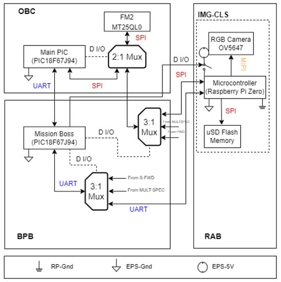
Figure 4.
Block diagram of the BIRDS-5S OBC and IMG-CLS missions.

Table 1.
Principal specifications of Raspberry Pi Zero.
2.2. Segmentation Dataset
This research focuses on the onboard prioritization of captured RGB images to provide ground station operators with remote-sensing data that would be viable for outreach purposes and further scientific research. With this in mind, the first step from Figure 5 involves using RGB images as inputs for the proposed algorithm. Manually collecting, segmenting, and labeling real-world nanosatellite data are tedious tasks that would hamper timely development. Therefore, a technique was developed to semi-automatically generate a large multi-class segmentation dataset. The dataset used as inputs for this algorithm was developed from images captured from the Sentinel-2 Earth Observation Satellite [29] at a Ground Sampling Distance (GSD) of 1000 m, 500 m, and 250 m. These data are meant to simulate captured images from nanosatellites with similar GSD parameters. Sentinel-2 data were used for this research as previous machine learning implementations [30,31,32,33] obtained viable results for nanosatellite implementations. Sentinel-2 provides a True Color Image (TCI) and a Scene Classification Map (SCL) constructed from multi-spectral data. The TCI product maps Sentinel-2 band values B04, B03, and B02, which roughly correspond to red, green, and blue parts of the spectrum, respectively, to R, G, and B components and form an RGB input image. The SCL product was developed by ESA to distinguish between cloudy pixels, clear pixels, and water pixels of Sentinel-2 data. The SCL map was reconstructed to combine classes to primarily represent 5 main classes of pixels in this research. These main classes are Water, Vegetation, Non-Vegetation, Cloud, and Unclassified. The SCL was used as the ground truth segmentation map, which clearly describes the scene features for the corresponding TCI product.
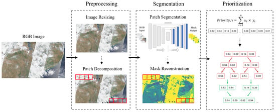
Figure 5.
Flowchart of the proposed algorithm.
An important step for improving the efficiency and performance of the algorithm is adjusting the input size of the image. This step can significantly improve the inference time for the selected segmentation architecture. For a single convolutional layer, the number of operations is directly proportional to the image size; thus, reducing image size will reduce the computational load for machine learning architectures. Furthermore, this step also ensures that an image of any input size can be used within the algorithm and produce a corresponding segmentation map. In addition to the computational benefits, the reduced input size also enables training on smaller images. This aspect simplifies the fine-tuning process after the nanosatellite is deployed in orbit, as more thumbnail images can be obtained for training compared to the original images. Despite the advantages in computational efficiency and training, it is important to acknowledge that reducing the input size compromises image resolution. Consequently, the accuracy of the segmentation class estimation by the Convolutional Neural Network (CNN) decreases, as the CNN faces challenges in learning from small features.
Patch decomposition is used as it is a valuable technique in machine learning, particularly in computer vision, where images often exhibit spatial locality. By breaking images down into smaller patches or sub-regions, this approach captures local patterns, supports translation invariance, and facilitates feature extraction. This process is expressed in Figure 5 as red boxes creating individual patches. It reduces computational complexity during convolutional operations for each patch, making it more efficient to train the neural network on high-resolution images. Patch decomposition is especially useful for handling varied object sizes, adapting to irregular shapes, and serving as part of data augmentation strategies. In tasks like semantic segmentation, it aids in pixel-wise predictions by allowing models to focus on local features. Patch decomposition enhances the ability to learn detailed information from images by analyzing them in a more localized and context-aware manner. Patch decomposition, while offering advantages in local feature extraction for machine learning tasks, comes with inherent disadvantages. One notable drawback is the potential loss of the global context, as the technique focuses on localized information, overlooking relationships and structures across the entire image. Additionally, the increased model complexity associated with managing overlapping patches or varying patch sizes can pose challenges in terms of design, training, and interpretation. Border effects may arise due to the under-representation of information near patch boundaries, as described in [18], leading to artifacts in model predictions. Computational overhead is another concern, as real-time processing and inference on multiple patches independently can impact inference times. The sensitivity of patch-based methods to hyper-parameter choices, such as patch size and stride, necessitates careful tuning.
The number of patches, , generated for an image with a size is given by Equation (1) for a patch size with a stride width and a stride height . Figure 6 illustrates the patch decomposition process implemented on the full-scale TCI and SCL products. The patch size was selected as as this factor would ensure that training features can capture local patterns while maintaining an acceptable resolution. Furthermore, the patch size was selected as a perfect square to reduce loss in the outermost boundaries of the patches due to a lack of information [30]. The stride was also selected as to ensure that the decomposition process perfectly tiles the entire image, leaving no gaps in between each patch. This technique generated a segmentation dataset containing 13,000 patch images and corresponding ground truth masks. These data were split into an 80:20 ratio of training data and test data for training the CNN architectures. In addition to this, data augmentation was conducted during dataset preparation to improve model performance and robustness. By introducing variations such as rotations, flips, and changes in brightness, the augmented dataset enhances the model’s generalization capabilities and mitigates overfitting risks.
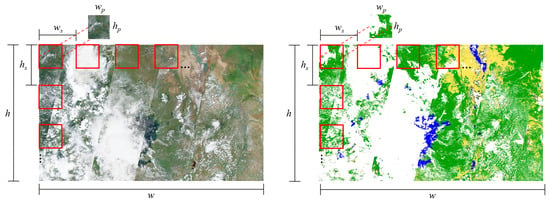
Figure 6.
Patch decomposition used for dataset creation.
2.3. Segmentation Architecture
The Convolutional Neural Network (CNN) was chosen as the primary technique for development. This technique was chosen due to its lightweight design and excellent performance in resource-limited applications. CNNs present several advantages that make them highly effective in various machine-learning tasks, particularly in the domain of computer vision. One key strength lies in their ability to automatically learn hierarchical representations of features from input data through convolutional layers, allowing them to discern patterns, textures, and spatial relationships in a data-driven manner. The shared weight architecture of CNNs significantly reduces the number of parameters compared to fully connected networks, enhancing computational efficiency and making them particularly suitable for large-scale datasets. Moreover, the local connectivity and weight sharing enable CNNs to capture translational invariance, making them robust to variations in the spatial location of features within an input. The hierarchical feature extraction, coupled with the use of pooling layers, allows CNNs to effectively abstract and represent complex structures in data, leading to their widespread success in image recognition, object detection, and other visual perception tasks. Overall, the adaptability, parameter efficiency, and ability to automatically learn hierarchical features contribute to the effectiveness of CNNs in handling complex visual information. Figure 7 shows four distinct design architectures that were considered for implementation, each chosen based on specific merits aligned with the research objectives.
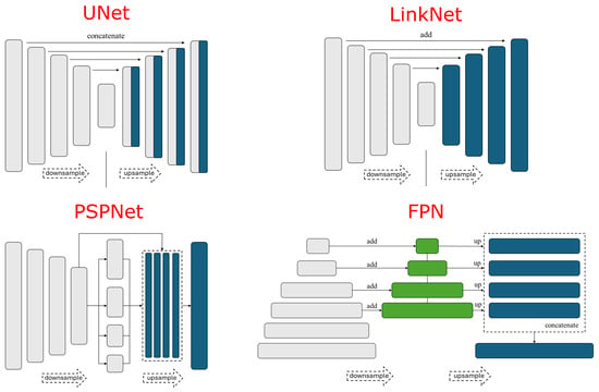
Figure 7.
Architecture designs for UNet, LinkNet, PSPNet and FPN.
UNet [20], was selected for its proven efficacy in semantic segmentation tasks. UNet’s unique encoder–decoder structure and skip connections facilitate the precise localization of objects in images, making it well suited for applications where spatial accuracy is paramount. From Table 2, UNet is effective for tasks needing precise object boundaries but has a large model size and complexity, leading to potential overfitting and higher memory usage.

Table 2.
Comparison of architecture designs.
LinkNet [15] was chosen for its emphasis on fast and efficient segmentation. LinkNet offers a faster inference speed and lower model size compared to UNet. This makes it a more lightweight option, suitable for applications where rapid processing is required. However, LinkNet may struggle with handling fine details due to its simpler design. It is also important to note that LinkNet is more suitable for tasks where speed is prioritized over detailed segmentation.
The Feature Pyramid Network (FPN) [34], the third architecture, was considered due to its proficiency in handling scale variations within images. FPN’s top-down architecture and lateral connections enable the network to capture multi-scale features effectively, addressing challenges associated with objects of varying sizes. FPN offers a balanced approach, with strong performance at different scales. Its Feature Pyramid architecture allows it to scale objects effectively, making it suitable for tasks where objects may vary in size or require multi-scale processing. However, FPN’s complexity and slower inference speed may be limiting factors in certain applications.
Lastly, the Pyramid Scene Parsing Network (PSPNet) [13] was selected for its prowess in capturing global context information. PSPNet utilizes pyramid pooling modules to aggregate contextual information at different scales, enhancing the model’s ability to understand complex scene structures. PSPNet excels in capturing global context, making it a strong choice for tasks requiring a high level of contextual information. Its ability to capture long-range dependencies can lead to improved accuracy in semantic segmentation. However, PSPNet’s higher complexity and memory consumption may limit its applicability in resource-constrained environments or in real-time applications where speed is crucial. The comprehensive consideration of these diverse architectures reflects a strategic approach to evaluating segmentation models, aiming to leverage their respective strengths for optimal performance in the specific context of the research.
Furthermore, various backbone designs were used in conjunction with the listed architectures. Some of these backbone designs include ResNet34, SEResNeXt50, MobileNetV2, and EfficientNetB0. These backbone architectures were chosen to leverage high-performance capability while also managing training time, inference time, model parameter size, and TFLite model size. The choice of ResNet34 as a backbone design is motivated by its strong representation learning capabilities. ResNet architectures, with skip connections and residual blocks, facilitate the training of deep networks, enabling effective feature extraction. However, ResNet34’s main disadvantage is its relatively larger model size and higher computational demands compared to lighter architectures like MobileNetV2 and EfficientNetB0.
SEResNeXt50, on the other hand, was chosen for its enhanced efficiency in learning diverse features. The combination of Squeeze and Excitation (SE) blocks with a powerful ResNeXt backbone enhances feature recalibration, contributing to its improved segmentation performance. However, SEResNeXt50’s main disadvantage is its higher computational complexity compared to simpler architectures like MobileNetV2.
In scenarios where computational resources are constrained, MobileNetV2 is a valuable choice due to its lightweight architecture. MobileNetV2 strikes a balance between model efficiency and performance, making it suitable for applications with limited resources. However, MobileNetV2 may struggle with capturing fine details compared to deeper architectures like ResNet34 and SEResNeXt50.
EfficientNetB0, known for its optimal scaling of model depth, width, and resolution, offers a scalable solution to adapt to various computational constraints. It provides a good balance between model size and performance, making it suitable for a wide range of applications. However, EfficientNetB0 may require more training data compared to other architectures to achieve optimal performance.
The strategic integration of these backbone designs with the segmentation architectures aims to exploit their specific advantages, ensuring an optimal trade-off between model complexity and performance across different aspects crucial for the successful deployment of the models in resource-constrained environments.
2.4. Evaluation Metrics
Segmentation algorithms are evaluated using various metrics to assess their performance in accurately delineating objects or regions of interest within images. The Intersection over Union () or Jaccard Index measures the overlap between the predicted segmentation and the ground truth. It is computed as the intersection of the predicted and true segmentations divided by their union. is a widely used metric for assessing the spatial accuracy of segmentations. The formula for is given by the intersection of the predicted and true segmentations divided by their union, as shown in Equation (2):
The Mean IoU () extends this metric to multiple classes, providing an average IoU value across all classes. The formula for is
where N is the number of classes, and is the for class i. The is a valuable metric as it considers the performance across different classes, providing a more comprehensive assessment of the segmentation algorithm’s accuracy. A higher indicates better overall segmentation performance, with larger values signifying improved spatial alignment between predicted and true segmentations across diverse classes. This metric is particularly useful in scenarios where the segmentation task involves recognizing and delineating multiple distinct categories or objects within an image. , , and are commonly used metrics for evaluating the performance of classification and segmentation algorithms. They provide insights into different aspects of model accuracy, particularly in tasks where the trade-off between false positives and false negatives is crucial. measures the accuracy of positive predictions, indicating the fraction of predicted positive instances that are correctly classified. It is computed as the ratio of true positives to the sum of true positives and false positives. quantifies the ability of the model to capture all relevant instances of a particular class. It is calculated as the ratio of true positives to the sum of true positives and false negatives.
The is the harmonic mean of precision and recall. It provides a balanced measure that considers both false positives and false negatives. The reaches its maximum value of 1 when precision and recall are both perfect.
In addition to this, we use the percentage coverage estimate for each class, which is given by the equation:
where
- is the coverage for class c in the image;
- represents the pixel value for class c at position in the image;
- a is the width of the image;
- b is the height of the image.
The evaluation metrics are important for assessing class coverage accuracy as they provide a quantitative measure of how well the segmentation algorithm is performing. A high precision value indicates that the model’s positive predictions are likely to be accurate, while a high recall value signifies the model’s ability to capture a substantial portion of true positive instances. Mean IoU evaluates the spatial alignment between predicted and true segmentations, indicating the accuracy of the segmentation results. The , , and assess the algorithm’s ability to correctly classify pixels into different classes, providing insights into the model’s overall performance. By considering these metrics, we can prioritize class coverage based on the quality of segmentation, ensuring that images with more accurate and reliable class delineation are given higher priority for downlinking. This approach helps improve the overall quality of the downlinked data, leading to more meaningful and reliable remote sensing observations.
The choice of weightings for each class is based on the significance of the class in the context of remote sensing applications. The “Unclassified” class is given a weighting of 0 because we do not want to downlink images with unclassified data, as they do not provide meaningful information for analysis. The “Cloud” class is given a weighting of 1 because while it is important to avoid downlinking cloudy images, it is also expected that all images will contain some level of cloud cover. Therefore, images will be prioritized based on the percentage of cloud cover, with less cloudy images being given higher priority. The Vegetation, Non-vegetation, and Water classes are given a weighting of 2 because they are typically of high interest in remote sensing applications. Vegetation, for example, is important for monitoring vegetation health and land cover change, while water bodies are critical for water resource management and environmental monitoring. Prioritizing the downlinking of images with these classes can provide valuable insights into environmental conditions and ecosystem health. By using these weightings in the prioritization equation, we can ensure that images with more meaningful and relevant content are given higher priority for downlinking, leading to more efficient use of limited downlink resources and better utilization of satellite data for remote sensing applications.
where
- is the weighting assigned to class c;
- n is the number of classes;
- is the priority index.
Finally, the images are prioritized based on the priority index of each image. The Timsort algorithm is used in this study for the ranking of the images for downlink prioritization. Timsort is a hybrid sorting algorithm derived from merge sort and insertion sort, designed to provide both efficiency and adaptability to various data structures and sizes.
3. Results
This section describes the results obtained from the training and testing of the image prioritization algorithm. The models were built using Keras 2.9.0 and Tensorflow 2.9.1 using Python 3.9. The models were trained using an NVIDIA RTX 3070 Ti sourced from Kitakyushu, Japan.
3.1. Model Performance Testing
From the assortment of architectures and backbone designs detailed in Section 2.3, multiple combinations were trained and evaluated to assess their efficacy for the segmentation task. Figure 8 illustrates the performance of different model architectures on the testing dataset.
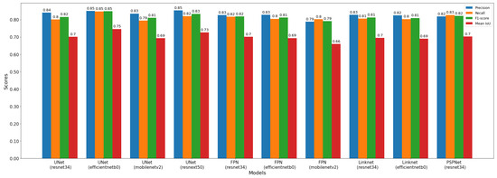
Figure 8.
Comparison of model performances.
The top-performing model among those examined is the Unet with an EfficientNetB0 backbone, achieving the highest Mean IoU of 0.75, F1 Score of 0.85, and recall and precision scores of 0.85. This suggests that leveraging the EfficientNetB0 backbone enhances the model’s ability to accurately segment objects in the images. Conversely, the least effective model appears to be FPN with a MobileNetV2 backbone, attaining the lowest mean of 0.66 and of 0.79, along with relatively lower recall and precision scores compared to other models. This implies that the MobileNetV2 backbone may not adequately capture the necessary features for segmentation.
Notable differences in performance are observed when changing backbones across models. While Unet and FPN with a ResNet34 backbone exhibit comparable Mean IoU and , they outperform LinkNet with the same backbone, indicating the influence of architecture variations on model performance, even with identical backbones. Moreover, Unet consistently outperforms other architectures across different backbones, highlighting its robustness for the segmentation task.
In terms of computational efficiency, models with lighter backbones such as MobileNetV2 and EfficientNetB0 generally demonstrate lower performance compared to those with heavier backbones like ResNet34 and SEResNeXt50. However, this efficiency comes at the expense of slightly lower segmentation accuracy.
It is worth noting that the highest-performing architecture was Unet (EfficientNetB0). This could be attributed to faster training convergence for this model, possibly influenced by the small dataset size. Similarly, comparing different architectures with the same backbone, such as Unet, FPN, LinkNet, and PSPNet with a ResNet34 backbone, reveals slight variations in performance metrics but generally similar trends. The findings underscore the critical role of backbone choice and architecture selection in achieving optimal performance for the segmentation task.
In Figure 9, the ground truth coverage versus the predicted coverage is depicted for the four top-performing models with varying architectures. Across all models, the segmentation and classification of the test data into specific classes are executed excellently, albeit with minor outliers observed in certain cases, particularly in the classification of water and clouds. However, such occurrences are minimal across the four tested models. The coefficient of determination, , calculated for each plot, signifies the models’ capability to predict the classes of the observed data with high accuracy. Notably, the UNet model achieves the highest value of 0.97, which correlates with its excellent Mean IoU performance of 0.75. Additionally, the standard deviation illustrates tightly clustered prediction performance, indicating high accuracy and precision. Although LinkNet and FPN achieved similar Mean IoU values, their values of 0.93 and 0.95, respectively, were slightly lower than those of UNet. Moreover, their standard deviations, especially for LinkNet, are slightly larger, suggesting less precise predictions. PSPNet achieved an value of 0.95 on the test dataset, with similar accuracy and precision spread to UNet, affirming its viability for segmentation implementation.
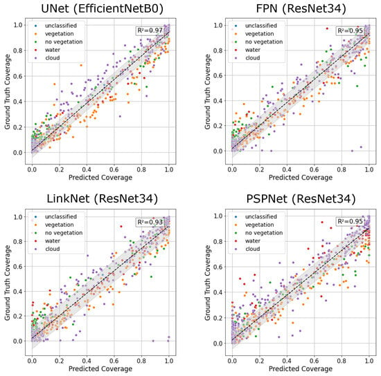
Figure 9.
The ground truth class coverage of the test dataset plotted against the predicted class coverage.
Figure 10 presents a visual comparison of the different models’ performance on a separate validation dataset sourced from the Sentinel satellite. The true color (RGB) images and associated coverage masks are illustrated in the figure in the first two columns. The predictions of the four best-performing models are also illustrated in the figure to compare against the ground truth coverage. Overall, the models demonstrate excellent performance in segmenting and classifying image components compared to ground truth. Notably, prominent features such as clouds and water bodies are segmented accurately. However, challenges arise in accurately segmenting water bodies in intensely brown areas, such as flooded regions, where models may struggle. Additionally, deep dark features, especially in the center of water bodies, occasionally lead to misidentification as unclassified areas. While UNet and FPN perform well across all validation images, they encounter difficulties in accurately distinguishing dark water bodies from unclassified regions in some cases. LinkNet excels in detecting dark water bodies but may occasionally misclassify cloudy areas. Conversely, PSPNet consistently exhibits excellent performance across all image areas, corroborating its high Mean IoU and performance metrics.
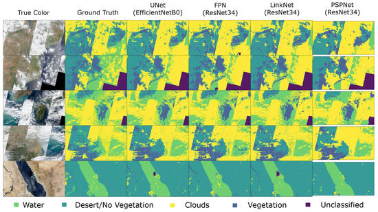
Figure 10.
A visual comparison of the ground truth coverage and model coverage prediction performances.
Table 3 illustrates the evaluation of varying the patch sizes for training and inference execution for the UNet (EfficientNetB0) model. As the patch size decreases, the training time tends to increase. This is because smaller patch sizes result in more patches to process, leading to a longer training duration. For both image sizes, the training time increases as the patch size decreases from 64 × 64 to 16 × 16. The single patch inference time remains relatively stable across different patch sizes for both image sizes. The full image inference time, which is the time required to process the entire image during inference, increases significantly as the patch size decreases. This is expected since smaller patch sizes result in more patches, leading to a longer overall inference time. For example, for the 640 × 480 image size, the full image inference time increases from 8.4 s for a 64 × 64 patch size to 137.5 s for a 16 × 16 patch size. The metric shows no clear correlation between patch size and . However, it is worth noting that there is a slight decrease in as the patch size decreases, particularly for the 16 × 16 patch size.

Table 3.
Evaluation of patch size selection.
3.2. Hardware Performance Testing
For each model architecture and backbone design outlined in Table 4, corresponding training parameters, training times, file sizes, and inference execution times were evaluated. The inference execution times were assessed on both the RPi0 and the RPi4 to compare computation performance across different hardware setups. The overall model parameters for each design are influenced by the chosen architecture and backbone. MobileNetV2 and EfficientNetB0 were selected as backbone candidates due to their low parameter count, leading to shorter training times and smaller model file sizes. Consistently, these backbone designs exhibit lower parameter counts, training times, and model file sizes, resulting in faster inference execution times on the implementation hardware.

Table 4.
Model characteristics.
Conversely, the UNet (SEResNext50) design has the highest parameter count, training time, file size, and execution time among all designs. This is expected due to its deeper network architecture and implementation of Squeeze and Excitation (SE) blocks, which enhance performance at the expense of computational demands. In some instances, the RPi0 faced resource exhaustion during inference execution, highlighting the delicate balance between managing parameter count and performance.
Across all model sizes, loading the TensorFlow library on the RPi0 consistently emerged as the most time-consuming step, contributing to increased inference execution times. PSPNet (ResNet34) features a notably low parameter count due to adjustments in the input size while maintaining high accuracy and inference execution time on both hardware setups. Ultimately, UNet (EfficientNetB0) emerged as the best-performing model in terms of tradeoffs between computational load and inference performance.
Figure 11 illustrates the hardware performance testing for both satellite hardware test devices. The hardware is tasked with executing inference using the UNet (EfficientNetB0) model on a 1250 × 760 image, which equates to 209 patches of size . As expected, the RPi4 demonstrates superior model execution performance owing to its greater computational resources compared to the RPi0. During inference, the RPi4 experiences a significant increase in CPU temperature from 50.5 °C to a peak of 58.0 °C, while the RPi0 maintains a relatively stable temperature of around 43.5 °C throughout the sequence. This highlights the robust computational capabilities of the RPi4, albeit with considerations for thermal management, particularly in space operations.
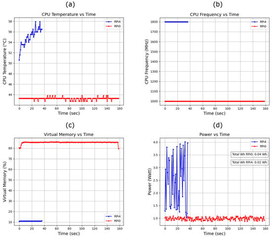
Figure 11.
Hardware performance testing comparing (a) CPU temperature, (b) CPU frequency, (c) virtual memory, (d) power consumption.
The RPi0 operates at 85% virtual memory utilization and sustains a 100% CPU Frequency load at 1 GHz, while the RPi4 utilizes only 10% of memory at 1.8 GHz. In terms of power consumption over execution time, the RPi0 shows a peak consumption of around 1 W, with a total energy consumption of 0.04 Wh. In comparison, the RPi4 exhibits fluctuating power consumption, attributed to power and temperature management software features, with a peak load of 4.1 W and a total consumption of 0.2 Wh. This underscores the lower sustained load of the RPi0 but demands a higher power budget for longer execution times, particularly in space operations.
3.3. Validation Testing
To evaluate the performance of the prioritization algorithm, we use data from the BIRDS-4 Nanosatellite [21]. This dataset comprises images downlinked throughout the BIRDS-4 satellite’s lifespan, serving as a reliable representation of the expected downlink data budget for the BIRDS-5S satellite. Organized and manually segmented, this dataset forms a validation dataset for testing the algorithm’s efficacy.
The dataset encompasses images suitable for remote sensing or outreach, characterized by nadir-pointing Earth-facing perspectives with minimal cloud coverage. However, it also includes images captured while the satellite is tumbling in orbit, resulting in unfocused Earth images, as well as images with high cloud cover or solely capturing space, rendering them unsuitable for research or outreach purposes.
For inference execution and coverage estimation, we utilize the UNet (EfficientNetB0) model, which was selected for its exceptional segmentation performance while managing computational load effectively on the target hardware. Figure 12 visually illustrates the segmentation performance of the model on the test dataset, demonstrating its excellence in handling unseen data. The predicted segmentation coverage closely aligns with the ground truth mask in all cases, affirming the model’s adaptability to diverse input images from different hardware designs.
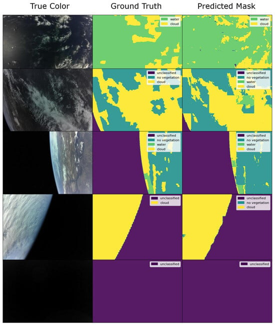
Figure 12.
A visual illustration of the validation dataset test performance.
Furthermore, Figure 13a showcases the ground truth priority versus the predicted priority for the dataset images. The value, calculated at 0.96, signifies excellent performance and tight precision, as indicated by the associated standard deviation depicted in the shaded region. The estimated predictions based on coverage maps closely match the ground truth, underscoring the model’s segmentation accuracy and subsequent priority assignment capabilities. This plot also describes the distribution of data within the validation dataset. From analysis, we can see that a large number of images are classified with low or 0 priority in the graph. This indicates that these images are primarily captures of space or very cloudy regions. The algorithm accurately predicts the coverage map and priority for these images; however, in some cases, it has difficulty due to features such as sunlight saturation in some validation images.
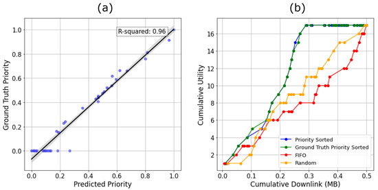
Figure 13.
Prioritization performance showing (a) ground truth priority and predicted priority. (b) Cumulative Utility and cumulative downlink for four scheduling methods, showing that Priority Sorted achieves the highest utility.
To evaluate the prioritization algorithm’s performance for downlink efficiency, we can use the Cumulative Utility metric described by Doran [33] for image prioritization. Each image in the dataset is assigned a utility value of 1 if deemed useful for remote sensing or outreach and 0 otherwise. Figure 13b illustrates the Cumulative Utility against the Cumulative Downlink data budget. Each plot represents the downlink of data based on a prioritization method. Priority and ground truth priority sorting describe the downlink of data that is sorted according to priority indexes calculated from the coverage and ground truth predictions, respectively. FIFO represents the downlink of data in chronological order as downlinked by the BIRDS-4 satellite during its lifetime.
Notably, the priority-sorted algorithm achieves maximum utility at 0.29MB, compared to the FIFO downlink, which reaches maximum utility at 0.5MB, representing a 42% improvement in data budget efficiency. These results highlight the prioritization algorithm’s efficacy in optimizing downlink efficiency while maintaining alignment with ground truth priorities, underscoring its potential for real-world deployment in satellite operations. This efficiency gain is particularly valuable in scenarios where downlink opportunities are limited, such as during short satellite passes or when constellation satellites are competing for downlink resources. By optimizing downlink efficiency, the algorithm ensures that critical data are prioritized for transmission, maximizing the overall value and impact of satellite missions. The randomly sorted priority downlink is also plotted and illustrated. The predicted priority sorting and ground truth sorting match almost perfectly, and both algorithms achieve maximum utility with the same cumulative downlink, which indicates the model performs almost perfectly on the test dataset. Random sorting also shows the deviation between the FIFO sorting and priority sorting. We can see that the FIFO method is the least efficient when compared to all methods, which indicates the potential usefulness of the proposed onboard prioritization and sorting algorithm.
To illustrate the performance of the designed algorithm and its applicability for multiple classes of nanosatellites, we compare the power consumption efficiency and the utility achieved when using this prioritization solution. Figure 14 shows the Cumulative Utility vs. the cumulative power consumption for a 1 U and 6 U class nanosatellite. The BIRDS-5S 1 U nanosatellite operates using VHF/UHF communication systems. The 6U satellite data used for this testing are based on the KITSUNE 6 U nanosatellite [28], which has a C-band communication array. Using test data for the C-band downlink and RPi CM4 processing, we see that the 6 U satellite consumes approximately 7.40 Wh to downlink the full validation test dataset without priority processing and discarding of images. The 1 U satellite consumes 12.15 Wh to downlink the full validation test set using VHF/UHF communication systems. Even though the operating power required to downlink data using the UHF/VHF transceiver is lower, the operating time is significantly longer as the data rate is slower, which leads to the 1 U satellite consuming more power to downlink the same data. When the prioritization algorithm is used, the processing of each image consumes approximately 0.02 Wh for the 1 U satellite using an RPi0. However, the algorithm selects which images to discard and thus reduces the data budget and subsequent downlink time. The operating time of the VHF/UHF transceiver is reduced, and the dataset can be downlinked, consuming approximately 7.73 Wh.
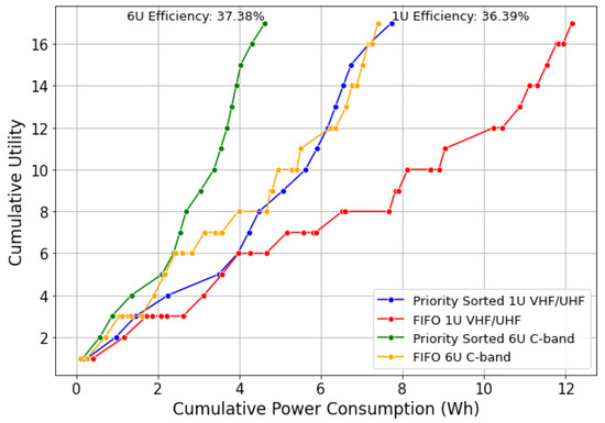
Figure 14.
Prioritization performance, which illustrates Cumulative Utility vs. cumulative power consumption for a 1U satellite with UHF/VHF communication and a 6U with C-band communication systems.
This reduction in power consumption of the 1 U satellite indicates a power efficiency of 36.39% when using the priority sorting algorithm. For the 6 U satellite, the processing of each image consumes 0.04 Wh, but reducing the operating time for the C-band also reduces the total consumed power. When using the priority sorting algorithm, the 6 U can achieve a downlink of data with a 37.38% power efficiency. These results suggest that the prioritization algorithm can become a standard onboard implementation in future satellite missions, enhancing overall mission performance and resource utilization. A variant of this research is currently under implementation for the upcoming VERTECS 6 U nanosatellite [35], which carries a Raspberry Pi Compute Module 4 as the primary microcontroller for the Camera Controller Board (CCB).
The Kyutech GS typically achieves a downlink speed of 4800–9600 bps using the VHF-UHF downlink frequency range. With this, operators can typically initiate a downlink of approximately 150 packets of data, with each packet containing 81 bytes. Satellites in the LEO orbit revisit approximately three times per day, with approximately 75% of a pass being usable for downlink. Using these data, we can infer an estimated 1 day of operation to downlink one thumbnail operation, 2–3 days for 1 VGA image, and 3–5 days for a 1280 × 960 image. Therefore, we can see that a priority sorting data algorithm and achieving high downlink utility can save operators a significant amount of time and therefore improve downlink efficiency.
In this validation test, 0.21 MB of data can be ignored as they were deemed useless for outreach/science purposes, which represents an estimated 98 days of downlink operations. When considering the power consumption efficiency estimates from the previous analysis, which showed a 36.39% improvement for the 1 U satellite and a 37.38% improvement for the 6 U satellite when using the prioritization algorithm, the combined benefits of reduced power consumption and improved downlink efficiency demonstrate the viability and practical applications of this research for nanosatellites conducting remote sensing and outreach operations.
To fully assess the capacity of this research to improve the remote sensing applications of nanosatellites, a visual comparison of performance for cloud coverage estimation and prioritization was also conducted. Cloud cover is detrimental to remote sensing data because it obscures the view of the Earth’s surface, reducing the amount of usable data that can be captured and affecting the quality and accuracy of the imagery.
Figure 15 illustrates the True Color image captured from the Sentinal-2 satellite at a GSD of 60 m and the ground truth cloud coverage map. The scene represents the same target location captured at different cloud coverage percentages. To compare the performance of this research, we selected the network architectures proposed by Jeppesen [18] and Zhang [19] due to their robustness and extensive validation in the field of remote sensing. These architectures have been widely adopted and rigorously evaluated, serving as strong benchmarks for assessing the efficacy and novelty of our proposed approach.
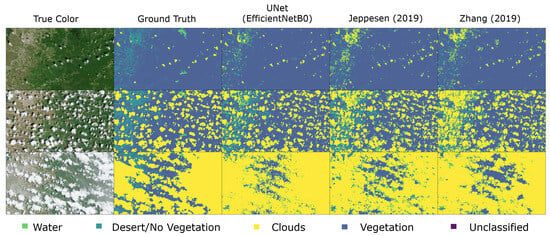
Figure 15.
A visual comparison of the performance of UNet (EfficientNetB0), Jeppesen [18] and Zhang [19].
From the results, we can see that all three networks perform excellently in segmenting the cloud coverage map. For low cloud coverage, UNet (EfficientNetB0) achieves a of 93.4% for cloud cover estimation and 74.3% for multi-class scene classification. Jeppesen and Zhang achieved 91.7% and 90.3% for cloud cover assessment. For multi-class scene classification, the architectures achieve 73.2% and 74.0%, respectively. Jeppesen and Zhang both utilize UNet-based architectures, so the performance is similar to the proposed algorithm. However, the proposed algorithm applies deeper layers using the EfficientNetB0 backbone as the encoder step for feature extraction. These deeper layers translate to more improved performance in multi-class segmentation.
For medium cloud coverage, the three models achieve similar results with a cloud coverage estimation of 91.1%, 90.7%, and 90.3%, respectively. For multi-classification, they achieve 74.2%, 72.7%, and 72.2%, respectively. These results illustrate the ability of the algorithms to accurately gauge cloud cover at varying levels. For high cloud cover with varying types of clouds, such as cirrus, the three models exhibit slight variations in performance. The UNet (EfficientNetB0) model continues to demonstrate its effectiveness, achieving a cloud coverage estimation of 87.5%. In comparison, the Jeppesen model achieves 87.8%, and the Zhang model achieves 87.3%. These results indicate that even at high cloud cover with varying types of clouds, the proposed method is capable of achieving comparable performance to dedicated cloud cover assessment solutions.
This performance consistency across different cloud types underscores the proposed solution’s robustness and adaptability. The accurate segmentation of the data produces quantifiable prioritization metrics using the proposed algorithm. In this test, these prioritization values are used to discard the high cloud cover data and prioritize the low cloud cover data with coverage assessments of the vegetation and non-vegetative components. These results illustrate the proposed algorithm’s use as a valuable tool for onboard remote sensing applications requiring accurate cloud cover and scene assessment.
4. Conclusions
The culmination of this investigation into model performance testing, hardware capabilities, and validation testing outcomes reveals a promising outlook for the application of the prioritization algorithm in satellite operations. Through an analysis of various model architectures and backbone designs, we have assessed various performance characteristics of existing model designs and illustrated the trade-off between segmentation performance and model design. The UNet (EfficientNetB0) model illustrates excellent segmentation accuracy with a Mean IoU of 0.75 and an F1 Score of 0.85 while efficiently managing computational resources. Moreover, hardware performance testing has shed light on the computational capabilities and management considerations of satellite hardware setups, emphasizing the need for a balanced approach to computational efficiency and power constraints.
In validation testing, the prioritization algorithm has demonstrated its effectiveness in optimizing downlink efficiency while remaining aligned with ground truth priorities, showcasing robust segmentation accuracy with an value of 0.96 and adaptability to diverse image inputs. The algorithm also achieves a 42% improvement in data budget efficiency and an estimated 36.39% power efficiency based on validation testing, highlighting its efficacy in optimizing downlink and satellite operations. Additionally, the analysis of cloud cover assessment using the algorithm has shown its ability to accurately gauge cloud cover, further enhancing its utility in satellite operations.
These findings collectively show the potential of the prioritization algorithm to enhance data utilization and decision-making in satellite missions to prepare for its deployment in real-world scenarios. The BIRDS-5S Satellite is scheduled to launch in early 2025, and the findings of this research are expected to inform its operations, showcasing the practical impact of this study on real-world satellite missions.
Supplementary Materials
The following supporting information can be downloaded at https://www.mdpi.com/article/10.3390/rs16101729/s1.
Author Contributions
Conceptualization, K.C., K.K. and M.C.; methodology, K.C., K.K. and M.C.; software, K.C.; validation, K.C., K.K. and M.C.; formal analysis, K.C., K.K. and M.C.; investigation, K.C., K.K. and M.C.; resources, K.C., K.K. and M.C.; data curation, K.C. and M.C.; writing—original draft preparation, K.C.; writing—review and editing, K.C., K.K. and M.C.; visualization, K.C.; supervision, K.K. and M.C.; project administration, K.K. and M.C.; funding acquisition, K.K. and M.C. All authors have read and agreed to the published version of the manuscript.
Funding
This research received no external funding.
Data Availability Statement
The following are available in the Supplementary Material. The Training, Test, and Validation Datasets contain images and masks of size and , respectively. The original contributions presented in the study are included in the article and Supplementary Material, further inquiries can be directed to the corresponding author.
Acknowledgments
The authors would like to express appreciation for the valuable comments of the associated editors and anonymous reviewers.
Conflicts of Interest
The authors declare no conflicts of interest.
Abbreviations
The following abbreviations are used in this manuscript:
| CNN | Convolutional Neural Network |
| mIoU | Mean Intersection of Union |
| CubeSat | Nanosatellite |
| HF | High Frequency |
| UHF | Ultra High Frequency |
| GMSK | Gaussian minimum-shift keying |
| BPSK | Binary Phase-Shift Keying |
| FSK | Frequency-shift keying |
| AFSK | Audio frequency-shift keying |
| GFSK | Gaussian Frequency-shift keying |
| PSPNet | Pyramid Spatial Pooling Network |
| CSI | Critical Success Index |
| CS-CNN | Cloud Segmentation Convolutional Neural Network |
| OBC | Onboard Computer |
| EPS | Electrical Power System |
| COM | Communication System |
| RAB | Rear Access Board |
| BPB | Backplane Board |
| MULT-SPEC | Multispectral Imaging mission |
| S-FWD/APRS | Store-and-Forward/Digital Repeating mission |
| IMG-CLS | Image Classification mission |
| CPLD | Complex Programmable Logic Device |
| RPi0 | Raspberry Pi Zero |
| TVT | Thermal Vaccum Testing |
| GSD | Ground Sampling Distance |
| TCI | True Color Image |
| SCL | Scene Classification Map |
| FPN | Feature Pyramid Network |
References
- Heidt, H.; Puig-Suari, J.; Moore, A.S.; Nakasuka, S.; Twiggs, R.J. CubeSat: A new Generation of Picosatellite for Education and Industry Low-Cost Space Experimentation. In Proceedings of the AIAA/USU Conference on Small Satellites, Logan, UT, USA, 6–11 August 2000. [Google Scholar]
- Francisco, C.; Henriques, R.; Barbosa, S. A Review on CubeSat Missions for Ionospheric Science. Aerospace 2023, 10, 622. [Google Scholar] [CrossRef]
- Liu, S.; Theoharis, P.I.; Raad, R.; Tubbal, F.; Theoharis, A.; Iranmanesh, S.; Abulgasem, S.; Khan, M.U.A.; Matekovits, L. A survey on CubeSat missions and their antenna designs. Electronics 2022, 11, 2021. [Google Scholar] [CrossRef]
- Robson, D.J.; Cappelletti, C. Biomedical payloads: A maturing application for CubeSats. Acta Astronaut. 2022, 191, 394–403. [Google Scholar] [CrossRef]
- Bomani, B.M. CubeSat Technology Past and Present: Current State-of-the-Art Survey; Technical report; NASA: Washington, DC, USA, 2021. [Google Scholar]
- White, D.J.; Giannelos, I.; Zissimatos, A.; Kosmas, E.; Papadeas, D.; Papadeas, P.; Papamathaiou, M.; Roussos, N.; Tsiligiannis, V.; Charitopoulos, I. SatNOGS: Satellite Networked Open Ground Station; Valparaiso University: Valparaiso, IN, USA, 2015. [Google Scholar]
- Bouwmeester, J.; Guo, J. Survey of worldwide pico-and nanosatellite missions, distributions and subsystem technology. Acta Astronaut. 2010, 67, 854–862. [Google Scholar] [CrossRef]
- Nagel, G.W.; Novo, E.M.L.d.M.; Kampel, M. Nanosatellites applied to optical Earth observation: A review. Rev. Ambiente Água 2020, 15, e2513. [Google Scholar] [CrossRef]
- Eapen, A.M.; Bendoukha, S.A.; Al-Ali, R.; Sulaiman, A. A 6U CubeSat Platform for Low Earth Remote Sensing: DEWASAT-2 Mission Concept and Analysis. Aerospace 2023, 10, 815. [Google Scholar] [CrossRef]
- Zhao, M.; O’Loughlin, F. Mapping Irish Water Bodies: Comparison of Platforms, Indices and Water Body Type. Remote Sens. 2023, 15, 3677. [Google Scholar] [CrossRef]
- Rastinasab, V.; Hu, W.; Shahzad, W.; Abbas, S.M. CubeSat-Based Observations of Lunar Ice Water Using a 183 GHz Horn Antenna: Design and Optimization. Appl. Sci. 2023, 13, 9364. [Google Scholar] [CrossRef]
- Yuan, W.; Wang, J.; Xu, W. Shift pooling PSPNet: Rethinking pspnet for building extraction in remote sensing images from entire local feature pooling. Remote Sens. 2022, 14, 4889. [Google Scholar] [CrossRef]
- Zhao, H.; Shi, J.; Qi, X.; Wang, X.; Jia, J. Pyramid scene parsing network. In Proceedings of the IEEE Conference on Computer Vision and Pattern Recognition, Honolulu, HI, USA, 21–26 July 2017; pp. 2881–2890. [Google Scholar]
- Guo, X.; Wan, J.; Liu, S.; Xu, M.; Sheng, H.; Yasir, M. A scse-linknet deep learning model for daytime sea fog detection. Remote Sens. 2021, 13, 5163. [Google Scholar] [CrossRef]
- Chaurasia, A.; Culurciello, E. Linknet: Exploiting encoder representations for efficient semantic segmentation. In Proceedings of the 2017 IEEE Visual Communications and Image Processing (VCIP), St. Petersburg, FL, USA, 10–13 December 2017; pp. 1–4. [Google Scholar]
- King, M.D.; Platnick, S.; Menzel, W.P.; Ackerman, S.A.; Hubanks, P.A. Spatial and temporal distribution of clouds observed by MODIS onboard the Terra and Aqua satellites. IEEE Trans. Geosci. Remote Sens. 2013, 51, 3826–3852. [Google Scholar] [CrossRef]
- Drönner, J.; Korfhage, N.; Egli, S.; Mühling, M.; Thies, B.; Bendix, J.; Freisleben, B.; Seeger, B. Fast cloud segmentation using convolutional neural networks. Remote Sens. 2018, 10, 1782. [Google Scholar] [CrossRef]
- Jeppesen, J.H.; Jacobsen, R.H.; Inceoglu, F.; Toftegaard, T.S. A cloud detection algorithm for satellite imagery based on deep learning. Remote Sens. Environ. 2019, 229, 247–259. [Google Scholar] [CrossRef]
- Zhang, Z.; Iwasaki, A.; Xu, G.; Song, J. Cloud detection on small satellites based on lightweight U-net and image compression. J. Appl. Remote Sens. 2019, 13, 026502. [Google Scholar] [CrossRef]
- Ronneberger, O.; Fischer, P.; Brox, T. U-net: Convolutional networks for biomedical image segmentation. In Proceedings of the Medical Image Computing and Computer-Assisted Intervention–MICCAI 2015: 18th International Conference, Munich, Germany, 5–9 October 2015; Proceedings, Part III 18. pp. 234–241. [Google Scholar]
- Cespedes, A.J.J.; Bautista, I.Z.C.; Maeda, G.; Kim, S.; Masui, H.; Yamauchi, T.; Cho, M. An Overview of the BIRDS-4 Satellite Project and the First Satellite of Paraguay. In Proceedings of the 11th Nanosatellite Symposium, Online, 17 March 2021. [Google Scholar]
- Maskey, A.; Lepcha, P.; Shrestha, H.R.; Chamika, W.D.; Malmadayalage, T.L.D.; Kishimoto, M.; Kakimoto, Y.; Sasaki, Y.; Tumenjargal, T.; Maeda, G.; et al. One Year On-Orbit Results of Improved Bus, LoRa Demonstration and Novel Backplane Mission of a 1U CubeSat Constellation. Trans. Jpn. Soc. Aeronaut. Space Sci. 2022, 65, 213–220. [Google Scholar] [CrossRef]
- Guertin, S.M. Raspberry Pis for Space Guideline; NASA: Washington, DC, USA, 2022. [Google Scholar]
- Bai, X.; Oppel, P.; Cairns, I.H.; Eun, Y.; Monger, A.; Betters, C.; Musulin, Q.; Bowden-Reid, R.; Ho-Baillie, A.; Stals, T.; et al. The CUAVA-2 CubeSat: A Second Attempt to Fly the Remote Sensing, Space Weather Study and Earth Observation Instruments. In Proceedings of the 36th Annual Small Satellite Conference, Logan, UT, USA, 5–10 August 2023. [Google Scholar]
- Danos, J.; Page, C.; Jones, S.; Lewis, B. USU’s GASPACS CubeSat; USU: Logan, UT, USA, 2022. [Google Scholar]
- Garrido, C.; Obreque, E.; Vidal-Valladares, M.; Gutierrez, S.; Diaz Quezada, M.; Gonzalez, C.; Rojas, C.; Gutierrez, T. The First Chilean Satellite Swarm: Approach and Lessons Learned. In Proceedings of the 36th Annual Small Satellite Conference, Logan, UT, USA, 5–10 August 2023. [Google Scholar]
- Drzadinski, N.; Booth, S.; LaFuente, B.; Raible, D. Space Networking Implementation for Lunar Operations. In Proceedings of the 37th Annual Small Satellite Conference, Logan, UT, USA, 5–10 August 2023. number SSC23-IX-08. [Google Scholar]
- Azami, M.H.b.; Orger, N.C.; Schulz, V.H.; Oshiro, T.; Cho, M. Earth observation mission of a 6U CubeSat with a 5-meter resolution for wildfire image classification using convolution neural network approach. Remote Sens. 2022, 14, 1874. [Google Scholar] [CrossRef]
- Louis, J.; Debaecker, V.; Pflug, B.; Main-Knorn, M.; Bieniarz, J.; Mueller-Wilm, U.; Cadau, E.; Gascon, F. Sentinel-2 Sen2Cor: L2A processor for users. In Proceedings of the living planet symposium 2016, Prague, Czech Republic, 9–13 May 2016; pp. 1–8. [Google Scholar]
- Park, J.H.; Inamori, T.; Hamaguchi, R.; Otsuki, K.; Kim, J.E.; Yamaoka, K. Rgb image prioritization using convolutional neural network on a microprocessor for nanosatellites. Remote Sens. 2020, 12, 3941. [Google Scholar] [CrossRef]
- Haq, M.A. Planetscope Nanosatellites Image Classification Using Machine Learning. Comput. Syst. Sci. Eng. 2022, 42. [Google Scholar]
- Yao, Y.; Jiang, Z.; Zhang, H.; Zhou, Y. On-board ship detection in micro-nano satellite based on deep learning and COTS component. Remote Sens. 2019, 11, 762. [Google Scholar] [CrossRef]
- Doran, G.; Wronkiewicz, M.; Mauceri, S. On-board downlink prioritization balancing science utility and data diversity. In Proceedings of the 5th Planetary Data Workshop & Planetary Science Informatics & Analytics, Virtual, 2 June–2 July 2021; Volume 2549, p. 7048. [Google Scholar]
- Lin, T.Y.; Dollár, P.; Girshick, R.; He, K.; Hariharan, B.; Belongie, S. Feature pyramid networks for object detection. In Proceedings of the IEEE Conference on Computer Vision and Pattern Recognition, Honolulu, HI, USA, 21–26 July 2017; pp. 2117–2125. [Google Scholar]
- Chatar, K.A.; Fielding, E.; Sano, K.; Kitamura, K. Data downlink prioritization using image classification on-board a 6U CubeSat. In Proceedings of the Sensors Systems, and Next-Generation Satellites XXVII, Amsterdam, Netherlands, 6–7 September 2022; Volume 12729, pp. 129–142. [Google Scholar]
Disclaimer/Publisher’s Note: The statements, opinions and data contained in all publications are solely those of the individual author(s) and contributor(s) and not of MDPI and/or the editor(s). MDPI and/or the editor(s) disclaim responsibility for any injury to people or property resulting from any ideas, methods, instructions or products referred to in the content. |
© 2024 by the authors. Licensee MDPI, Basel, Switzerland. This article is an open access article distributed under the terms and conditions of the Creative Commons Attribution (CC BY) license (https://creativecommons.org/licenses/by/4.0/).