Article

Sofia Airport Visibility Estimation with Two Machine-Learning Techniques

1
Department Meteorology and Geophysics, Physics Faculty, Sofia University “St. Kliment Ohridski”, 1164 Sofia, Bulgaria
2
Bulgarian Air Traffic Services Authority, 1 Brussels Blvd., 1540 Sofia, Bulgaria
*
Author to whom correspondence should be addressed.
Remote Sens. 2023, 15(19), 4799; https://doi.org/10.3390/rs15194799
Submission received: 28 August 2023 / Revised: 25 September 2023 / Accepted: 26 September 2023 / Published: 1 October 2023

Abstract

:
Fog is a weather phenomenon with visibility below 1 km. Fog heavily influences ground and air traffic, leading to accidents and delays. The main goal of this study is to use two machine-learning (ML) techniques—the random forest (RF) and long short-term memory (LSTM) models—to estimate visibility using 11 meteorological parameters. Several meteorological elements related to fog are investigated, including pressure, temperature, wind speed, and direction. The seasonal cycle shows that fog in Sofia has a peak in winter, but a small secondary peak in spring was found in this study. Fog occurrence has a tendency to decrease during the studied period, with the peak of fog observations being shifted towards the higher visibility range. The input parameters in the models are day of year, hour, wind speed, wind direction, first-cloud-layer coverage, first-cloud-layer base height, temperature, dew point, dew-point deficit, pressure, and fog stability index (FSI). The FSI and dew-point deficit are evaluated as the most important input parameters by the RF model. Post-processing was performed with double linear regression for the correction of the predictions by the models, which led to a significant improvement in performance. Both models were found to describe the complexity of fog well.

1. Introduction

Fog is a weather phenomenon that reduces horizontal visibility below 1000 m. Low visibility affects all types of transportation and especially air traffic, where fog forces flights to be rescheduled. Air traffic controllers and airport ground services require timely fog warnings in order to run low-visibility procedures on time. Gultepe et al. [1] investigated the impact of weather on aviation transport using in situ observations, Radar, Lidar, Sodar, AMDAR, METARs, and satellites for the period 2000–2011. They found that fog was the phenomenon, after wind, that caused the second most weather-related aviation accidents in general aviation.
The scientific community has developed various approaches for fog forecasting. Numerical weather prediction (NWP) models are widely used for fog prediction, but accuracy is still unsatisfactory (Belo-Pereira and Santos [2]). The adequate representation of the atmosphere physics in the lower part of the troposphere and the interaction with the land surface remains a challenge. Fog boundary-layer features were studied by Liu et al. [3] for the period 2006–2009 using data from the meteorological observation station of Nanjing University of Information Science and Technology. They concluded that the strength of the inversion and water vapor have primary roles in the formation of thick fog. Román-Cascón et al. [4] investigated three fog cases in Spain using the WRF model with different parametrization schemes and found that despite some improvements in the simulated wind speed and temperature, the positive biases remained an issue for accurate forecasting. This is because fog formation is strongly related to temperature and wind speed, and even a 1 °C error could lead to an inaccurate forecast. These kinds of biases were reduced in a study by Smith et al. [5] using a sub-kilometer Met Office Unified Model. They showed that soil heat flux parametrization has a key role in the improvement in the calculated surface temperature, thus resulting in better fog-onset and -dissipation timing. For a better understanding of the microphysical and macrophysical processes of fog, Jia et al. [6] used the WRF Chem model for a fog case in the North China Plain. Their research shows that an increase in the concentration of P M 2.5 leads to a nonlinear increase in fog droplet number concentration, fog area, and fog duration. On the other hand, Yan et al. [7] compared the impact of urbanization and aerosols on fog properties, and they concluded that the urban heat island effect enhances updraughts, which shortens fog periods. Although increased air pollution promotes fog formation, the study shows that the urban effect is stronger and responsible for the overall decrease in fog occurrences in large cities. Boutle et al. [8] investigated the importance of aerosol concentration on the speed of the development of well-mixed fog and pointed out that aerosol activation is still not well-parametrized in NWP models. Human impact on fog development was also studied by Bergot et al. [9], who used the Meso-NH research model to perform large-eddy simulations of fog at Charles de Gaulle Airport in Paris. They found that urban areas and especially the building size should be taken into account for accurate forecasting. Shao et al. [10] investigated the aerosol–cloud interaction for two consecutive fog cases in the Yangtze River Delta, China. They showed that aerosols have a key role in fog-onset and -dissipation timing, as well as fog thickness and horizontal extent.
Other supplementary tools for fog forecasting are fog indices. These indices, in general, rely on measurements of temperature, dew point, and wind speed at the surface and at higher levels in the atmosphere in order to estimate the stability of the layer between the two measurements. One such index is the widely used fog stability index (FSI), which was developed by the US Air Force. The index was used in a series of studies (Arun et al. [11], Holtslag et al. [12], Song and Yum [13]) where the authors showed that the index outperforms some of the NWP models. Despite the promising results, the FSI requires measurements at the 850 hPa pressure level, which is only possible with radio sounding, which is only available a few times per day. In Bulgaria, a locally developed stability index for Sofia (SSI) was proposed by Stoycheva and Evtimov [14]. It uses the surface temperature and altitude differences between Sofia (600 m asl) and the peak of a nearby mountain (2300 m asl) in order to measure the stability of the layer between the two altitudes. The index has been in operational use since 2019 at the National Institute of Meteorology and Hydrology in Bulgaria. Penov et al. [15] used both the FSI and the SSI to evaluate their capability for fog detection in Sofia, Bulgaria. The SSI was improved by adding wind speed, relative humidity, and integrated water vapor. Both indices were found to have good capability for fog detection, with rates of probability of detection of 77.4% and 77.9% for the FSI and the SSI, respectively, but the false alarm ratio remained in the range of 22–23%.
Machine-learning (ML) algorithms have been used for different classification and regression tasks for many years, and recently ML-based techniques have begun to be used for forecasting visibility and other meteorological phenomena. Phenomena like thunderstorms, severe wind with gusts, and fog can cause arrival delays or even arrival redirection (inability to land at the destination airport). Lui et al. [16] investigated this effect at Hong Kong International Airport, and they analyzed flight and weather information for the period 2017–2018 by applying the Bayesian network model. They concluded that there was a nonlinear relationship between the weather and its impact on delays and cancellations and that most of the effect was exerted on delays. Weather-related air traffic delays at London Gatwick Airport were studied by Schultz et al. [17] using neural networks. They used meteorological data from METAR observations and information from flight plans in order to predict delays. Their study confirmed the ability of machine learning to solve tasks with complex nonlinear relationships among parameters of different kinds. Bari et al. [18] discussed the applications of the ML approach for fog nowcasting and forecasting and concluded that ML algorithms can improve the performance of NWP models, as well as serve as local fog-nowcasting tools based on historical data of observations.
Kim et al. [19] have used the RF and two deep neural network models for visibility estimation in two cities in South Korea. In their study, the RF model had the highest R2 and precision scores, while the deep neural network models performed better in terms of bias. Castillo-Botón et al. [20] carried out a comprehensive analysis of a series of different ML models applied for visibility estimation both as regression and classification tasks. They compared ensemble, artificial neural networks (ANNs), and linear and statistical-based models and show that the best results for regression task in terms of R2, RMSE, and MAE are from the ANN multi-layer perceptron model and from the ensemble method RF. The ensemble models gradient boosting and RF have the best performance for classification. The linear models are shown to have poor performance, which confirms the complex and nonlinear nature of the fog phenomenon. A fog event transitions to a visibility of around 5 kilometers very quickly, which leads to an insufficient amount of data for that range. Therefore, when used for classification, all models find difficulties in predicting the categories for mist and fog with visibility above 500 m.
Several deep-learning algorithms were used for visibility prediction by Peláez-Rodríguez et al. [21] for two locations in Spain. They applied an ensemble procedure creating 100 members for each model, which effectively improved the performance in terms of MAE and RMSE compared to individual algorithms. Dewi et al. [22] also evaluated five different ML-based algorithms for visibility predictions for Wamena Airport in Indonesia. They additionally use the stacked ensemble model, which combines all the individual models and provides the best performance for every lead time prediction in the study. Bartok et al. [23] proposed the implementation of visibility data from cameras into ML models in order to improve the visibility forecast at the Poprad-Tatry Airport in Slovakia. The visibility from the cameras was derived by detecting the presence or absence of defined visual markers in several directions. They concluded that this approach leads to an improvement in the accuracy of fog forecasting and especially at the time of fog onset. Cameras for fog formation in the vicinity of the airport are also in operation at Sofia Airport, Bulgaria. This technique helps overcome the disadvantage of visibility sensors, which have a very close distance between the signal transmitter and receiver, which practically makes it a point observation.
The aim of this work is to study fog characteristics and evolution at Sofia airport over the period 2005–2022 and test the capability of two ML algorithms to estimate visibility. Section 2 describes the data used in the study and the ML model setup. Input data have sub-hourly temporal resolution. Section 3 contains the analysis of the fog characteristics, as well as the results from RF and LSTM models and the following post-processing. Feature importance from the RF model is also presented. A conclusion is given in Section 4.

2. Data and Methods

2.1. Study Area

Sofia Airport is located in the capital city of Sofia in the lower part of the Sofia Valley, Bulgaria (Figure 1). The valley is located approximately in the center of the Balkan Peninsula and has a well-defined continental climate. It is surrounded by high mountains, which favors the formation of strong temperature inversion during the autumn and winter seasons. A key role for fog formation in the area of the airport is the Iskar River passing beneath the eastern part of the airfield and its adjacent small lakes and swamps. Fog in the area of Sofia Airport is a radiation or advection–radiation type of fog. The radiation fog is a result only of the nocturnal cooling of the surface air, while the advection–radiation type is a combination of surface cooling and upper air warm advection.

2.2. Data

To study the fog characteristics in Sofia Airport, the Meteorological Aerodrome Report (METAR) observations are used for the period 2005–2022. For this period, there are 315,392 METARs. These bulletins are representative of weather conditions in the airport area (8 km circle centered over the airport control point) and its vicinity of up to 16 km. Reports are issued every 30 min and had manual quality control until 24 March 2022. Now observations are automated between 22:00 (19:00 UTC summer time and 20:00 UTC astronomical time) and 06:00 (03:00 UTC summer time and 04:00 UTC astronomical time) local time. The variables in the METAR are wind speed (knots) and direction (°), prevailing horizontal visibility (m), present weather, cloud coverage of up to three layers, cloud base (feet), temperature (°C), dew point (°C), and sea level pressure (hPa). The reported wind speed and direction are 10 min average values. Wind characteristics and visibility are measured in 3 locations alongside the runway, while the cloud sensors (ceilometer) are located outside either end of the runway (Figure 1c). Temperature, dew point, and pressure are measured in the middle point. Only the measured wind next to the runway in use is reported in the METAR, while the reported clouds are averaged between the two ceilometers on both ends of the runway.
In addition, sensor location can affect the reported values of meteorological elements in several ways: (1) If the runway in use is from the west, i.e., practically next to the city, the reported wind speed and direction are only from the western sensor. The pre-fog time is associated with advection of air with high relative humidity from the east-southeast because there are several swamps, lakes, and crop fields. This results in a weak easterly wind with a speed of 1–2 m/s, which is detected mainly by the eastern sensor. This advection can remain undetected by the west wind sensor because of the urban heat island effect, which is associated with enhanced boundary layer turbulence and higher temperature. As a result, fog frequently affects only the central and eastern parts of the airfield. In contrast, only the thickest and prolonged fogs cover the entire airfield and extend into the city. Furthermore, now that the observations are automated during the night, the prevailing horizontal visibility is automatically determined by the three visibility sensors along the runway. This sometimes leads to delayed mist reports, for example three sensors measure visibility to be 8000 m in the west, 7000 m in the center, and 4100 m in the east, but the reported visibility will be 7000 or 8000 when the METAR is issued.

Data Pre-Processing

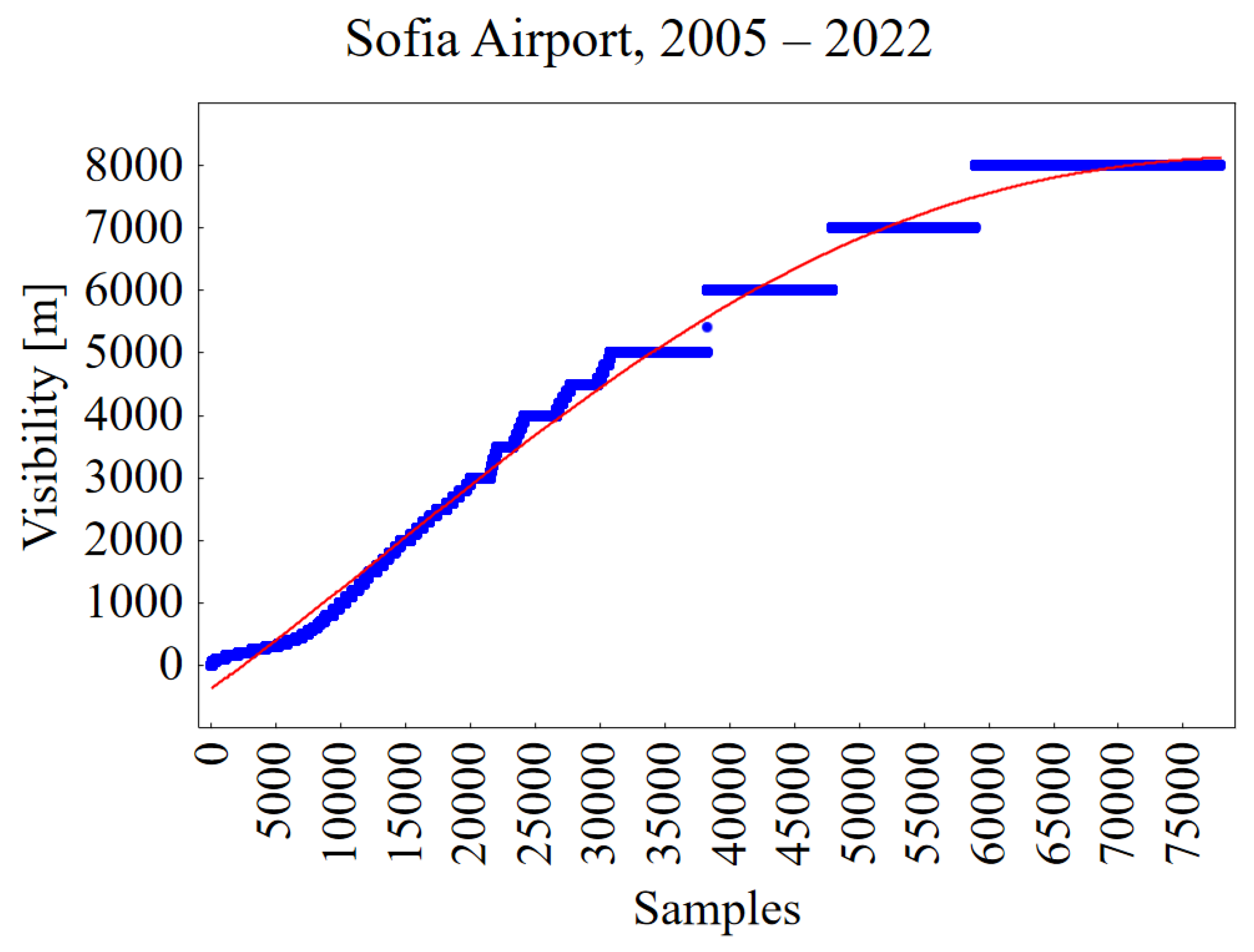
The algorithm requires numerical values for every variable; thus, the cloud coverage is transformed from a string to numerical values between 0 and 1. When wind direction is reported as “variable”, it is replaced by the most frequent value. A parameter “dew-point deficit” is added to the data by subtracting the dew point from the temperature in order to have an indicator for the humidity, which is not part of the METAR. The date is converted to the day of the year to represent seasonal variations. Data normalization using MinMax Scaler is applied for all variables. Taking into account that METAR messages encode the visibility above 9000 m as 9999, ML models will not benefit from these reports, because they fail to establish a connection between the visibility and all the other parameters. Therefore, only observations with visibility below 8000 m are included and only when the reported present weather is fog, mist, or none, which results in 77,788 METAR observations (24.7% of the total). The visibility observations in ascending order are presented in Figure 2. An almost linear distribution is seen with slight changes in the angle of the curve above 500 m and above 4000 m visibility. Approximately 10,000 observations have visibility below 1000 m, nearly 28,000 observations have visibility between 1000 and 5000 m, and almost 40,000 reports have visibility between 6000 and 8000 m.

2.3. Random Forest Model

The random forest model is a supervised ensemble ML algorithm (Breiman [24]). The algorithm splits the dataset into training and testing subsets. The training set of data is used to build multiple decision trees using the bootstrap method (Efron [25]). Each tree uses a subsample of the training set and builds itself by looking for optimal performance based on mean squared error and a threshold-based approach over a subset of data features. The RF model is suitable for both classification and regression tasks. In this study, it is used for regression tasks since we look for visibility values.

RF Model Training

Cross-validation is applied with 100 setups to obtain the optimal parameter values. Table 1 presents the parameters used for configuring the model. Two thousand trees are built by the model during training and then used for testing. The max features parameter is the number of features to consider when looking for the best split. The square root of the total number of features is used for the max features parameter. Max depth is a measure of how deep the tree is from its root node to its deepest leaf node. The min samples parameter represents the minimum number of data samples required to split an internal node. The data are split into 70% training set and 30% for testing. The variables used for building the trees are day, hour, wind speed, wind direction, first layer cloud base and coverage, temperature, dew point, temperature deficit, and pressure. The model was configured and compiled using the scikit-learn library (Pedregosa et al. [26]).

2.4. Long Short-Term Memory Model (LSTM)

The LSTM network (Hochreiter and Schmidhuber [27]) is a recurrent neural network model that is designed to solve the issue of vanishing gradients (Rumelhart et al. [28]). This issue is caused by the rapid increase or decrease in gradients in gradient-based optimization algorithms during the training stage. In the case of LSTM, the optimization algorithm is the rate of change of the loss function, which measures the difference between the predictions and the actual values. The model is suitable for time series forecasting because it has a three gate mechanism and an additional feature—the memory cell. The gates are named update, forget, and output. The update gate controls new information, which is stored in the memory cell, and the forget gate is responsible for storing only the important information. The output gate combines the current and previous input (one step prior) state of the hidden layer. These two are combined with the current state of the memory cell to produce the network output that will also be used for the input of the next hidden layer. This mechanism is able to effectively detect long-term dependencies and non-linear relationships in time series.

LSTM Model Training

The same data pre-processing is applied as for the RF model. The data set is again split into 70% for training and 30% for testing. In Table 2 the LSTM setup parameters are given. The number of units (neurons) is set to 150, and the number of time steps available as input is 12, which is 6 h. The adaptive moment estimation (Adam) optimizer (Kingma and Ba [29]) is used for loss function minimization during training. The learning rate of the optimizer is exponential decay starting from 0.01 and reduced by 0.9 for every 10,000 steps. The rectified linear activation function (ReLU) is used to control the model output, making sure that the predictions have only positive values. In this study, the mean squared error is used as a loss function, and the number of epochs is set to 10. The model was configured and compiled using the Keras API (Chollet et al. [30]).

2.5. R2, MAE, RMSE

The coefficient of determination (R2) is calculated to evaluate model performance. This coefficient is an assessment of how well the true visibility values are likely to be predicted by the model. The possible values are between 0 and 1, where 1 is the perfect prediction, and 0 is for no relationship between the input and the output of the model. Mean absolute error (MAE) and root mean squared error (RMSE) are also used to evaluate model accuracy. While R2 provides an indication of precision, MAE and RMSE give a measurement of the average of the differences between predictions and observations (MAE) and a measurement of the magnitude of these differences (RMSE). All three metrics are calculated using the scikit-learn library (Pedregosa et al. [26]) with the following formulae:
R 2 ( y , y ^ ) = 1 1 n ( y n y ^ n ) 2 1 n ( y n y ¯ ) 2
M A E ( y , y ^ ) = 1 n × 1 n | y n y ^ n |
R M S E ( y , y ^ ) = 1 n × 1 n ( y n y ^ n ) 2
where n is the number of samples, y is the observation, y ^ is the prediction from the model, and y ¯ is the mean of y.

2.6. POD, FAR, CSI, TSS

Probability of detection (POD), false alarm ratio (FAR), critical success index (CSI), and true skill statistic (TSS) are calculated to provide an additional evaluation of model performance. These scores are used for classification tasks; thus, a necessary transformation of the results is applied. The predicted and observed visibility is divided into three classes—fog (0 < visibility < 1000 m), mist (1000 m ≤ visibility ≤ 5000 m), and NIL (visibility > 5000 m). The classification matrix is obtained, and the metrics are calculated by the formulae:
(1) Probability of detection (POD, [31]):
P O D = T P T P + F N
(2) False alarm ratio (FAR, [31]):
F A R = F P F P + T N
(3) Critical success index (CSI, [31]):
C S I = T P T P + F P + F N
(4) True skill statistic (TSS, [31]):
T S S = T P T P + F N F P F P + T N
where T P is the number of correctly estimated fog registrations, F N is the number of misses (undetected fog registrations), T N is the number of correctly estimated no-fog registrations, and F P is the number of incorrectly estimated fog registrations (fog was estimated by the model but not observed). POD presents the percentage of correct fog estimations, and FAR is the rate of incorrect fog estimations. C S I and T S S , similar to R2, measure the accuracy of the models.
The visualizations of fog characteristics and model performance were carried out with Statistica Software (Sta [32]), Matplotlib (Hunter [33]) and Seaborn (Waskom [34]) libraries.

3. Results

3.1. Sofia Airport Fog Characteristics: 2005–2022

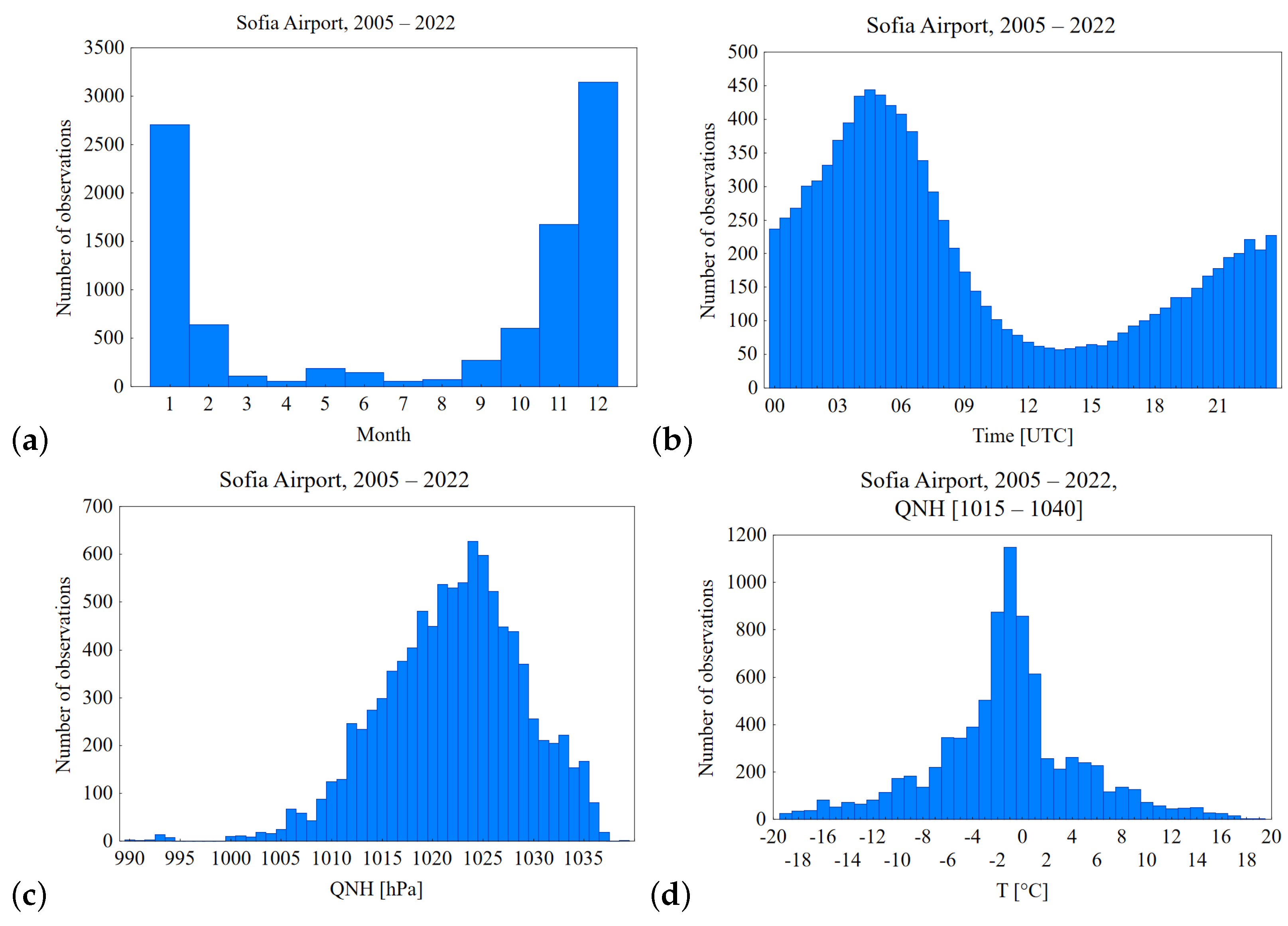
A seasonal distribution of fog observations is presented in Figure 3a, which confirms that fog appears mostly in winter, but also a small secondary peak is seen for the months May and June. The secondary peak of fog occurrences is related to the annual maximum of the monthly rate of precipitation, which is usually convective precipitation. This type of precipitation can be caused either by daytime heating or as a result of passing cold fronts. After rain, soil moisture and air humidity are increased in addition to calm weather and clear sky, and temperature can drop enough for fog to form. The diurnal distribution of fog observations is shown in Figure 3b where it is clearly seen that the maximum is around 04-05 UTC just before sunrise, and that is when the minimum temperatures are observed. The measured sea level pressure (Figure 3c) during fog is high, with a maximum of 1024 hPa. Whilst the majority of cases reported are above a pressure of 1013 hPa, cases reported below that value are not negligible. While the majority of fog observations are associated with anticyclonic weather, there are a number of fog cases caused by an approaching cyclone from W-SW or a low-gradient pressure field and a weak flow at 850 hPa pressure level from W-SW, as reported in Penov et al. [15]. Figure 3d presents the temperatures at which fog is reported for the pressure interval 1015–1040 hPa. The maximum is at −1 °C, and most of the cases are grouped around it in the interval from −6 °C to 2 °C. With the temperature dropping below −6 °C, ice deposition takes place, and this is why fog occurrence is less likely.
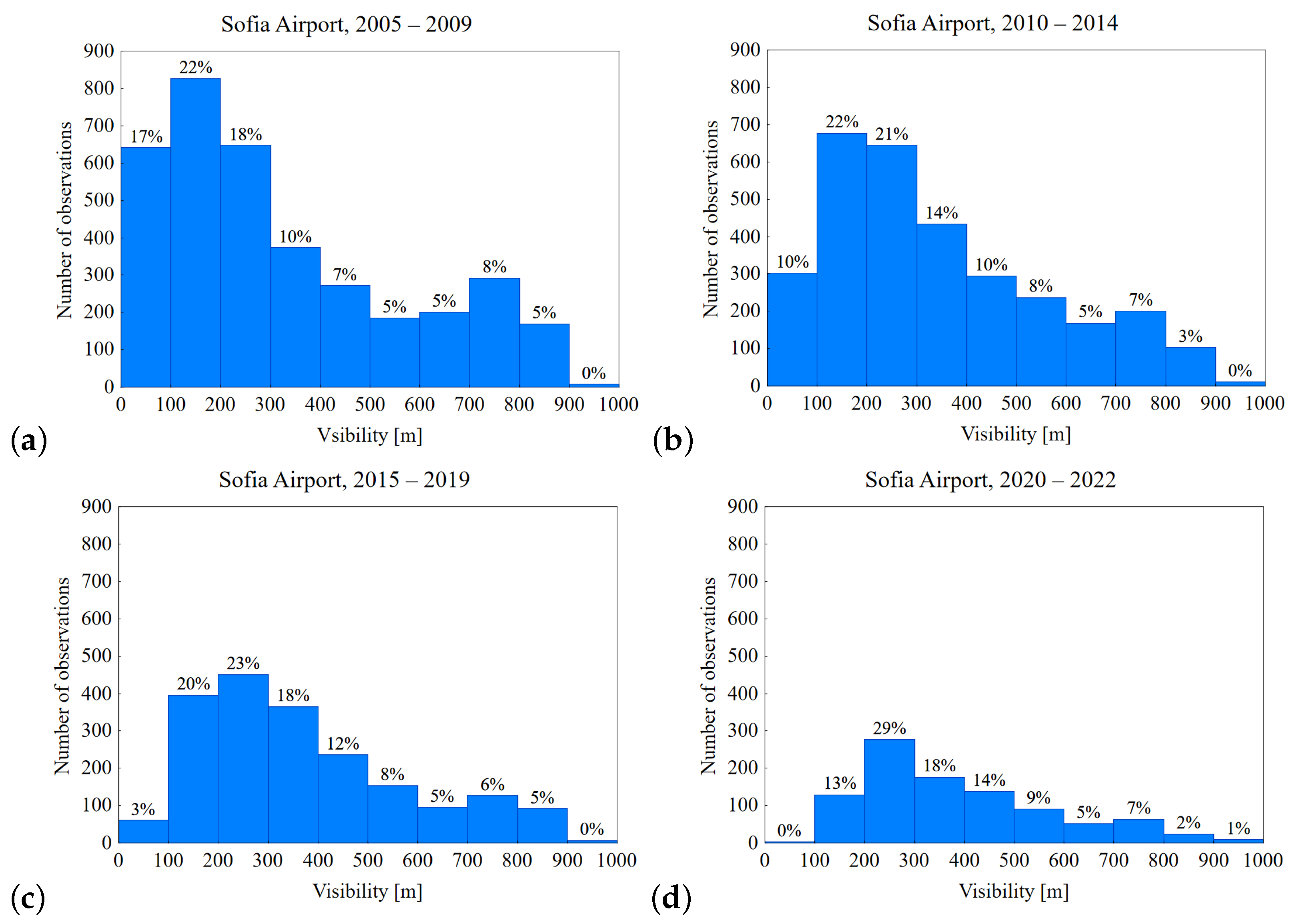
The frequency of fog observations (Figure 4) for the period 2005–2022 is divided into three consecutive periods of five years and one period of three years (2005–2009, 2010–2014, 2015–2019, and 2020–2022). Every next period shows an overall decrease in the number of fog observations, but, more interestingly, the maximum of the fog observations is shifted towards the higher visibility range. While for the first period, the maximum is in the range of 100–200 m with 57% of all cases below 300 m visibility (Figure 4a), the maximum for the last period is in the range of 200–300 m with 42% of the cases below 300 m and practically no observations below 100 m (Figure 4d). This behavior could be explained by the closure of the biggest metallurgical company in Bulgaria in 2010, located about 8 km from the airport in the NE direction. Circulation (Vautard and Yiou [35], Stoev et al. [36]) and climate changes (Maurer et al. [37], Hunova et al. [38]) can also be factors.
Wind speed and direction are very important parameters of fog formation. Figure 5a presents the distribution of reported wind direction when fog is observed. For 33% of the observations, wind direction is reported, while for 46% of the data, the wind direction is stated as “variable”, i.e., for the last 10 min before the METAR is issued the variations in the direction exceed 180°. Based on that, a wind rose is presented in Figure 5b for the cases when wind direction is reported. The predominant direction is from E-SE, and wind speed is mostly below 5 kt. This result is expected as moisture sources are located eastward from the airport, and therefore a weak wind from that direction is increasing fog probability.

3.2. Random Forest and LSTM Visibility Estimation

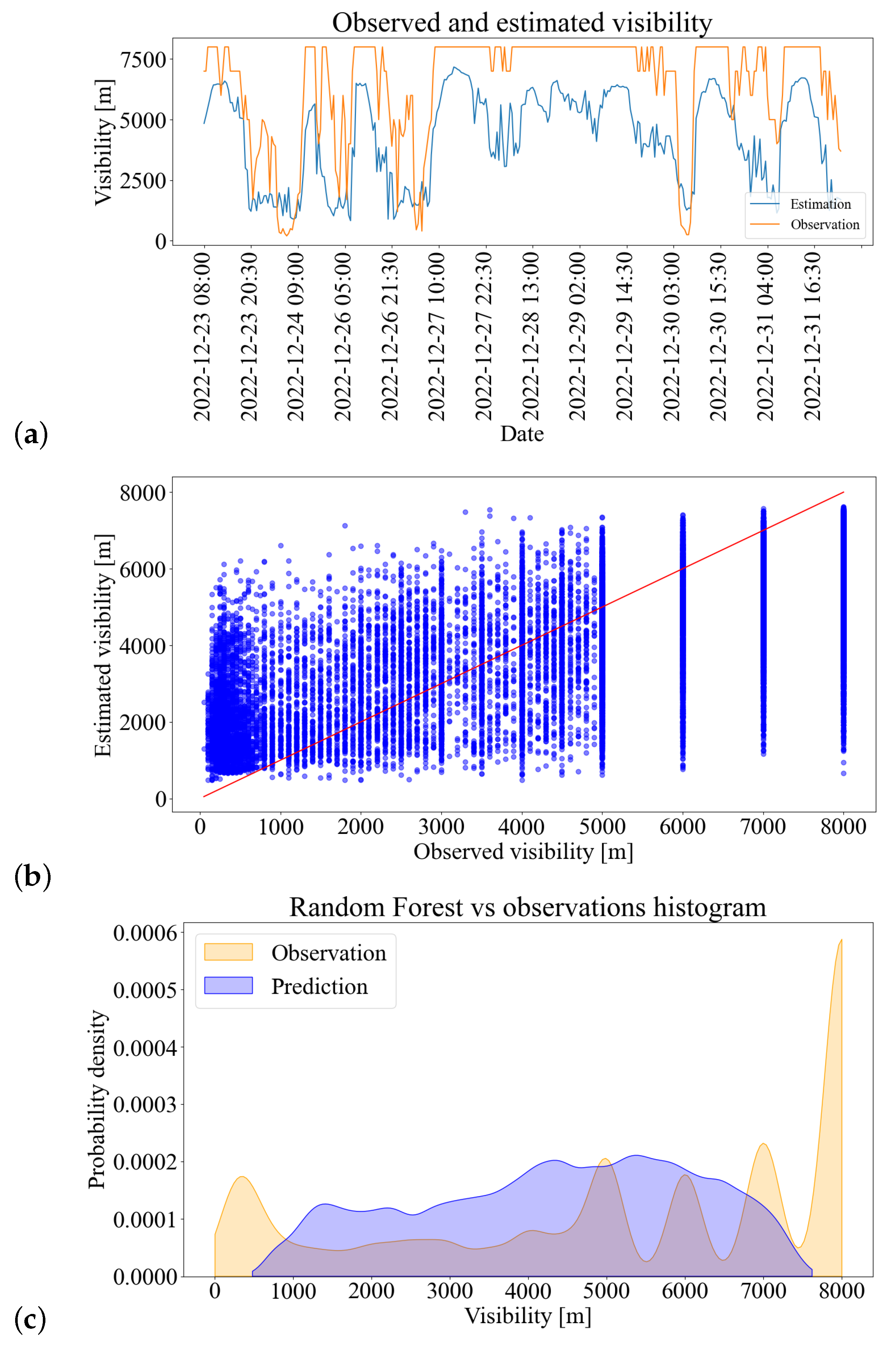
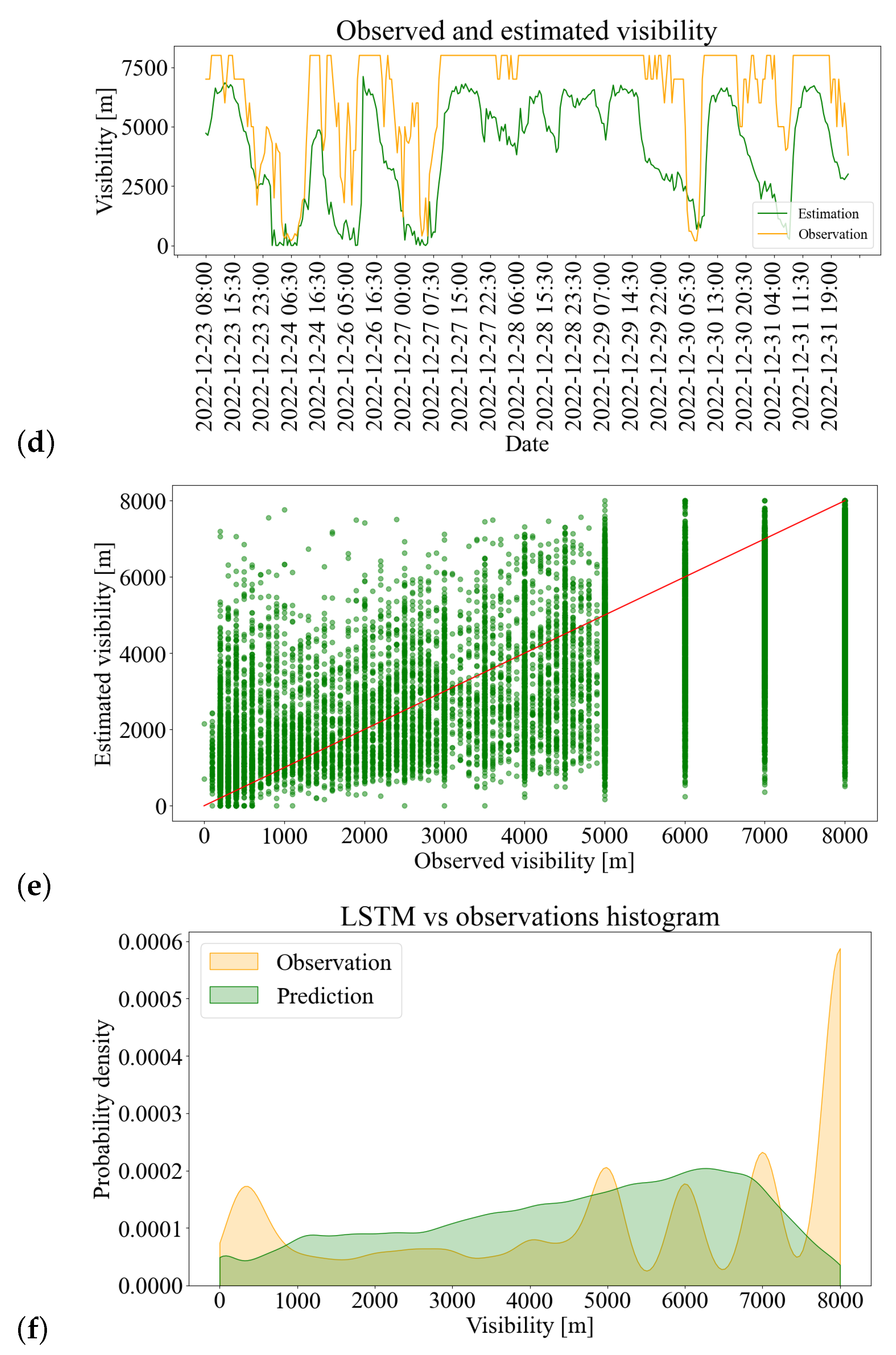
The RF and LSTM models are used to predict visibility on given 11 features for 30% of the data. Figure 6a,d present predictions and observations for the end of the test data. The period includes three fog cases and demonstrates the ability of the models to track the complex nature of fog formation and dissipation. Figure 6b is the scatter plot for the relationship between predicted and observed visibility. It is clearly seen that low visibility is overestimated, whilst high visibility is underestimated. Identical results are obtained by the LSTM model (Figure 6d,e). The histograms of visibility (Figure 6c,f) show that both models have problems predicting the lowest and highest visibility from the data, although LSTM performs better for visibility below 1000 m.

3.2.1. Results Post-Processing and Model Evaluation

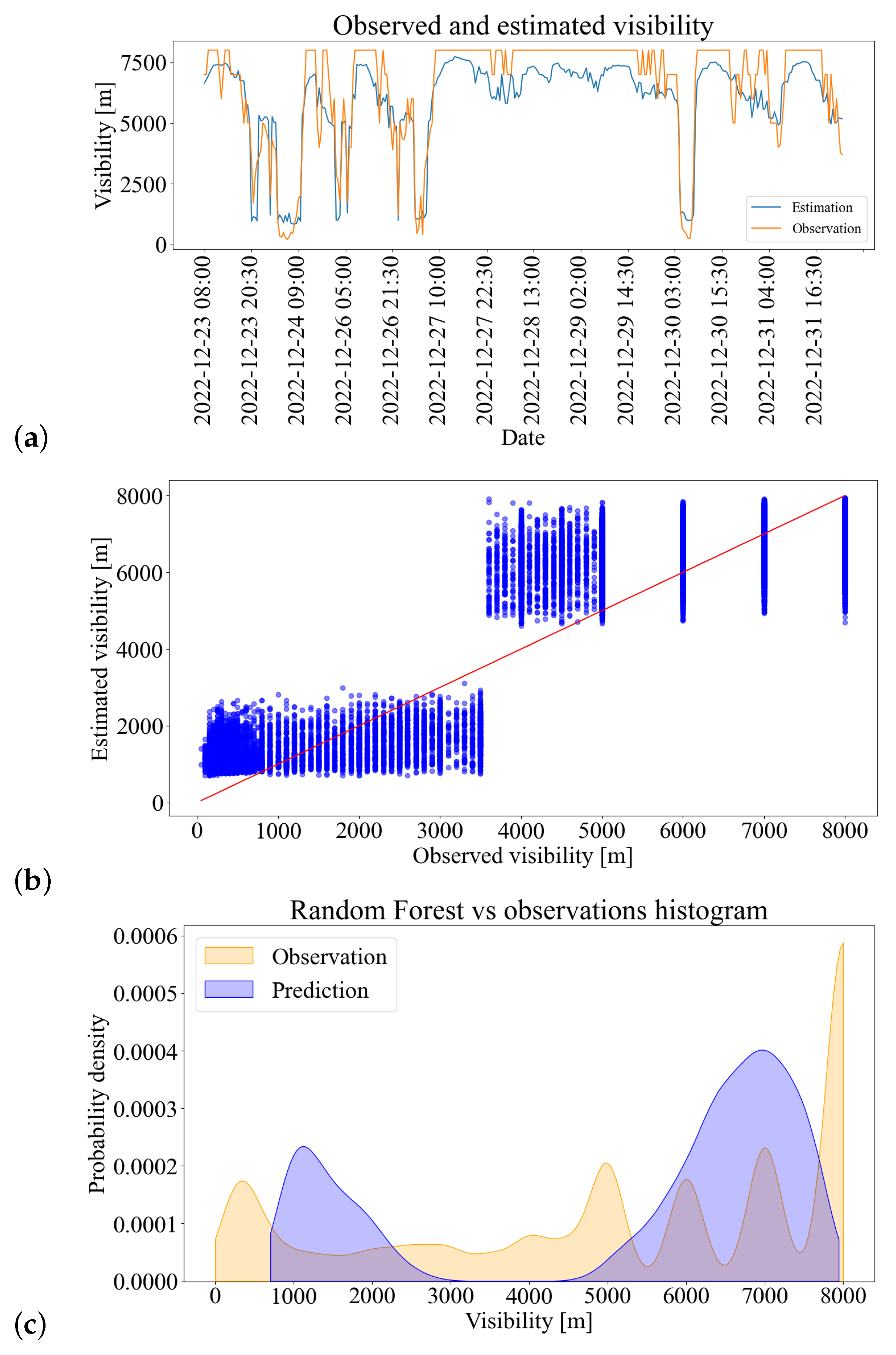
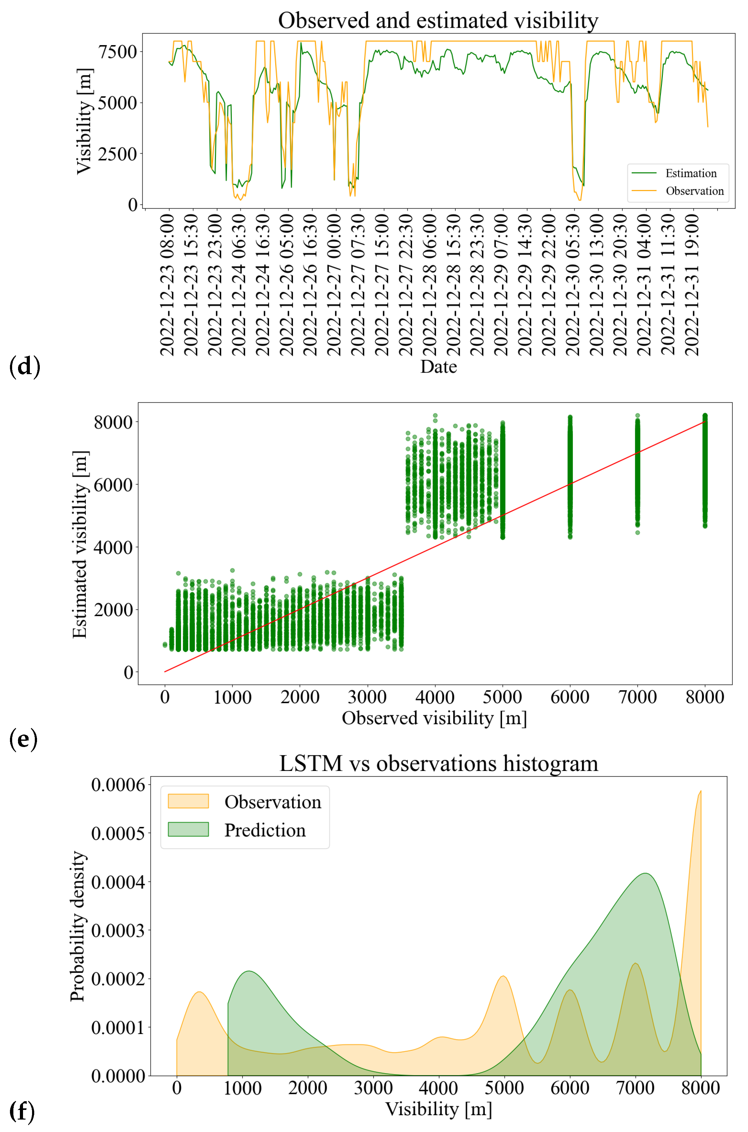
Both positive and negative biases are common issues for estimating visibility (Kim et al. [19]). Thus, a double correction of the results from the RF and LSTM models is made with a linear function (Kim et al. [39]). The data are split into two sets for visibility below 3500 m and above 3500 m. The function was derived by applying linear regression between predictions and actual visibility values. The equation was then applied to the predictions from the model in order to obtain corrected values. The correction functions are as follows:
RF
V i s i b i l i t y [ m ] = 0.33× y + 516
V i s i b i l i t y [ m ] = 0.47× y + 4339
LSTM
V i s i b i l i t y [ m ] = 0.33× y + 759
V i s i b i l i t y [ m ] = 0.44× y + 4418
where y is the predicted value. Equations (8) and (10) are applied for y <= 3500 m and Equations (9) and (11) for the cases where y > 3500 m. By applying different corrections for the cases with observed visibility below and above 3500 m for the RF and 4000 m for the LSTM models, the bias is significantly reduced, and as seen on the time series (Figure 7a,d) the predictions are more accurate. The scatter plot after the post-processing (Figure 7b,e) indicates that there will be a rapid change in the values when the threshold of 3500 m is passed. This behavior is in line with the observed rapid change in visibility during fog onset and dissipation. Visibility between 5000 and 1000 m changes very quickly, as seen in Figure 7a,d. The histograms of the visibility (Figure 7c,f) show that the predictions are shifted and clustered in two separate areas for low and high visibility, which corresponds better with the observations.
Evaluation of the performance of the models is given in Table 3. As is seen, R2 increases significantly from 0.38 to 0.81 for the RF and from 0.44 to 0.82 for the LSTM models after post-processing for correcting model bias. For the RF model, MAE has a 44% decrease from 1752 m down to 984 m and RMSE has a 45% decrease from 2123 m down to 1178 m. For LSTM, MAE has a 40% decrease from 1600 m down to 955 m, and RMSE has a 43% decrease from 2024 m down to 1154 m. MAE and RMSE retain a similar relationship, with RMSE being 21% higher before and 20% higher after for the RF model, while for LSTM RMSE is 27% higher before and 21% higher after the post-processing. The similarity between MAE and RMSE values means that there are no outliers that significantly affect the squared error.
The classification matrices for the post-processed RF and LSTM models are presented in Figure 8a,b, and classification metrics are presented in Table 4. The obtained POD and FAR scores are low because of the positive bias in the predictions in the low-visibility range as is seen in Figure 7c,f. The FAR values are around 1% for all configurations which is an indication of the ability of the algorithms to correctly recognize the low-visibility conditions.

3.2.2. Feature Importance

RF also provides a calculation of the importance of each input variable for the model. The results are summarized in Table 5. According to the algorithm, the most important parameter (34%) is the FSI followed by the dew-point deficit (23%), as both of them are a measure of relative humidity. This result is in agreement with Choi et al. [40], where they also find relative humidity as the most important input parameter for visibility estimation according to the RF model. Its top position is expected as without saturation of the water vapor, fog formation is impossible regardless of the other parameters. Cloud base is the third most important parameter (11%). This parameter is more difficult to interpret because it provides information about the outgoing Earth long wave radiation balance, whereas low clouds directly affect visibility. Air temperature is at fourth place, and as presented in Figure 3d the number of fog observations and the temperature have an obvious relationship. The importance of wind speed and direction is also well-defined and can be seen in Figure 5b. Although, according to the model, wind direction is not important along with the pressure, hour, and cloud coverage, they have their impact on fog development, but their role remains small probably because of the ensemble process of making a prediction. For example, clouds are very important for whether or not the temperature will drop enough for saturation, but most fog cases occur when there is a clear sky.

4. Conclusions

This work investigated the fog characteristics at Sofia Airport for the period 2005–2022 using METAR observations, as well as visibility estimation capability of two machine-learning models. The main fog characteristics were studied for the first time for the airport with the highest traffic in Bulgaria. The fog is mainly during the autumn and winter seasons, but there is a secondary peak during May and June. Fog occurs predominantly when the temperature is between −6 and 2 °C and the pressure is high with a maximum number of fog occurrences at 1024 hPa. For the studied period, there is a clear tendency of decrease in the number of fog observations, and the maximum is shifting towards higher visibility.
The two machine-learning models (RF and LSTM) were built to estimate the visibility on 11 meteorological parameters. Both models achieve similar performance by detecting the increasing or decreasing visibility tendency, but an overall positive bias is observed for the low-visibility spectrum (below 2500–3000 m) and a negative bias for the rest of the spectrum. Post-processing with linear regression was applied, which improved the models’ performance significantly. The FSI is ranked as the most important parameter with 34%, followed by the dew-point deficit with 23%, and the cloud base with 11%.
The machine-learning approach for visibility-related regression tasks shows very good capability for learning the complex and nonlinear characteristics of fog formation and dissipation. The visibility range of up to 8000 m is of high interest for aviation as the ML algorithm teaches itself about the conditions before fog initiation. This provides a lead time for air traffic authorities to prepare for a likely upcoming fog. Although similar studies show a noticeable difference in the performance between ensemble ML and neural networks, in our work their difference is very small. This could be as a result of the large dataset, which is enough for both models to train themselves equally. Although in this work only an estimation was made, a continuation of the study will be to test the performance in case studies using NWP data as input in order to predict visibility. The LSTM model will be used for recursive forecasting, aiming at producing a tool to help operational forecasters in aviation issue timely fog warnings.

Author Contributions

Conceptualization N.P. and G.G.; methodology, N.P.; software, N.P.; validation, N.P.; formal analysis, N.P.; writing—original draft preparation, N.P.; writing—review and editing, all authors; visualization, N.P. All authors have read and agreed to the published version of the manuscript.

Funding

Guergana Guerova acknowledges funding by the European Union NextGenerationEU through the National Recovery and Resilience Plan of the Republic of Bulgaria, project No. BG-RRP-2.004-0008.

Data Availability Statement

The data are not publicly available.

Acknowledgments

We are very grateful to Georgi Peev from BULATSA, for providing the METAR observations.

Conflicts of Interest

The authors declare no conflict of interest. The funders had no role in the design of this study; in the collection, analyses, or interpretation of data; in the writing of the manuscript; or in the decision to publish the results.

References

  1. Gultepe, I.; Sharman, R.; Williams, P.D.; Zhou, B.; Ellrod, G.; Minnis, P.; Trier, S.; Griffin, S.; Yum, S.S.; Gharabaghi, B.; et al. A review of high impact weather for aviation meteorology. Pure Appl. Geophys. 2019, 176, 1869–1921. [Google Scholar] [CrossRef]
  2. Belo-Pereira, M.; Santos, J. A persistent wintertime fog episode at Lisbon airport (Portugal): Performance of ECMWF and AROME models. Meteorol. Appl. 2016, 23, 353–370. [Google Scholar] [CrossRef]
  3. Liu, D.; Niu, S.; Yang, J.; Zhao, L.; Lü, J.; Lu, C. Summary of a 4-year fog field study in northern Nanjing, Part 1: Fog boundary layer. Pure Appl. Geophys. 2012, 169, 809–819. [Google Scholar] [CrossRef]
  4. Román-Cascón, C.; Yagüe, C.; Sastre, M.; Maqueda, G.; Salamanca, F.; Viana, S. Observations and WRF simulations of fog events at the Spanish Northern Plateau. Adv. Sci. Res. 2012, 8, 11–18. [Google Scholar] [CrossRef]
  5. Smith, D.K.; Renfrew, I.A.; Dorling, S.R.; Price, J.D.; Boutle, I.A. Sub-km scale numerical weather prediction model simulations of radiation fog. Q. J. R. Meteorol. Soc. 2021, 147, 746–763. [Google Scholar] [CrossRef]
  6. Jia, X.; Quan, J.; Zheng, Z.; Liu, X.; Liu, Q.; He, H.; Liu, Y. Impacts of anthropogenic aerosols on fog in North China Plain. J. Geophys. Res. Atmos. 2019, 124, 252–265. [Google Scholar] [CrossRef]
  7. Yan, S.; Zhu, B.; Huang, Y.; Zhu, J.; Kang, H.; Lu, C.; Zhu, T. To what extents do urbanization and air pollution affect fog? Atmos. Chem. Phys. 2020, 20, 5559–5572. [Google Scholar] [CrossRef]
  8. Boutle, I.; Price, J.; Kudzotsa, I.; Kokkola, H.; Romakkaniemi, S. Aerosol–fog interaction and the transition to well-mixed radiation fog. Atmos. Chem. Phys. 2018, 18, 7827–7840. [Google Scholar] [CrossRef]
  9. Bergot, T.; Escobar, J.; Masson, V. Effect of small-scale surface heterogeneities and buildings on radiation fog: Large-eddy simulation study at Paris–Charles de Gaulle airport. Q. J. R. Meteorol. Soc. 2015, 141, 285–298. [Google Scholar] [CrossRef]
  10. Shao, N.; Lu, C.; Jia, X.; Wang, Y.; Li, Y.; Yin, Y.; Zhu, B.; Zhao, T.; Liu, D.; Niu, S.; et al. Radiation fog properties in two consecutive events under polluted and clean conditions in the Yangtze River Delta, China: A simulation study. Atmos. Chem. Phys. 2023, 23, 9873–9890. [Google Scholar] [CrossRef]
  11. Arun, S.; Chaurasia, S.; Misra, A.; Kumar, R. Fog Stability Index: A novel technique for fog/low clouds detection using multi-satellites data over the Indo-Gangetic plains during winter season. Int. J. Remote Sens. 2018, 39, 8200–8218. [Google Scholar] [CrossRef]
  12. Holtslag, M.; Steeneveld, G.; Holtslag, A. Fog forecasting: “Old fashioned” semi-empirical methods from radio sounding observations versus “modern” numerical models. In Proceedings of the 5th International Conference on Fog, Fog Collection and Dew (FOGDEW2010), Münster, Germany, 25–30 July 2010. [Google Scholar]
  13. Song, Y.; Yum, S.S. Development and verification of the fog stability index for Incheon international airport based on the measured fog characteristics. Atmosphere 2013, 23, 443–452. [Google Scholar] [CrossRef]
  14. Stoycheva, A.; Evtimov, S. Studying the fogs in Sofia with Cherni vrah-Sofia Stability Index. Bulg. Geophys. J. 2014, 40, 23–32. [Google Scholar]
  15. Penov, N.; Stoycheva, A.; Guerova, G. Fog in Sofia 2010–2019: Objective circulation classification and fog indices. Atmosphere 2023, 14, 773. [Google Scholar] [CrossRef]
  16. Lui, G.N.; Hon, K.K.; Liem, R.P. Weather impact quantification on airport arrival on-time performance through a Bayesian statistics modeling approach. Transp. Res. Part C Emerg. Technol. 2022, 143, 103811. [Google Scholar] [CrossRef]
  17. Schultz, M.; Reitmann, S.; Alam, S. Predictive classification and understanding of weather impact on airport performance through machine learning. Transp. Res. Part C Emerg. Technol. 2021, 131, 103119. [Google Scholar] [CrossRef]
  18. Bari, D.; Bergot, T.; Tardif, R. Fog Decision Support Systems: A Review of the Current Perspectives. Atmosphere 2023, 14, 1314. [Google Scholar] [CrossRef]
  19. Kim, J.; Kim, S.H.; Seo, H.W.; Wang, Y.V.; Lee, Y.G. Meteorological characteristics of fog events in Korean smart cities and machine learning based visibility estimation. Atmos. Res. 2022, 275, 106239. [Google Scholar] [CrossRef]
  20. Castillo-Botón, C.; Casillas-Pérez, D.; Casanova-Mateo, C.; Ghimire, S.; Cerro-Prada, E.; Gutierrez, P.; Deo, R.; Salcedo-Sanz, S. Machine learning regression and classification methods for fog events prediction. Atmos. Res. 2022, 272, 106157. [Google Scholar] [CrossRef]
  21. Peláez-Rodríguez, C.; Pérez-Aracil, J.; de Lopez-Diz, A.; Casanova-Mateo, C.; Fister, D.; Jiménez-Fernández, S.; Salcedo-Sanz, S. Deep learning ensembles for accurate fog-related low-visibility events forecasting. Neurocomputing 2023, 549, 126435. [Google Scholar] [CrossRef]
  22. Dewi, R.; Harsa, H. Fog prediction using artificial intelligence: A case study in Wamena Airport. J. Phys. Conf. Ser. 2020, 1528, 012021. [Google Scholar] [CrossRef]
  23. Bartok, J.; Šišan, P.; Ivica, L.; Bartoková, I.; Malkin Ondík, I.; Gaál, L. Machine learning-based fog nowcasting for aviation with the aid of camera observations. Atmosphere 2022, 13, 1684. [Google Scholar] [CrossRef]
  24. Breiman, L. Random forests. Mach. Learn. 2001, 45, 5–32. [Google Scholar] [CrossRef]
  25. Efron, B. Bootstrap methods: Another look at the jackknife annals of statistics. Ann. Statist. 1979, 7, 1–26. [Google Scholar] [CrossRef]
  26. Pedregosa, F.; Varoquaux, G.; Gramfort, A.; Michel, V.; Thirion, B.; Grisel, O.; Blondel, M.; Prettenhofer, P.; Weiss, R.; Dubourg, V.; et al. Scikit-learn: Machine Learning in Python. J. Mach. Learn. Res. 2011, 12, 2825–2830. [Google Scholar]
  27. Hochreiter, S.; Schmidhuber, J. Long short-term memory. Neural Comput. 1997, 9, 1735–1780. [Google Scholar] [CrossRef] [PubMed]
  28. Rumelhart, D.E.; Hinton, G.E.; Williams, R.J. Learning representations by back-propagating errors. Nature 1986, 323, 533–536. [Google Scholar] [CrossRef]
  29. Kingma, D.; Ba, J. Adam: A method for stochastic optimization. In Proceedings of the 3rd International Conference for Learning Representations (iclr’15), San Diego, CA, USA, 7–9 May 2015; Volume 500. [Google Scholar]
  30. Chollet, F. Keras. 2015. Available online: https://keras.io/ (accessed on 24 September 2023).
  31. Hanssen, A.; Kuipers, W. On the Relationship between the Frequency of Rain and Various Meteorological Parameters. (With Reference to the Problem of Objective Forecasting); Koninklijk Nederlands Meteorologisch Instituut: Utrecht, The Netherlands, 1965. [Google Scholar]
  32. StatSoft Inc. Statistica (Data Analysis Software System), 6th ed.; StatSoft Inc.: Tulsa, OK, USA, 2001; p. 150. Available online: www.statsoft.com (accessed on 23 April 2023).
  33. Hunter, J.D. Matplotlib: A 2D graphics environment. Comput. Sci. Eng. 2007, 9, 90–95. [Google Scholar] [CrossRef]
  34. Waskom, M.L. Seaborn: Statistical data visualization. J. Open Source Softw. 2021, 6, 3021. [Google Scholar] [CrossRef]
  35. Vautard, R.; Yiou, P. Control of recent European surface climate change by atmospheric flow. Geophys. Res. Lett. 2009, 36. [Google Scholar] [CrossRef]
  36. Stoev, K.; Post, P.; Guerova, G. Synoptic circulation patterns associated with foehn days in Sofia in the period 1979–2014. IdŐJÁRÁS/Q. J. Hung. Meteorol. Serv. 2022, 126, 545–566. [Google Scholar] [CrossRef]
  37. Maurer, M.; Klemm, O.; Lokys, H.L.; Lin, N.H. Trends of fog and visibility in Taiwan: Climate change or air quality improvement? Aerosol Air Qual. Res. 2019, 19, 896–910. [Google Scholar] [CrossRef]
  38. Hunova, I.; Brabec, M.; Maly, M.; Valerianova, A. Long-term trends in fog occurrence in the Czech Republic, Central Europe. Sci. Total. Environ. 2020, 711, 135018. [Google Scholar] [CrossRef] [PubMed]
  39. Kim, B.Y.; Cha, J.W.; Chang, K.H.; Lee, C. Visibility prediction over South Korea based on random forest. Atmosphere 2021, 12, 552. [Google Scholar] [CrossRef]
  40. Choi, W.; Park, J.; Kim, D.; Park, J.; Kim, S.; Lee, H. Development of two-dimensional visibility estimation model using machine learning: Preliminary results for South Korea. Atmosphere 2022, 13, 1233. [Google Scholar] [CrossRef]
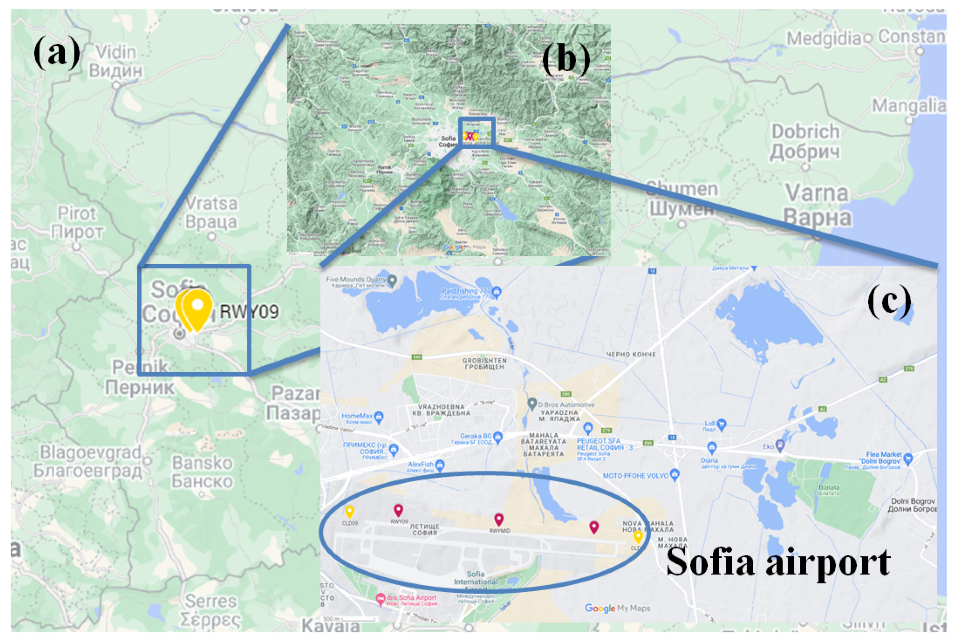
Figure 1. Map of Bulgaria (a) with double zoom over the Sofia Plain (b) and over the airport area (c). Red and yellow markers indicate the sensor’s locations.
Remotesensing 15 04799 g001
Figure 2. Visibility distribution in ascending order. The red line is a polynomial fit.
Remotesensing 15 04799 g002
Figure 3. Sofia Airport fog characteristics. (a) Monthly number of fog observations, (b) diurnal distribution, (c) fog observations as a function of pressure, and (d) fog observations and air temperature for the 1015–1039 hPa pressure interval.
Remotesensing 15 04799 g003
Figure 4. Number of fog observations and visibility ranges for the period (a) 2005–2009, (b) 2010–2014, (c) 2014–2019, and (d) 2020–2022.
Remotesensing 15 04799 g004
Figure 5. (a) Distribution of the observations with reported wind direction, variable direction, and calm. (b) Sofia Airport wind rose when fog is reported.
Remotesensing 15 04799 g005
Figure 6. (a) RF and (d) LSTM visibility estimation. (b) Correlation between observations and predictions for RF and (e) for LSTM. The red line points to the perfect match. (c,f) Visibility histogram of observations and predictions.
Remotesensing 15 04799 g006aRemotesensing 15 04799 g006b
Figure 7. (a) Random forest and (d) LSTM visibility estimation after post-processing. (b,e) Correlation between observations and predictions after post-processing. The red line points to the perfect match. (c,f) Visibility histogram of observations and predictions after post-processing.
Remotesensing 15 04799 g007aRemotesensing 15 04799 g007b
Figure 8. Classification matrices for (a) RF* and (b) LSTM*.
Remotesensing 15 04799 g008
Table 1. Random forest options.
ParameterTreesMax FeaturesMax DepthMin Samples
Value2000sqrt1010
Table 2. LSTM parameters.
ParameterUnitsStepsOptimizerLearning RateActivationLoss FunctionEpochs
Value15012AdamExponential decayReLUMean squared error10
Table 3. RF and LSTM performance assessment. RF* and LSTM* stand for the post-processed predictions.
R2MAE [m]RMSE [m]
RF0.3817522123
RF*0.819841178
LSTM0.4416002024
LSTM*0.829551154
Table 4. POD, FAR, CSI, and TSS for fog calculated for the RF and LSTM models. RF* and LSTM* stand for the post-processed predictions.
RFRF*LSTMLSTM*
POD [%]12302937
FAR [%]0.71.70.91
CSI [%]11272735
TSS [%]11282836
Table 5. RF feature importance.
VariableImportance
FSI0.34
Dew-point deficit0.23
Cloud base0.11
Temperature0.09
Wind speed0.08
Day of year0.06
Dew point0.04
Hour0.02
Pressure0.02
Wind direction0.01
Cloud coverage0.01
Disclaimer/Publisher’s Note: The statements, opinions and data contained in all publications are solely those of the individual author(s) and contributor(s) and not of MDPI and/or the editor(s). MDPI and/or the editor(s) disclaim responsibility for any injury to people or property resulting from any ideas, methods, instructions or products referred to in the content.