Integrated 1D, 2D, and 3D CNNs Enable Robust and Efficient Land Cover Classification from Hyperspectral Imagery

Abstract

Convolutional neural networks (CNNs) have recently been demonstrated to be able to substantially improve the land cover classification accuracy of hyperspectral images. Meanwhile, the rapidly developing capacity for satellite and airborne image spectroscopy as well as the enormous archives of spectral data have imposed increasing demands on the computational efficiency of CNNs. Here, we propose a novel CNN framework that integrates one-dimensional (1D), two-dimensional (2D), and three-dimensional (3D) CNNs to obtain highly accurate and fast land cover classification from airborne hyperspectral images. To achieve this, we first used 3D CNNs to derive both spatial and spectral features from hyperspectral images. Then, we successively utilized a 2D CNN and a 1D CNN to efficiently acquire higher-level representations of spatial or spectral features. Finally, we leveraged the information obtained from the aforementioned steps for land cover classification. We assessed the performance of the proposed method using two openly available datasets (the Indian Pines dataset and the Wuhan University dataset). Our results showed that the overall classification accuracy of the proposed method in the Indian Pines and Wuhan University datasets was 99.65% and 99.85%, respectively. Compared to the state-of-the-art 3D CNN model and HybridSN model, the training times for our model in the two datasets were reduced by an average of 60% and 40%, respectively, while maintaining comparable classification accuracy. Our study demonstrates that the integration of 1D, 2D, and 3D CNNs effectively improves the computational efficiency of land cover classification with hyperspectral images while maintaining high accuracy. Our innovation offers significant advantages in terms of efficiency and robustness for the processing of large-scale hyperspectral images.

1. Introduction

Hyperspectral remote sensing technology, or image spectroscopy, utilizes hyperspectral sensors for the simultaneous imaging of the target area using continuously subdivided bands [1]. Compared to multispectral imaging, hyperspectral imaging contains more information, allowing it to accurately detect the properties of ground features and use them in some tasks, especially in land cover classification [2,3]. Recently, numerous small and cost-effective hyperspectral sensors have been introduced for aviation drones [4,5]. Meanwhile, several space-borne hyperspectral imagers, such as Zhuhai-1 [6], PRISMA [7], and EnMAP [8], have also been launched. The acquisition of large volumes of hyperspectral data requires fast and efficient analytical methods [9]. However, the high spectral dimensionality and increasing spatial resolution generate large volumes of hyperspectral data, thereby posing numerous challenges in image classification [10,11].

The convolutional neural network (CNN) offers a promising solution for hyperspectral image classification, efficiently extracting spectral–spatial features and making it a prevalent algorithm today [12,13]. Previous studies have shown that CNN methods are capable of achieving high classification accuracy in hyperspectral image classification tasks [14,15,16]. There are three widely used hyperspectral classification methods based on dimensional CNN methods, i.e., one-dimensional (1D), two-dimensional (2D), and three-dimensional (3D) CNNs [17,18]. Within this context, 1D CNN is responsible for extracting spectral details, while 2D CNN is tailored for spatial information extraction [19,20]. Conversely, 3D CNN, comprising 3D convolution kernels, extracts both spatial and spectral attributes [21]. Although 3D CNN excels at spatial–spectral feature fusion, its complexity can elevate network computing costs [22]. Given the surging data volumes, complex models often fall short in classification accuracy and computational efficiency [14,23]. Consequently, integrated CNNs have been proposed to overcome this problem [24].

Integrated CNNs are recognized as an effective approach, utilizing a combination of two CNNs, specifically from 1D, 2D, and 3D CNNs, for accurate land cover classification results from hyperspectral images [25,26]. For instance, Roy et al. [26] introduced an integrated CNN method called HybridSN that used 3D CNNs to derive spatial–spectral joint features from three dimensions using hyperspectral 3D cubes, while also employing 2D CNNs to process spatial details from spectral images. HybridSN offers enhanced computational efficiency and improved classification accuracy compared to 3D CNN [26]. However, HybridSN lacks the capacity to fully extract spectral features from the hyperspectral data and performs poorly in classifying certain land cover types [27,28]. Zhang et al. [29] also introduced an integrated CNN model, called 3D-1D CNN, which used a 3D CNN to derive high-level spectral–spatial semantic information, followed by a 1D CNN to learn abstract spectral details. This approach has been shown to improve CNN’s computational performance in the classification of certain land cover types from hyperspectral images [29]. However, the 3D-1D CNN method fails to effectively account for spatial characteristics and is not suitable for multiclass classification tasks.

In the real world, hyperspectral data typically contain various categories of objects, with some exhibiting distinct spatial feature differences and others being more distinguishable based on spectral features. Consequently, the simple integration of two CNNs cannot achieve optimal accuracy and efficiency results, particularly in scenarios involving multiclass classification tasks and handling large volumes of hyperspectral images [30,31]. Here, for the first time, we propose a novel CNN framework that integrates 1D, 2D, and 3D CNNs to achieve highly accurate and computationally efficient land cover classification results from airborne hyperspectral images. We firstly assess the new model using two open datasets (the Indian Pines dataset and the Wuhan University dataset), and secondly, we compare the performance of our method against four existing CNN methods (1D CNN, 2D CNN, 3D CNN, and HybridSN).

2. Materials and Methods

2.1. Description of the Dataset

We selected two hyperspectral image datasets to assess the performance of our method, including the Indian Pines dataset (https://www.ehu.eus/ccwintco/index.php?title=Hyperspectral_Remote_Sensing_Scenes, accessed on 1 October 2022), and the Wuhan University dataset (http://rsidea.whu.edu.cn/resource_WHUHi_sharing.htm, accessed on 16 October 2022) [32,33]. The two datasets differ in spectral resolution, spatial resolution, data volume, and land cover types.

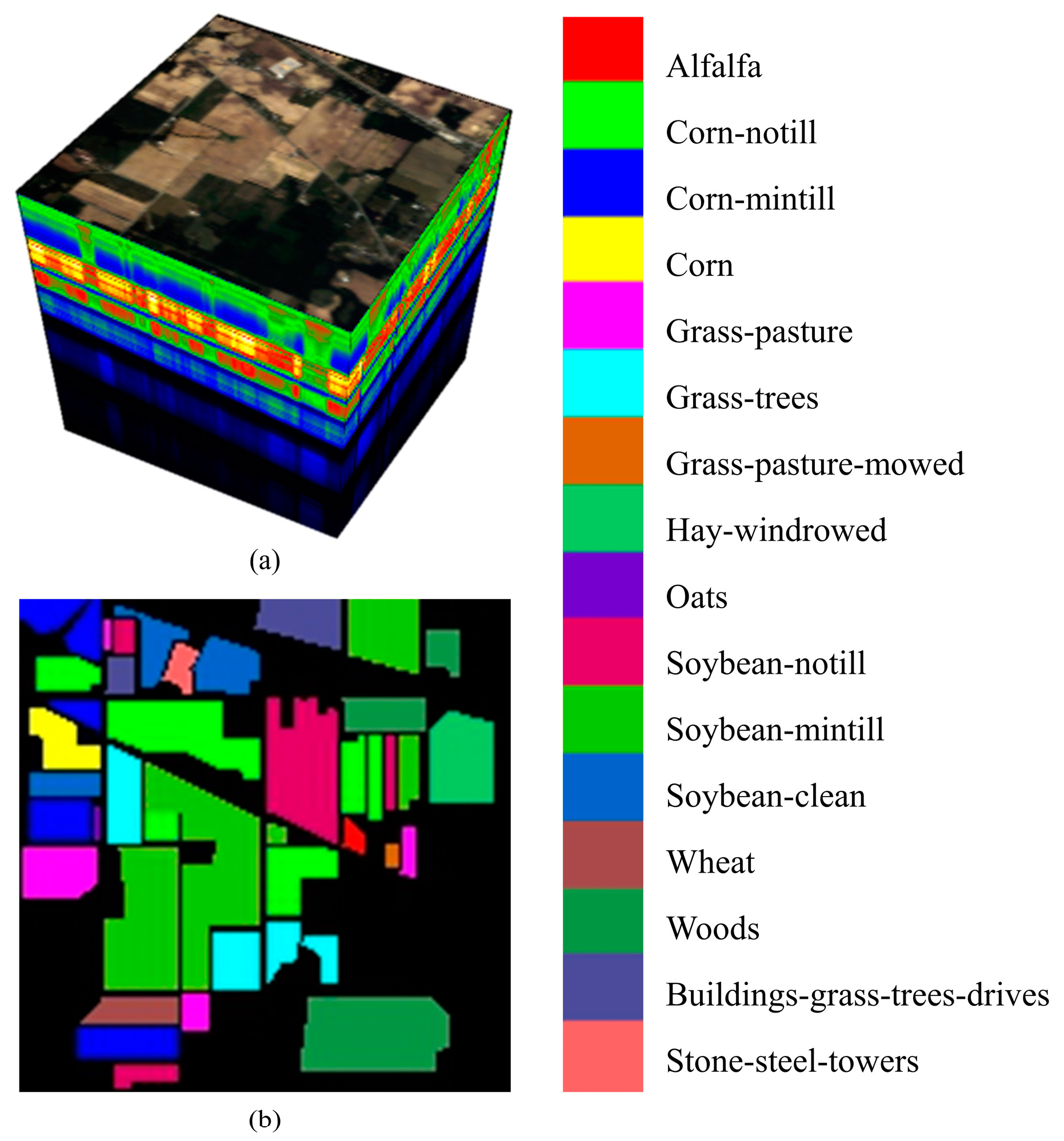
2.1.1. The Indian Pines Dataset

The Indian Pines dataset, acquired in 1992 using the Airborne Visible/Infrared Imaging Spectrometer (AVIRIS), covers a test region in Indiana, USA. The dataset comprises 145 × 145 pixels, covering 224 spectral bands from 400 to 2500 nm, at a 20 m spatial resolution. With a data volume of 5.67 MB, it includes 16 land cover classes.

Table 1. The land cover classes within the Indian Pines dataset, detailing training and test samples for each.

No.	Land Cover Classes	Total Samples	Training Samples	Test Samples
1	Alfalfa	46	14	32
2	Corn-notill	1428	428	1000
3	Corn-mintill	830	249	581
4	Corn	237	71	166
5	Grass-pasture	483	145	338
6	Grass-trees	730	219	511
7	Grass-pasture-mowed	28	8	20
8	Hay-windrowed	478	143	335
9	Oats	20	6	14
10	Soybean-notill	972	292	680
11	Soybean-mintill	2455	737	1719
12	Soybean-clean	593	178	415
13	Wheat	205	62	144
14	Woods	1265	380	886
15	Buildings-grass-trees-drives	386	116	270
16	Stone-steel-towers	93	28	65

provides the specifics on these classes and the distribution of the training and test samples, while Figure 1 depicts the true color composite 3D hyperspectral image cube alongside the ground reference map.

2.1.2. The Wuhan University Dataset

The Wuhan University dataset was obtained using the unmanned aerial vehicle (UAV)-borne visible/near-infrared Headwall Nano-Hyperspec hyperspectral systems in Hanchuan City, Hubei Province, China on 17 June 2016. The dataset features images measuring 1217 × 303 pixels, encompassing 274 spectral bands within a 400 to 1000 nm wavelength range. With a 0.109 m spatial resolution, the data size amounts to 262 MB. The dataset primarily encompasses 16 land cover classes, predominantly varied croplands.

Table 2. The land cover classes within the Wuhan University dataset detailing training and test samples for each.

No.	Land Cover Classes	Total Samples	Training Samples	Test Samples
1	Strawberry	44,735	13,421	31,315
2	Cowpea	22,753	6826	15,927
3	Soybean	10,287	3086	7201
4	Sorghum	5353	1606	3747
5	Water spinach	1200	360	840
6	Watermelon	4533	1360	3173
7	Greens	5903	1771	4132
8	Trees	17,978	5393	12,585
9	Grass	9469	2841	6628
10	Red roof	10,516	3155	7361
11	Gray roof	16,911	5073	11,838
12	Plastic	3679	1104	2575
13	Bare soil	9116	2735	6381
14	Road	18,560	5568	12,992
15	Bright object	1136	341	795
16	Water	75,401	22,620	52,781

details these classes along with their associated training and test samples. Figure 2 displays a true color composite 3D hyperspectral image cube and its associated ground reference map.

2.2. Related Works

In this section, we will highlight some significant works related to the integrated CNNs topics. Figure 3 illustrates the convolution architecture of the related CNN frameworks, i.e., 1D, 2D, and 3D CNNs. The input hyperspectral data is presented in the form of a three-dimensional cube, which can be converted into three different feature representations: 1D spectral, 2D spatial, or 3D spectral–spatial features.

One-dimensional CNN models only use 1D convolution kernels to analyze the input 1D spectral features [34]. Each pixel vector is represented as 1D data and is then processed via the 1D CNN to derive deeper spectral insights [35]. Given that this data processing hinges solely on spectral signatures, discerning between various land covers becomes challenging due to the spectral mixing effect [36].

Two-dimensional CNN models only utilize 2D convolution kernels to extract abstract spatial information from 2D spatial features [26]. This approach brings clarity to the spatial dynamics among neighboring pixels [37]. However, there is a possibility that the model might sometimes neglect pivotal spectral correlations [26].

Three-dimensional CNN models employ 3D convolution kernels to discern local variations in the spectral–spatial dimensions of 3D hyperspectral image features [38]. Their approach renders them particularly effective for hyperspectral image tasks [25]. However, 3D CNN can instigate challenges such as increased computational complexity, susceptibility to overfitting, gradient vanishing, and explosion, limiting their widespread application [29].

Recently, integrated CNNs have garnered considerable attention, resulting in enhanced classification accuracy [26]. Two integrated CNN models have been devised to address the limitations of earlier models: the fusion of 3D with 1D CNNs, and the union of 3D with 2D CNNs [25,26]. Consequently, the layered application of different CNNs can capture more descriptive information vital for hyperspectral image classification tasks. Nonetheless, the classification precision for individual species remains suboptimal [17].

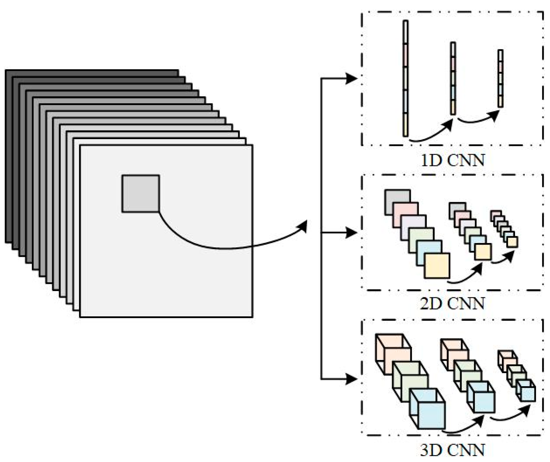
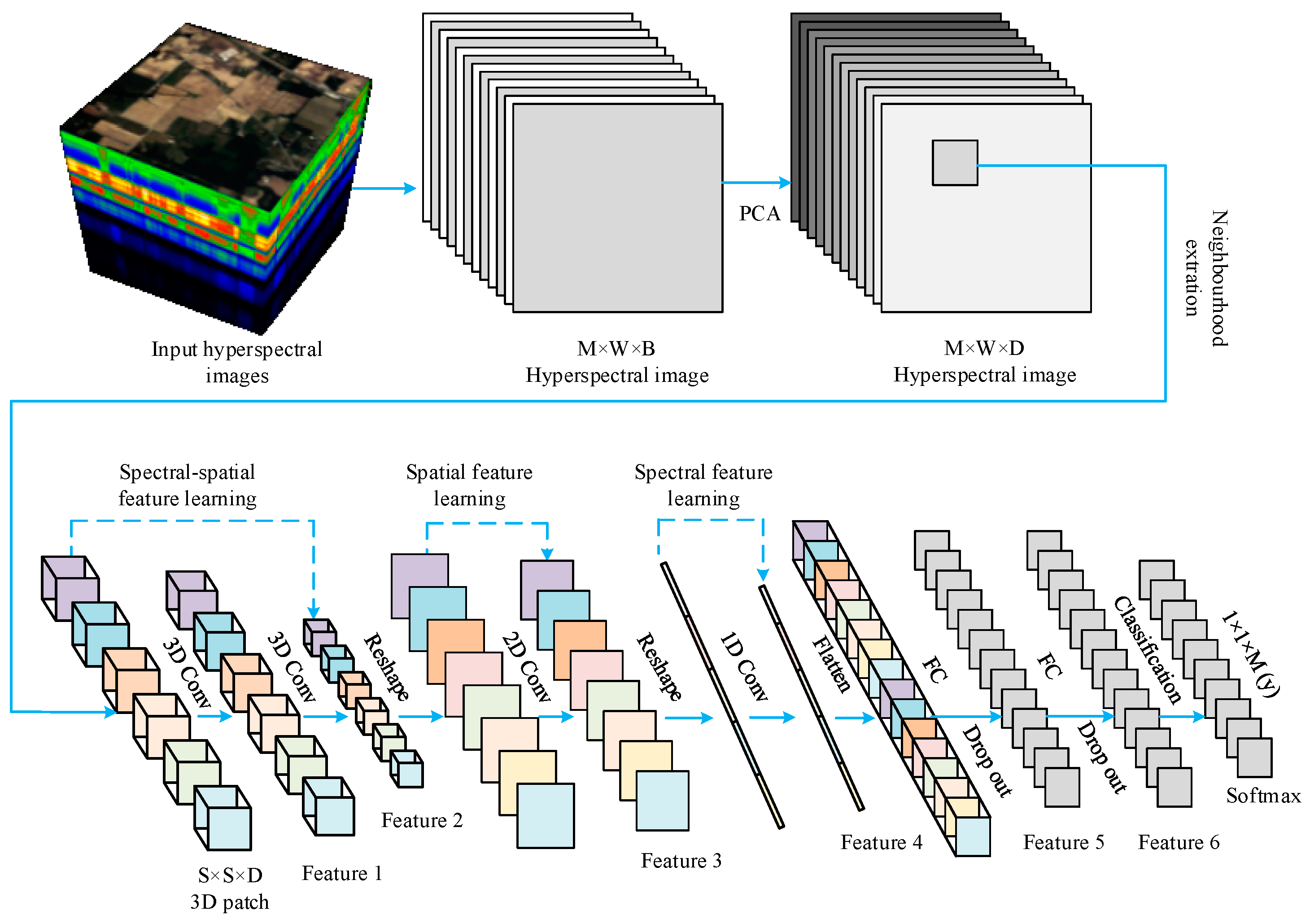
2.3. Proposed Integrated 1D, 2D and 3D CNNs (IntegratedCNNs)

Figure 4 illustrates the architecture of the IntegratedCNNs. The IntegratedCNNs model uses all three types of dimensional CNNs (i.e., 1D, 2D, and 3D CNNs) in a sequential manner to extract and simplify diverse features from the hyperspectral image cube. First, 3D patches are extracted from the 3D hyperspectral data to serve as the input for the model. Subsequently, 3D CNNs derive combined spectral–spatial information from these 3D patches. During this procedure, every feature map in the 3D convolutional layer interacts with multiple spectrograms, thereby integrating both spectral and spatial data for a richer understanding. Subsequently, a 2D CNN refines this by extracting higher-order spatial details from the 3D CNN output maps. Then, a 1D CNN, built on top of the 2D CNN, enhances the learning of spatial representation. Finally, the classification is performed using the information derived from the preceding stages. The IntegratedCNNs preserves the spectral–spatial joint information extraction capability of the 3D CNN, while also substituting some of the 3D convolution stages with 2D and 1D convolution processes. Based on the convolution architecture of 1D, 2D, and 3D CNNs, the IntegratedCNNs achieves both efficient feature extraction and improved computational efficiency compared to traditional 3D CNN methods [39,40].

In our proposed IntegratedCNNs approach, the input hyperspectral images cube is represented by $I\in R^{H\times W\times B}$. Here, $H$ represents the height,$W$ stands for the width, and $B$ indicates the spectral band count of an individual pixel. Within the input map $I$, each pixel carries spectral details associated with a label vector $y\in 1\times 1\times M$, with M indicating the number of classification categories for ground objects. In addition, the multitude of narrow spectral bands in the hyperspectral data present challenges for the classification tasks [41,42]. To tackle this, principal component analysis (PCA) has been employed for dimensionality reduction [31]. By applying PCA, the high-dimensional input data of $I$ undergoes a reduction in spectral bands, resulting in the output data being represented by $X\in R^{M\times W\times D}$. Here, $D$ corresponds to the count of spectral bands following the reduction in dimensionality. For the experiments conducted on the Wuhan University dataset, the optimal number of components after the PCA dimensionality reduction was 15. Conversely, for the Indian Pines dataset, this number was 30. Then, the data cube $X$ is further segmented into overlapping 3D patches, represented as $P\in R^{S\times S\times D}$; here, $S\times S$ is the spatial extent of each patch. The label of a patch $P$ is assigned based on its central pixel. Subsequently, the 3D patches are sequentially processed through four CNN layers, resulting in the generation of output feature maps 1, 2, 3, and 4. Finally, the classification results are obtained by passing the output feature maps through a flattening layer and then through two fully connected (FC) layers. The flattening layer collapses the input dimensions into a single dimension, thus reshaping the input into a format suitable for the FC layers.

The model parameters were determined from the outcomes of our experiments. Some parameters of the experiments in the Indian Pines dataset were identical to those in the Wuhan University dataset. In the process of the network training, we designated 20 epochs and adopted a convolution window size of 25 × 25 pixels. The experiment results indicated that a learning rate of 0.001 yielded optimal classification outcomes, and this was thus selected for our study. The Indian Pines and Wuhan University datasets were each divided into training (30%) and test (70%) subsets, respectively, as depicted in Table 2 and Table 3. Using the Indian Pines dataset as a reference, the IntegratedCNNs has two 3D convolutional layers, a 2D convolutional layer, and a 1D convolutional layer. In the first step, we used two 3D convolutional layers sizes at 8 × 3 × 3 × 7 × 1 and 16 × 3 × 3 × 5 × 8, respectively. The notation 16 × 3 × 3 × 5 × 8 denotes the use of 16 3D convolution kernels, for convolution calculation, applied to eight 3D input feature maps. The size of the 3D kernels was 3 × 3 × 5, where 3 × 3 represented the spatial convolution size, and 5 represented the spectral convolution size. Similarly, 8 × 3 × 3 × 7 × 1 indicated the application of eight 3D kernels of 3 × 3 × 7 to process an input map. In the second step, we used a 2D convolution layer with dimensions of 32 × 3 × 3 × 320 to process the output maps from the 3D layer. In this configuration, 32 denoted the quantity of 2D convolution kernels, 3 × 3 represented their spatial dimensions, and 320 represented the count of input feature maps. Finally, we employed a 1D convolution layer to optimize the spectral data further. The dimensions of the 1D layer were 64 × 3 × 608, where 64 indicated the total convolution kernels, 3 represented the spectral dimensions of these kernels, and 608 was the count of spectral spectra maps. The final layer contained 16 nodes, aligning with the class count in the Indian Pines dataset. The cumulative trainable parameters for this dataset stood at 5361913. Weights were randomly initialized and subsequently optimized employing the back-propagation algorithm with the Adam optimizer by using the softmax loss [26]. The network was trained without the use of batch normalization, a technique typically employed to expedite training via input layer normalization [43]. Certain parameters were established based on our empirical observations, whereas others were automatically generated by the system. Among these, the system-generated parameters included the input feature map of each convolutional layer and the trainable parameters. For more detailed parameter information regarding the IntegratedCNNs model on the Indian Pines dataset, please refer to

Table A1. A detailed breakdown of our IntegratedCNNs model layers, tailored for the Indian Pines dataset.

Layer	Output Shape	Parameter Count	Kernel
Input layer	(None, 25, 25, 30, 1)	0
Conv3D (1)	(None, 23, 23, 24, 8)	512	8 × (3 × 3 × 7)
Conv3D (2)	(None, 21, 21, 20, 16)	5776	16 × (3 × 3 × 5)
Reshape (1)	(None, 21, 21, 320)	0
Conv2D	(None, 19, 19, 32)	92,192	32 × (3 × 3)
Reshape (2)	(None, 19, 608)	0
Conv1D	(None, 17, 64)	116,800	64 × (3)
Flatten	(None, 1088)	0
Dense (1)	(None, 256)	278,784
Dropout (1)	(None, 256)	0
Dense (2)	(None, 128)	32,896
Dropout (2)	(None, 128)	0
Dense (3)	(None, 16)	2064
Total number of parameters: 5,361,913

. The IntegratedCNNs model code is available at https://github.com/liujinxiang23/IntegratedCNNs, accessed on 1 October 2022.

2.4. Conventional CNN Models

We assessed the performance of our IntegratedCNNs method against four prevalent CNN frameworks, including 1D CNN, 2D CNN, 3D CNN, and HybridSN. To evaluate the classification performance across various CNN models, each model was uniformly designed with four convolutional layers for a fair comparison. The following provides more details about each model. (1) In the 1D CNN model, we employed four convolutional layers with 1D filters of dimensions 8, 16, 32, and 64 to compute the results. The use of smaller filter settings in the initial stages enhances the accuracy. Additionally, the architecture includes a flattening layer, two dropout layers, and two dense layers. (2) For the 2D CNN method, four 2D convolutional layers were applied, with each having a 3 × 3 kernel size. (3) For the 3D CNN model, we used the same network architecture as the IntegratedCNNs method. The only distinction is that the 3D convolutional layers were replaced with 2D and 1D CNN layers. (4) For the HybridSN, we used the model structure proposed in the study by Roy et al. [26] as a reference for our research. The architecture also includes 3D layers and 2D CNN layers.

2.5. Computational Efficiency Assessment

To evaluate the computational efficiency of the IntegratedCNNs approach, we primarily relied on metrics such as training duration and testing duration. In addition, we assessed the convergence efficiency of our method by examining the trends in accuracy and loss across training and validation data collections. We also conduct an ablation study using the Indian Pines dataset to assess different configurations of the model. All experiments were carried out on an NVIDIA GeForce RTX 2080Ti graphics card using the Ubuntu 18 operating system, providing a consistent environment for accurate comparisons and reliable results.

2.6. Accuracy Assessment and Statistical Tests

We utilized three metrics for accuracy assessment in our IntegratedCNNs approach: overall accuracy, average accuracy, and kappa coefficient. Overall accuracy gives the percentage of correct predictions out of the total test samples, serving as an indicator of the model’s general efficacy [44]. On the other hand, average accuracy reflects the mean classification accuracy for each category, allowing us to assess the model’s performance in individual classes [45]. Given the uneven distribution of sample sizes in the two datasets, the classification accuracy may be biased towards the larger categories and neglect the smaller ones [46]. To address this issue, we used the kappa coefficient for consistency testing. The kappa coefficient, which ranges between 0 and 1, measures the model’s consistency, with a higher value signifying better consistency [47]. We also utilized a confusion matrix to assess our model’s performance. Additionally, we applied McNemar’s test to ascertain any statistically significant differences between the performance of the IntegratedCNNs and other CNN models [48].

3. Results

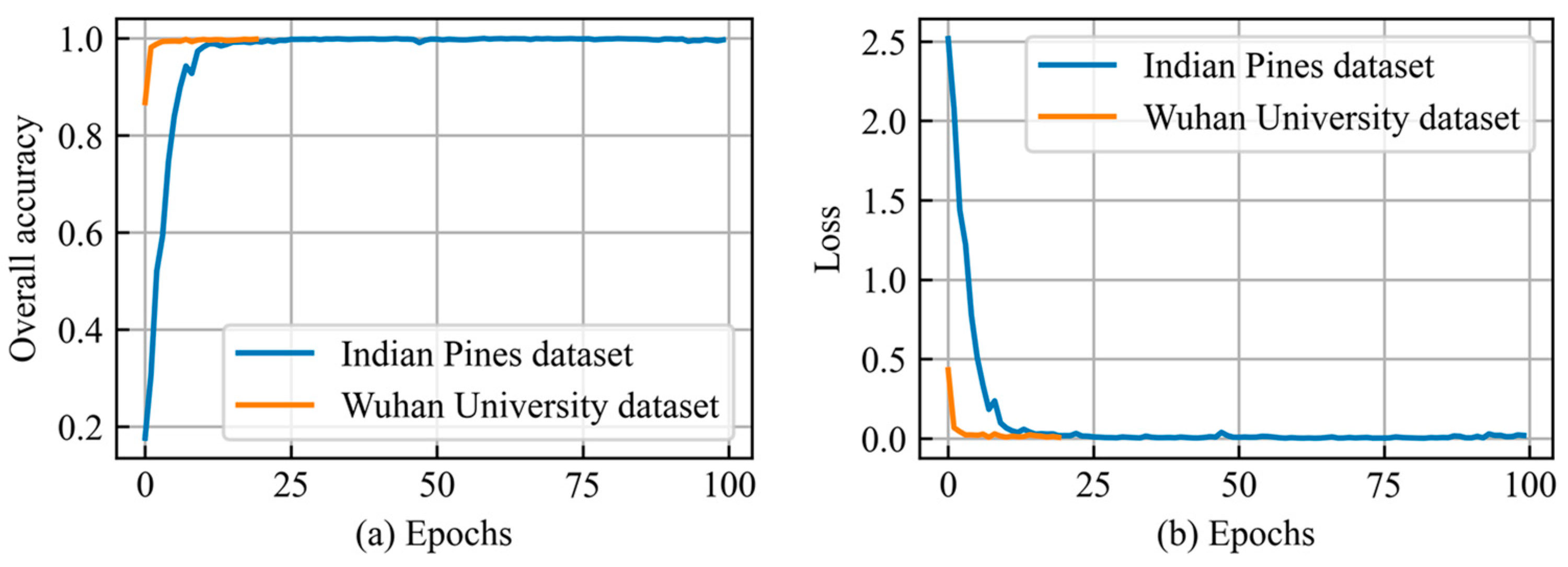
3.1. Performance of the IntegratedCNNs Model

Figure 5 provides a side-by-side comparison of the classified maps produced by the IntegratedCNNs model and the ground reference maps of the Indian Pines and Wuhan University datasets. Overall, the classified maps are in close agreement with the ground reference maps, with only a few misclassified points observed in certain areas.

Figure 6 illustrates the confusion matrix, presenting the accuracy measures of the IntegratedCNNs method across both the Indian Pines and Wuhan University datasets. The predicted pixels are predominantly aligned with the corresponding truth classes, with an insignificant number of misclassified pixels observed.

Figure 7 demonstrates the convergence efficiency of accuracy and loss for the IntegratedCNNs method during 100 epochs of training and validation sets for the Indian Pines and Wuhan University datasets. The convergence of our model was attained in approximately 20 epochs.

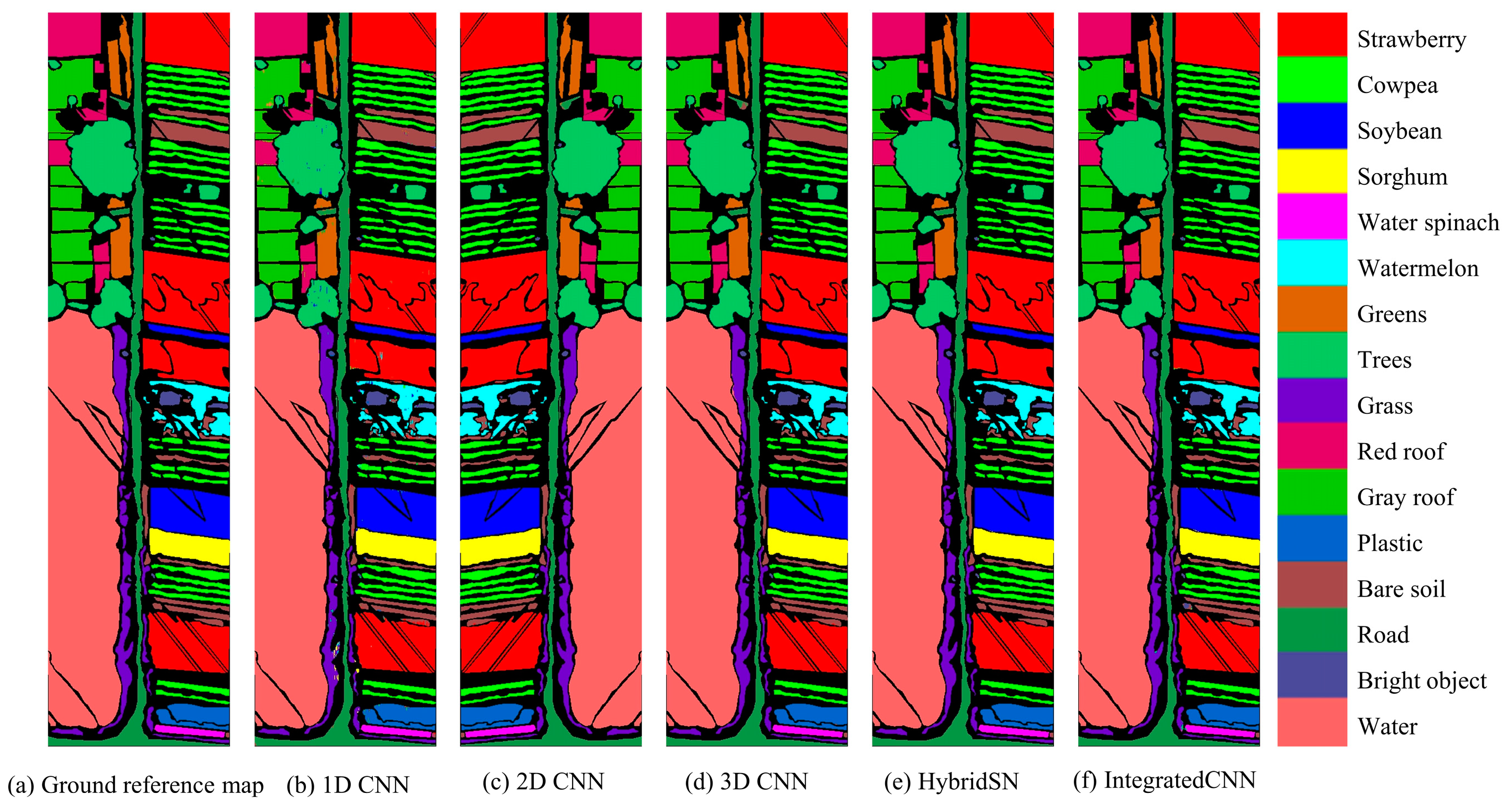
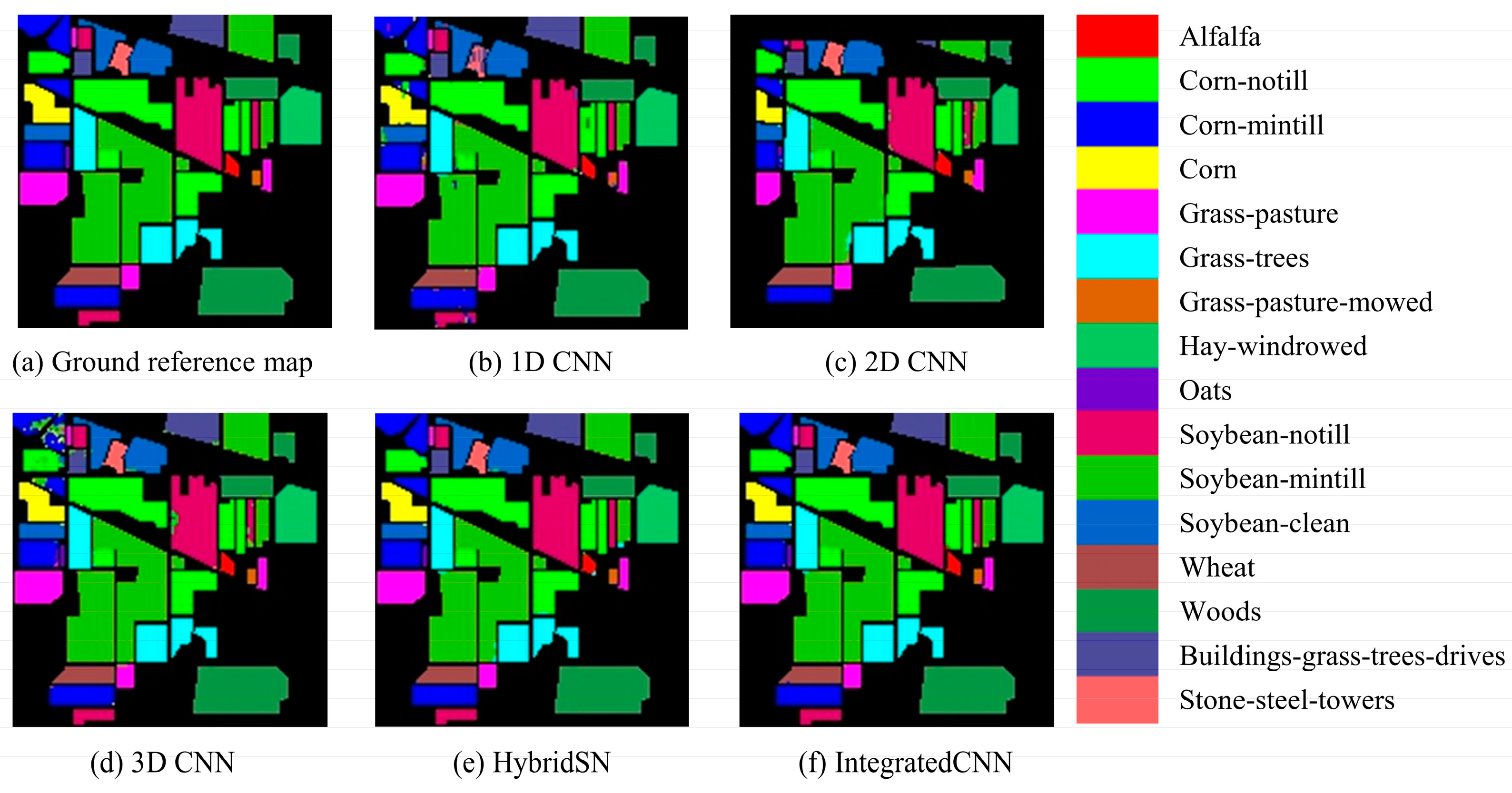
3.2. Model Comparison

Table 3 and

Table 4. McNemar’s test of all compared CNN classifiers (1D CNN, 2D CNN, 3D CNN, HybridSN, and IntegratedCNNs model) in Indian Pines and Wuhan University datasets. Note the values followed by (*) are significant at $\mathsf{\alpha }=0.05$.

	Classifier	1D CNN	2D CNN	3D CNN	HybridSN	IntegratedCNNs
Indian Pines dataset	1D CNN	-
	2D CNN	210.13 *	-
	3D CNN	472.20 *	155.86 *	-
	HybridSN	896.06 *	407.98 *	84.67 *	-
	IntegratedCNNs	957.46 *	459.58 *	196.83 *	32.50 *	-
Wuhan University dataset	1D CNN	-
	2D CNN	770.82 *	-
	3D CNN	1122.80 *	70.45 *	-
	HybridSN	1618.20 *	348.37 *	128.30 *	-
	IntegratedCNNs	1706.59 *	385.41 *	137.54 *	0.12	-

show an overview of the testing accuracy and McNemar’s test for all the compared CNN methods across the Indian Pines and Wuhan University datasets. The IntegratedCNNs consistently outperformed the 1D, 2D, and 3D CNNs in metrics like overall accuracy, average accuracy, and kappa coefficient, with statistically significant results. Furthermore, on the Indian Pines dataset, the accuracy of IntegratedCNNs significantly surpassed that of HybridSN. However, on the Wuhan University dataset, the results of IntegratedCNNs did not exhibit a significant difference compared to that of the HybridSN. More detailed results of the individual class accuracy obtained by all the compared models on the Indian Pines and Wuhan University datasets can be found in

Table A2. The correct rate of each feature sample in each model of the Indian Pines dataset (%).

No.	Land Cover Classes	1D CNN	2D CNN	3D CNN	HybridSN	IntegratedCNNs
1	Alfalfa	78.13	97.37	100.00	87.50	100.00
2	Corn-notill	96.70	98.21	96.70	98.50	99.60
3	Corn-mintill	97.07	99.32	81.93	100.00	100.00
4	Corn	94.58	100.00	100.00	100.00	98.80
5	Grass-pasture	95.86	97.41	98.23	100.00	99.41
6	Grass-trees	99.61	98.66	99.80	100.00	99.61
7	Grass-pasture-mowed	0.00	100.00	100.00	95.00	90.00
8	Hay-windrowed	100.00	100.00	100.00	100.00	100.00
9	Oats	0.00	28.57	100.00	92.86	100.00
10	Soybean-notill	99.56	98.53	95.00	100.00	100.00
11	Soybean-mintill	98.84	98.84	99.77	99.01	99.77
12	Soybean-clean	92.53	97.44	97.83	98.31	99.28
13	Wheat	98.60	100.00	100.00	99.30	98.60
14	Woods	99.55	99.78	98.87	99.77	100.00
15	Buildings-grass-trees-drives	88.15	100.00	94.07	100.00	98.52
16	Stone-steel-towers	38.46	50.538	100.00	100.00	100.00

and

Table A3. The correct rate of each feature sample in each model of the Wuhan University dataset (%).

No.	Land Cover Classes	1D CNN	2D CNN	3D CNN	HybridSN	IntegratedCNNs
1	Strawberry	99.58	99.68	99.96	99.99	99.99
2	Cowpea	99.46	99.57	99.96	99.92	99.97
3	Soybean	99.80	99.92	100.00	100.00	100.00
4	Sorghum	99.41	99.89	99.79	100.00	99.95
5	Water spinach	99.80	99.76	99.88	99.88	100.00
6	Watermelon	95.24	96.19	99.81	99.62	99.72
7	Greens	98.39	97.75	100.00	100.00	99.90
8	Trees	98.39	98.94	99.75	99.90	99.96
9	Grass	97.05	99.46	99.92	99.91	99.94
10	Red roof	98.40	99.01	99.69	99.99	99.93
11	Gray roof	98.70	99.21	99.98	100.00	99.47
12	Plastic	97.68	98.52	100.00	100.00	99.96
13	Bare soil	93.92	95.78	99.31	99.76	99.22
14	Road	99.44	98.71	100.00	99.99	99.38
15	Bright object	91.41	88.93	98.74	97.86	99.75
16	Water	99.94	99.96	100.00	100.00	99.93

, respectively. Visual comparisons between various classification techniques are illustrated in the classification maps provided in Figure A1 and Figure A2.

Table 3. Comparison of testing accuracies (overall, average, and kappa coefficient) across various CNN models on Indian Pines and Wuhan University datasets, with the best results emphasized in bold.

Dataset	Testing Accuracy	1D CNN	2D CNN	3D CNN	HybridSN	IntegratedCNNs
Indian Pines dataset	Overall accuracy (%)	96.54	89.56	96.96	99.33	99.65
	Average accuracy (%)	79.85	94.44	97.64	98.14	98.97
	Kappa coefficient	0.96	0.84	0.97	0.99	1.00
Wuhan University dataset	Overall accuracy (%)	99.02	99.27	99.76	99.92	99.85
	Average accuracy (%)	97.91	98.20	99.43	99.79	99.82
	Kappa coefficient	0.99	0.99	1.00	1.00	1.00

Table 3. Comparison of testing accuracies (overall, average, and kappa coefficient) across various CNN models on Indian Pines and Wuhan University datasets, with the best results emphasized in bold.

Dataset	Testing Accuracy	1D CNN	2D CNN	3D CNN	HybridSN	IntegratedCNNs
Indian Pines dataset	Overall accuracy (%)	96.54	89.56	96.96	99.33	99.65
	Average accuracy (%)	79.85	94.44	97.64	98.14	98.97
	Kappa coefficient	0.96	0.84	0.97	0.99	1.00
Wuhan University dataset	Overall accuracy (%)	99.02	99.27	99.76	99.92	99.85
	Average accuracy (%)	97.91	98.20	99.43	99.79	99.82
	Kappa coefficient	0.99	0.99	1.00	1.00	1.00

Table 5. Training time and testing time of Indian Pines and Wuhan University datasets.

Dataset	Efficiency	1D CNN	2D CNN	3D CNN	HybridSN	IntegratedCNNs
Indian Pines dataset	Training time (s)	44.06	901.20	1477.93	968.71	600.77
	Testing time (s)	5.33	6.51	18.04	20.04	13.37
Wuhan University dataset	Training time (s)	1108.34	4396.18	7935.22	5372.43	3228.42
	Testing time (s)	76.02	27.30	148.71	149.47	114.47

provides insights into the computational efficiency of the compared CNN methods, focusing on training time and testing time. Notably, IntegratedCNNs reported average computational efficiency gains of 60% over 3D CNN and 40% over HybridSN across the Indian Pines and Wuhan University datasets, marking a notable enhancement over the 2D CNN, 3D CNN, and HybridSN methods.

3.3. Ablation Studies

Table 6. Ablation study results of IntegratedCNNs’ 1D, 2D, and 3D CNN configurations on the Indian Pines dataset. Note the CNNs denoted by (✓) are utilized in the models listed on the left.

	3D CNN	2D CNN	1D CNN	Training Time (s)	Testing Times (s)	Overall Accuracy (%)	Average Accuracy (%)	Kappa Coefficient
IntegratedCNNs	✓	✓	✓	600.77	13.37	99.65	98.97	1.00
3D-2D CNN	✓	✓		653.57	13.86	99.55	98.93	0.99
3D-1D CNN	✓		✓	663.51	13.81	99.45	97.05	0.99
2D-1D CNN		✓	✓	114.12	4.17	97.71	91.28	0.97

presents the results of an ablation study focused on the configurations of IntegratedCNNs using the Indian Pines dataset. For clarity in evaluation, the model structures are segmented into four primary categories: IntegratedCNNs (3D-2D-1D CNN), 3D-2D CNN, 3D-1D CNN, and 2D-1D CNN. Notably, the IntegratedCNNs achieves classification accuracy comparable to the 3D-2D CNN and 3D-1D CNN while offering superior computational efficiency.

4. Discussion

Our results demonstrated that the IntegratedCNNs outperformed the other comparative methods, including 1D CNN, 2D CNN, 3D CNN, and HybridSN when considering both classification accuracy and efficiency. Our approach integrated all three CNN models, resulting in robust representations in terms of accuracy and efficiency by combining 1D, 2D, and 3D CNNs into a novel method for integrating the concept of these three classifiers into a single processing chain. Our findings were in alignment with Roy et al. [26] and Zhang et al. [29], who had integrated two CNNs from the options of 1D, 2D, and 3D CNNs, but we obtained a further significant improvement in classification accuracy and efficiency. This success could be attributed to the effective integration strategy of combining the extracted spectral, spatial, and spectral–spatial features from the 1D, 2D, and 3D CNNs respectively, which significantly enhanced the representation ability of hyperspectral images and reduced computing costs.

The integration of CNNs has the potential to improve the accuracy of hyperspectral classification [17,26]. Our study presented compelling evidence that the IntegratedCNNs model outperformed the individual 1D, 2D, and 3D CNN models in metrics such as overall accuracy, average accuracy, and kappa coefficient. Specifically, for the Indian Pines dataset, the IntegratedCNNs posted a notable overall accuracy of 99.65%, surpassing the 1D CNN model at 96.54%, the 2D CNN model at 89.56%, and the 3D CNN model at 96.96% (Table 3). Although the overall accuracy of IntegratedCNNs (99.65%) was only slightly higher than that of HybridSN (99.33%), this difference was statistically significant (Table 4), suggesting a measurable advantage for our proposed model. Parallel findings were observed when applying the IntegratedCNNs model to the Wuhan University dataset. Here, the IntegratedCNNs demonstrated greater statistical significance compared to the 1D, 2D, and 3D CNNs (Table 3 and Table 4). Interestingly, despite a slightly lower overall accuracy of the IntegratedCNNs (99.85%) in comparison to the HybridSN (99.92%), the difference was not statistically significant (Table 4), further affirming the competitive nature of the IntegratedCNNs model in achieving accuracy across various scenarios. Furthermore, we evaluated the proposed model’s performance under scenarios with limited sample availability. When trained using only 5% of the samples from the Indian Pines and 1% from the Wuhan University datasets, the accuracies attained were 93.12% and 97.69%, respectively, after 100 training iterations (

Table A4. Testing results for Indian Pines and Wuhan University datasets using limited training samples.

Testing Results	Indian Pines Dataset (Training with 5% of Samples)		Wuhan University Dataset (Training with 1% of Samples)
	Train 20 Epochs	Train 100 Epochs	Train 20 Epochs	Train 100 Epochs
Overall accuracy (%)	85.14	93.12	95.53	97.69
Average accuracy (%)	60.84	86.77	87.34	93.95
Kappa coefficient	0.83	0.92	0.95	0.97

). Therefore, we recommend integrating CNNs to correctly classify land cover from hyperspectral images.

Our study expanded upon previous research that discussed the varying efficiencies of using 1D CNN, 2D CNN, 3D CNN, and IntegratedCNNs in hyperspectral classification [26,49]. The integration of 1D, 2D, and 3D CNNs demonstrated a higher efficiency than the 2D CNN, 3D CNN, and HybridSN models in terms of training time and testing time and had a fast convergence. Specifically, among all the compared CNN methods, the 1D CNN showcased optimal efficiency, the 2D CNN displayed intermediate efficiency, while the 3D CNN registered the least efficiency (Table 5). This was primarily due to the 3D CNN model’s increased computational complexity and extended training and testing times, resulting from its utilization of 3D kernels—an observation supported by Roy et al. [26] and Paoletti et al. [38]. The HybridSN model, which utilized both 3D and 2D kernels in the convolution calculation, demonstrated moderate efficiency compared to the 2D and 3D CNN models, and this finding was consistent with the results reported by Roy et al. [26]. Similarly, the IntegratedCNNs incorporated 3D, 2D, and 1D CNN kernels, enabling the extraction of abstract spatial and spectral information and facilitating additional data compression. Moreover, our ablation analysis underscores that this integration bolsters computational efficiency without sacrificing classification accuracy (Table 6). As a result, the IntegratedCNNs model exhibited shorter training and testing times compared to the 2D CNN, 3D CNN, and HybridSN models across all tested datasets. In addition, the IntegratedCNNs reached convergence within 20 iterations (Figure 7), indicating its ability to achieve accurate results without requiring excessive training time. Ultimately, these findings highlighted the distinct advantages that the IntegratedCNNs holds in terms of classification efficiency.

This study presented a novel approach for efficiently classifying large amounts of hyperspectral image data using CNNs. Given the exponential increase in hyperspectral imaging data, enhancing the efficiency of information extraction from these voluminous datasets becomes crucial. The proposed IntegratedCNNs model demonstrated its potential in addressing this challenge. Despite conducting the experiments on relatively small datasets, our model showed significantly improved efficiency compared to the 2D CNN, 3D CNN, and HybridSN methods (Table 3). This finding underscored the promising application prospects of the proposed model in the context of big data. There is no need to construct a CNN model with a complex structure; instead, an integrated CNN model from 1D, 2D, and 3D CNNs can effectively achieve high accuracy and efficiency with land cover classification when dealing with large quantities of hyperspectral image data.

5. Conclusions

This study proposed a novel IntegratedCNNs model for land cover classification from hyperspectral images. Our experiment results confirmed a stable and excellent classification accuracy across all land cover categories achieved via the IntegratedCNNs model. Furthermore, the IntegratedCNNs model demonstrated an average computational efficiency enhancement of 60% over the 3D CNN and 40% over the HybridSN. These findings highlighted the advantages of integrating different types of CNNs in stages for hyperspectral image analysis, resulting in notable efficiency improvements. Considering the expected explosive growth of hyperspectral image data in the future, this integrated approach holds great promise for enhancing efficiency in hyperspectral image applications.

References

1. Bioucas-Dias, J.M.; Plaza, A.; Camps-Valls, G.; Scheunders, P.; Nasrabadi, N.; Chanussot, J. Hyperspectral remote sensing data analysis and future challenges. IEEE Geosci. Remote Sens. Mag. 2013, 1, 6–36. [Google Scholar] [CrossRef]
2. Dimitrovski, I.; Kitanovski, I.; Kocev, D.; Simidjievski, N. Current trends in deep learning for Earth Observation: An open-source benchmark arena for image classification. ISPRS J. Photogramm. Remote Sens. 2023, 197, 18–35. [Google Scholar] [CrossRef]
3. Ran, R.; Deng, L.J.; Jiang, T.X.; Hu, J.F.; Chanussot, J.; Vivone, G. GuidedNet: A general CNN fusion framework via high-resolution guidance for hyperspectral image super-resolution. IEEE Trans. Cybern. 2023, 53, 4148–4161. [Google Scholar] [CrossRef] [PubMed]
4. Zhong, Y.; Wang, X.; Xu, Y.; Wang, S.; Jia, T.; Hu, X.; Zhao, J.; Wei, L.; Zhang, L. Mini-UAV-borne hyperspectral remote sensing: From observation and processing to applications. IEEE Geosci. Remote Sens. Mag. 2018, 6, 46–62. [Google Scholar] [CrossRef]
5. Osco, L.P.; Marcato Junior, J.; Marques Ramos, A.P.; de Castro Jorge, L.A.; Fatholahi, S.N.; de Andrade Silva, J.; Matsubara, E.T.; Pistori, H.; Gonçalves, W.N.; Li, J. A review on deep learning in UAV remote sensing. Int. J. Appl. Earth Obs. Geoinf. 2021, 102, 102456. [Google Scholar] [CrossRef]
6. Jiang, Y.; Wang, J.; Zhang, L.; Zhang, G.; Li, X.; Wu, J. Geometric processing and accuracy verification of Zhuhai-1 hyperspectral satellites. Remote Sens. 2019, 11, 996. [Google Scholar] [CrossRef]
7. Loizzo, R.; Guarini, R.; Longo, F.; Scopa, T.; Formaro, R.; Facchinetti, C.; Varacalli, G. Prisma: The Italian Hyperspectral Mission. In Proceedings of the IGARSS 2018 IEEE International Geoscience and Remote Sensing Symposium, Valencia, Spain, 22–27 July 2018; pp. 175–178. [Google Scholar]
8. Stuffler, T.; Kaufmann, C.; Hofer, S.; Förster, K.P.; Schreier, G.; Mueller, A.; Eckardt, A.; Bach, H.; Penné, B.; Benz, U.; et al. The EnMAP hyperspectral imager—An advanced optical payload for future applications in Earth observation programmes. AcAau 2007, 61, 115–120. [Google Scholar] [CrossRef]
9. Qian, S.-E. Hyperspectral satellites, evolution, and development history. IEEE J. Sel. Top. Appl. Earth Observ. Remote Sens. 2021, 14, 7032–7056. [Google Scholar] [CrossRef]
10. Mou, L.; Saha, S.; Hua, Y.; Bovolo, F.; Bruzzone, L.; Zhu, X.X. Deep reinforcement learning for band selection in hyperspectral image classification. IEEE Trans. Geosci. Remote Sens. 2022, 60, 1–14. [Google Scholar] [CrossRef]
11. Ang, L.-M.; Seng, K.P. Meta-scalable discriminate analytics for Big hyperspectral data and applications. Expert Syst. Appl. 2021, 176, 114777. [Google Scholar] [CrossRef]
12. Li, S.; Song, W.; Fang, L.; Chen, Y.; Ghamisi, P.; Benediktsson, J.A. Deep learning for hyperspectral image classification: An overview. IEEE Trans. Geosci. Remote Sens. 2019, 57, 6690–6709. [Google Scholar] [CrossRef]
13. Xu, Z.; Yu, H.; Zheng, K.; Gao, L.; Song, M. A novel classification framework for hyperspectral image classification based on multiscale spectral-spatial convolutional network. In Proceedings of the IGARSS 2021 IEEE International Geoscience and Remote Sensing Symposium, Brussels, Belgium, 24–26 March 2021; pp. 1–5. [Google Scholar]
14. Jia, S.; Jiang, S.; Lin, Z.; Li, N.; Xu, M.; Yu, S. A survey: Deep learning for hyperspectral image classification with few labeled samples. Neurocomputing 2021, 448, 179–204. [Google Scholar] [CrossRef]
15. Bhatti, U.A.; Yu, Z.Y.; Chanussot, J.; Zeeshan, Z.; Yuan, L.W.; Luo, W.; Nawaz, S.A.; Bhatti, M.A.; ul Ain, Q.; Mehmood, A. Local similarity-based spatial–spectral fusion hyperspectral image classification with deep CNN and Gabor filtering. IEEE Trans. Geosci. Remote Sens. 2022, 60, 1–15. [Google Scholar] [CrossRef]
16. Hong, D.; Gao, L.; Yao, J.; Zhang, B.; Plaza, A.; Chanussot, J. Graph convolutional networks for hyperspectral image classification. IEEE Trans. Geosci. Remote Sens. 2021, 59, 5966–5978. [Google Scholar] [CrossRef]
17. Liu, J.; Zhang, K.; Wu, S.; Shi, H.; Zhao, Y.; Sun, Y.; Zhuang, H.; Fu, E. An investigation of a multidimensional CNN combined with an attention mechanism model to resolve small-sample problems in hyperspectral image classification. Remote Sens. 2022, 14, 785. [Google Scholar] [CrossRef]
18. Park, B.; Shin, T.; Cho, J.-S.; Lim, J.-H.; Park, K.-J. Improving blueberry firmness classification with spectral and textural features of microstructures using hyperspectral microscope imaging and deep learning. Postharvest Biol. Technol. 2023, 195, 112154. [Google Scholar] [CrossRef]
19. Kattenborn, T.; Leitloff, J.; Schiefer, F.; Hinz, S. Review on convolutional neural networks (CNN) in vegetation remote sensing. ISPRS J. Photogramm. Remote Sens. 2021, 173, 24–49. [Google Scholar] [CrossRef]
20. Ghosh, P.; Roy, S.K.; Koirala, B.; Rasti, B.; Scheunders, P. Hyperspectral unmixing using transformer network. IEEE Trans. Geosci. Remote Sens. 2022, 60, 5535116. [Google Scholar] [CrossRef]
21. Zhao, J.; Hu, L.; Dong, Y.; Huang, L.; Weng, S.; Zhang, D. A combination method of stacked autoencoder and 3D deep residual network for hyperspectral image classification. Int. J. Appl. Earth Obs. Geoinf. 2021, 102, 102459. [Google Scholar] [CrossRef]
22. Ahmad, M.; Khan, A.M.; Mazzara, M.; Distefano, S.; Ali, M.; Sarfraz, M.S. A fast and compact 3-D CNN for hyperspectral image classification. IEEE Geosci. Remote. Sens. Lett. 2022, 19, 5502205. [Google Scholar] [CrossRef]
23. Haut, J.M.; Paoletti, M.E.; Moreno-Álvarez, S.; Plaza, J.; Rico-Gallego, J.A.; Plaza, A. Distributed deep learning for remote sensing data interpretation. Proc. IEEE 2021, 109, 1320–1349. [Google Scholar] [CrossRef]
24. Bera, S.; Shrivastava, V.K. Analysis of various optimizers on deep convolutional neural network model in the application of hyperspectral remote sensing image classification. Int. J. Remote Sens. 2020, 41, 2664–2683. [Google Scholar] [CrossRef]
25. Mäyrä, J.; Keski-Saari, S.; Kivinen, S.; Tanhuanpää, T.; Hurskainen, P.; Kullberg, P.; Poikolainen, L.; Viinikka, A.; Tuominen, S.; Kumpula, T.; et al. Tree species classification from airborne hyperspectral and LiDAR data using 3D convolutional neural networks. Remote Sens. Environ. 2021, 256, 112322. [Google Scholar] [CrossRef]
26. Roy, S.K.; Krishna, G.; Dubey, S.R.; Chaudhuri, B.B. HybridSN: Exploring 3-D–2-D CNN feature hierarchy for hyperspectral image classification. IEEE Geosci. Remote. Sens. Lett. 2020, 17, 277–281. [Google Scholar] [CrossRef]
27. Feng, F.; Wang, S.; Wang, C.; Zhang, J. Learning deep hierarchical spatial–spectral features for hyperspectral image classification based on residual 3D-2D CNN. Sensors 2019, 19, 5276. [Google Scholar] [CrossRef] [PubMed]
28. Jamali, A.; Mahdianpari, M.; Mohammadimanesh, F.; Brisco, B.; Salehi, B. 3-D hybrid CNN combined with 3-D generative adversarial network for wetland classification with limited training data. IEEE J. Sel. Top. Appl. Earth Observ. Remote Sens. 2022, 15, 8095–8108. [Google Scholar] [CrossRef]
29. Zhang, B.; Zhao, L.; Zhang, X. Three-dimensional convolutional neural network model for tree species classification using airborne hyperspectral images. Remote Sens. Environ. 2020, 247, 111938. [Google Scholar] [CrossRef]
30. Al-Kubaisi, M.A.; Shafri, H.Z.M.; Ismail, M.H.; Yusof, M.J.M.; Jahari bin Hashim, S. Attention-based multiscale deep learning with unsampled pixel utilization for hyperspectral image classification. GeoIn 2023, 38, 2231428. [Google Scholar] [CrossRef]
31. Firat, H.; Asker, M.E.; Bayindir, M.İ.; Hanbay, D. 3D residual spatial–spectral convolution network for hyperspectral remote sensing image classification. Neural. Comput. Appl. 2023, 35, 4479–4497. [Google Scholar] [CrossRef]
32. Wambugu, N.; Chen, Y.; Xiao, Z.; Tan, K.; Wei, M.; Liu, X.; Li, J. Hyperspectral image classification on insufficient-sample and feature learning using deep neural networks: A review. Int. J. Appl. Earth Obs. Geoinf. 2021, 105, 102603. [Google Scholar] [CrossRef]
33. Zhong, Y.; Hu, X.; Luo, C.; Wang, X.; Zhao, J.; Zhang, L. WHU-Hi: UAV-borne hyperspectral with high spatial resolution (H2) benchmark datasets and classifier for precise crop identification based on deep convolutional neural network with CRF. Remote Sens. Environ. 2020, 250, 112012. [Google Scholar] [CrossRef]
34. Tulczyjew, L.; Kawulok, M.; Longépé, N.; Saux, B.L.; Nalepa, J. A multibranch convolutional neural network for hyperspectral unmixing. IEEE Geosci. Remote. Sens. Lett. 2022, 19, 6011105. [Google Scholar] [CrossRef]
35. Paoletti, M.E.; Haut, J.M.; Plaza, J.; Plaza, A. Deep learning classifiers for hyperspectral imaging: A review. ISPRS J. Photogramm. Remote Sens. 2019, 158, 279–317. [Google Scholar] [CrossRef]
36. Yu, S.; Jia, S.; Xu, C. Convolutional neural networks for hyperspectral image classification. Neurocomputing 2017, 219, 88–98. [Google Scholar] [CrossRef]
37. Kumar, B.; Dikshit, O.; Gupta, A.; Singh, M.K. Feature extraction for hyperspectral image classification: A review. Int. J. Remote Sens. 2020, 41, 6248–6287. [Google Scholar] [CrossRef]
38. Paoletti, M.E.; Haut, J.M.; Plaza, J.; Plaza, A. A new deep convolutional neural network for fast hyperspectral image classification. ISPRS J. Photogramm. Remote Sens. 2018, 145, 120–147. [Google Scholar] [CrossRef]
39. Meng, Y.; Ma, Z.; Ji, Z.; Gao, R.; Su, Z. Fine hyperspectral classification of rice varieties based on attention module 3D-2DCNN. Comput. Electron. Agric. 2022, 203, 107474. [Google Scholar] [CrossRef]
40. Paoletti, M.E.; Haut, J.M.; Pereira, N.S.; Plaza, J.; Plaza, A. Ghostnet for hyperspectral image classification. IEEE Trans. Geosci. Remote Sens. 2021, 59, 10378–10393. [Google Scholar] [CrossRef]
41. Huang, H.; Shi, G.; He, H.; Duan, Y.; Luo, F. Dimensionality reduction of hyperspectral imagery based on spatial–spectral manifold learning. IEEE T. Cybern. 2020, 50, 2604–2616. [Google Scholar] [CrossRef]
42. Sellami, A.; Tabbone, S. Deep neural networks-based relevant latent representation learning for hyperspectral image classification. Pattern Recognit. 2022, 121, 108224. [Google Scholar] [CrossRef]
43. Ioffe, S.; Szegedy, C. Batch normalization: Accelerating deep network training by reducing internal covariate shift. In Proceedings of the 32nd International Conference on Machine Learning, Lille, France, 6–11 July 2015; pp. 448–456. [Google Scholar]
44. Foody, G.M. Explaining the unsuitability of the kappa coefficient in the assessment and comparison of the accuracy of thematic maps obtained by image classification. Remote Sens. Environ. 2020, 239, 111630. [Google Scholar] [CrossRef]
45. Fung, T.; LeDrew, E. For change detection using various accuracy. Photogramm. Eng. Remote Sens. 1988, 54, 1449–1454. [Google Scholar]
46. Congalton, R.G. A review of assessing the accuracy of classifications of remotely sensed data. Remote Sens. Environ. 1991, 37, 35–46. [Google Scholar] [CrossRef]
47. Congalton, R.G.; Mead, R.A. A quantitative method to test for consistency and correctness in photointerpretation. Photogramm. Eng. Remote Sens. 1983, 49, 69–74. [Google Scholar]
48. Villa, A.; Benediktsson, J.A.; Chanussot, J.; Jutten, C. Hyperspectral image classification with independent component discriminant analysis. IEEE Trans. Geosci. Remote Sens. 2011, 49, 4865–4876. [Google Scholar] [CrossRef]
49. Chen, Y.; Jiang, H.; Li, C.; Jia, X.; Ghamisi, P. Deep feature extraction and classification of hyperspectral images based on convolutional neural networks. IEEE Trans. Geosci. Remote Sens. 2016, 54, 6232–6251. [Google Scholar] [CrossRef]
Figure 1. The Indian Pines dataset: (a) true color composite 3D hyperspectral image cube; (b) ground reference map.
Remotesensing 15 04797 g001
Figure 2. The Wuhan University dataset: (a) true color composite 3D hyperspectral image cube; (b) ground reference map.
Remotesensing 15 04797 g002
Figure 3. The convolution architecture of 1D, 2D, and 3D CNNs for hyperspectral image classification.
Remotesensing 15 04797 g003
Figure 4. Architecture of the proposed IntegratedCNNs model.
Remotesensing 15 04797 g004
Figure 5. Classification results using the IntegratedCNNs method for Indian Pines and Wuhan University datasets: (a,b) ground reference map and classification results for the Indian Pines dataset; (c,d) ground reference map and classification results for the Wuhan University dataset.
Remotesensing 15 04797 g005
Figure 6. Confusion matrix illustrating the classification outcomes of the IntegratedCNNs approach.
Remotesensing 15 04797 g006
Figure 7. The convergence rate of the overall accuracy and loss versus 100 epochs over the Indian Pines and Wuhan University datasets: (a) overall accuracy; (b) loss.
Remotesensing 15 04797 g007