Article

Performance Analysis of Undifferenced NRTK Considering Time-Varying Characteristics of Atmosphere

School of Geomatics, Liaoning Technical University (LNTU), Fuxin 123000, China
*
Author to whom correspondence should be addressed.
Remote Sens. 2023, 15(19), 4784; https://doi.org/10.3390/rs15194784
Submission received: 2 June 2023 / Revised: 12 July 2023 / Accepted: 21 July 2023 / Published: 30 September 2023

Abstract

:
Network RTK (NRTK), one of the primary means of high-precision real-time kinematic positioning (RTK), has been widely used. The key to providing highly accurate positioning is the ambiguity of the reference station being correctly fixed, but the atmospheric errors must be handled carefully, which seriously affects the efficiency of ambiguity fixing. This paper aims to improve the efficiency of ambiguity fixing by studying the time-varying characteristics of atmospheric errors. Once reasonable constraints are imposed on atmospheric parameters in the uncombined observation model, it can better fix ambiguity. Atmospheric parameters are estimated by random walk at the reference station, and the power spectral density (PSD) of atmosphere is determined by real-time observations, instead of using empirical values or empirical models that do not consider atmospheric variations. The experimental results showed that the real-time estimated PSD can improve the ambiguity fixing time by 18.4% and the ambiguity fixing success rate for the reference station by 11.7%, compared with using empirical PSD for atmospheric parameters. Unlike general NRTK positioning based on differential error correction values, undifferenced NRTK estimates the integer ambiguity and undifferenced error correction value at a single reference station, ensuring the independence of the error correction value of each reference station, and it can be easily broadcast and received through the network, which is more convenient for realizing high-precision RTK positioning for users.

1. Introduction

The BeiDou Global Navigation Satellite System (BDS) provides positioning, navigation, and timing services, including four types of positioning services: radio determination satellite service (RDSS), an active positioning based on radio measurement; standard point positioning (SPP) based on the BDS-3 Satellite-Based Augmentation System (BDSBAS); and precise point positioning (PPP) through B2b signals of geostationary orbit (GEO) satellites (PPP-B2b) [1]. PPP and real-time kinematic (RTK) are two typical methods of high-precision positioning. PPP relies on high-precision international GNSS service (IGS) satellite orbit and clock products, which have problems such as long initialization time and difficulty in ambiguity resolution [2]. RTK positioning uses observation difference to eliminate or weaken observation errors, which is the main means of high-precision positioning. However, as the distance increases between the reference station and the user station, the residual spatial correlation error affects the efficiency of the integer ambiguity resolution [3]. Network RTK (NRTK) can provide error correction information for users within the coverage area of reference stations, improve the ambiguity fixing efficiency and positioning accuracy, expand the positioning range, and improve the positioning reliability compared to conventional RTK [4]. Therefore, NRTK has become a research hotspot in the field of high-precision positioning.
NRTK uses the carrier phase observation of multiple reference stations in a region to generate error correction information and eliminate user error, so as to obtain high-precision positioning results. Unlike existing PPP–RTK models using state-space error modeling observation error [5], NRTK represents satellite orbit errors as distance errors when using broadcast ephemeris, and estimates them together with satellite clock and satellite hardware delay errors using un-differential (UD) error interpolation methods, making error correction process more simple and more efficient. It can effectively eliminate satellite-related errors for users in real-time within a certain area. Undifferenced NRTK uses the UD error correction value of observation, so users do not need to choose a primary reference station to achieve observation combination of double differential (DD). The error correction value of a satellite at a reference station includes whole error correction information of observation; having independent error correction information for each reference station makes it easy to broadcast and receive it through the network. It is very advantageous to use the UD error correction value of the observation. It can not only make full use of the reference station network to correct the observation error of a user, but also by using the undifferenced error correction value in the area covered by high-precision positioning, the user can easily unify with single-station positioning models.
A requirement for undifferenced NRTK to provide reliable positioning is the successful fixing of the ambiguity of the reference station. When using an un-combined observation model, the atmospheric delay error is estimated as an unknown parameter. As the unknown parameter increases, the strength of the equation weakens, which increases the difficulty of ambiguity solution [6,7]. Ionospheric errors can be corrected by obtaining ionospheric prior values from external sources [8]. The ionospheric delay information determined by modeling or the interpolation of a regional observation stations network can effectively eliminate ionospheric errors, and the corrected reference station network ambiguity can be quickly fixed [9,10]. Although the global ionospheric map (GIM) generated through global stations has a large coverage range, its accuracy is poor due to the influence of reference station spacing, making the correction ability for ionospheric errors very limited [11,12]. At the same time, the ionospheric weight model sets the DD ionosphere as an empirical value or empirical model related to baseline length and sampling interval, no longer relying on external ionospheric information, and this is widely used in positioning [13]. The prior value of the DD ionosphere is generally set to zero, and reasonable constraints are made by adjusting the variance of the prior value. The variance of the prior value is the most critical issue in determining the constraint. Prior variance of the ionospheric weight model can be divided into two categories: (1) empirical value methods, where the prior variance value is usually set to 0.05–0.2 m [14,15], and (2) an empirical model method, which sets the prior variance of ionospheric delay as an empirical model related to baseline length and sampling interval [16,17,18]. By utilizing the dynamic variation of the atmosphere, Tang et al. showed that the constraints of ionospheric parameters can be modeled and determined by the observations of the previous day [19]. Unfortunately, the prior values and prior model methods in the abovementioned methods failed to adjust the power spectral density (PSD) in real time according to the observation conditions, so they could not reflect the ionospheric variation in time, limiting the improvement of the constraint accuracy for the ionospheric parameters [20].
Ionospheric observations obtained from the original observations contain atmosphere variation information that can reflect the atmosphere variation over time. First, the troposphere and ionosphere delay information are extracted from the observation of the reference station, but the observation’s noise will affect the accuracy of the atmosphere variation information. Therefore, this paper uses random walk to represent the atmospheric variation in time, and it uses white noise to represent the observation noise. Observation noise is separated by its different stochastic characteristics. Then, the clean ionosphere and troposphere are used to obtain the PSD that represents their variation, which can provide more reasonable constraints on the atmospheric parameters. It is no longer necessary to give empirical values or empirical models artificially; by determining the PSD of the atmosphere in real time according to the observation data, the constraints of the atmospheric parameters can be adjusted in real time according to the actual atmospheric variation, so as to avoid the divergence of results caused by improper constraints. The undifferenced NRTK positioning model is briefly introduced in the Section 2. In Section 3, the reference station ambiguity-fixing method considering constraints for atmospheric time-varying characteristics is studied. The Section 4 of the paper discusses the experimental verification of the performance improvement of the URTK of the proposed method by comparing it with the empirical PSD.

2. Positioning Model of BDS Undifferenced NRTK

Starting from the BDS UD observation equation, the generation of single-reference-station UD error correction values and multi-reference-station UD error correction values, user error interpolation, and positioning methods are introduced.

2.1. BDS UD Observation Equation

The UD observation equation uses the carrier phase observation L , the unit is meters, and the pseudo-range observation P at the epoch i is [21]:
L r , j s ( i ) = ρ r s ( i ) + T r s ( i ) + d t r ( i ) + λ j δ r , j ( i ) d t s ( i ) λ j δ j s ( i ) μ j ι r s ( i ) + λ j N r , j s + ε ( L r , j s )
P r , j s ( i ) = ρ r s ( i ) + T r s ( i ) + d t r ( i ) + d r , j ( i ) d t s ( i ) d j s ( i ) + μ j ι r s ( i ) + ε ( P r , j s )
where r , j , s represent the index of the receiver, frequency, and satellite; ρ r s is the geometric distance between the satellite and receiver; T r s is the tropospheric delay; d t r , δ r , j , and d r , j are the receiver clock error, carrier phase, and pseudo-range receiver hardware delays; d t s , δ j s , and d j s are the satellite clock error, carrier phase, and pseudo-range satellite hardware delays; μ j is the ionospheric delay coefficient for frequency j , μ j = f 1 2 / f j 2 ; ι r s is the ionospheric delay of the first frequency; λ j is the wavelength of carrier phase, λ j = c / f j , c is the speed of light; N r , j s is the carrier phase ambiguity, it retains the integer feature; and ε ( L r , j s ) , ε ( P r , j s ) are the observation noise of carrier phase and pseudo-range, respectively.

2.2. Generation of UD Error Correction Information for Single Reference Station

When the coordinates of the reference station are known, omitting the epochs index, the observed minus computed (OMC) can be written as:
E { L ˜ r , j s } = T r s + d t r + λ j δ r , j d t s λ j δ j s μ j ι r s + λ j N r , j s
E { P ˜ r , j s } = T r s + d t r + d r , j d t s d j s + μ j ι r s
where L ˜ r , j s , P ˜ r , j s represent the OMC of the pseudo-range and carrier phase observations, L ˜ r , j s = L r , j s ρ r s , P ˜ r , j s = P r , j s ρ r s , other symbols have the same meaning as in Equations (1) and (2); the OMC of the observations can be directly obtained through the observation equation, and it includes the clock errors of satellite and receiver, hardware delay errors, and atmospheric delay errors such as tropospheric error and ionospheric error. Unlike pseudo-range OMC, the carrier phase OMC also includes integer ambiguity parameters in addition to error correction value. At this time, the various errors contained in OMC can be directly used to generate OSR error correction information. The error correction information contained in OSR can be expressed as:
O S R { L r , j s } = E { L ˜ r , j s } = T r s + d t r + λ j δ r , j d t s λ j δ j s μ j ι r s + λ j N r , j s
O S R { P r , j s } = E { P ˜ r , j s } = T r s + d t r + d r , j d t s d j s + μ j ι r s
From Equations (5) and (6), UD pseudo-range OSR is directly expressed as OMC, and the carrier phase OSR includes the integer ambiguity, which only affects the integer ambiguity value of the user and does not affect the user positioning results. Unlike SSR error correction information, OSR error correction information does not separate various errors, but instead broadcasts them as a whole to directly eliminate the observation errors of users. The UD OSR error correction information includes atmospheric errors, clock errors, and hardware delay errors. The phase hardware delay errors affect the integer characteristics of ambiguity, while atmospheric errors affect the convergence speed of ambiguity.

2.3. Generation of UD Error Correction Information for Multiple Reference Stations

When a single reference station is used, the carrier phase OSR correction information includes N r , j s , and then the OSR correction value is equivalent to the OMC. When there are multiple reference stations, it is necessary to comprehensively consider the weighting OSR of every reference station for the elimination of user errors. The OSR of the pseudo-range observation is equivalent to the OMC, so no further research will be conducted, and three stations are used as examples to generate carrier phase OSR. By generating UD error correction information for multiple reference stations, independent UD integer ambiguity on each station can be obtained by solving the integer ambiguity of the reference station network, and the OSR correction information on a single station can be separated. If there is a reference station A, the OSR information can be represented as:
O S R { L A , j s } = E { L ˜ A , j s λ j N A , j s } = T A s + d t A + λ j δ A , j d t s λ j δ j s μ j ι A s
From Equation (7), it can be seen that the UD error correction information includes the ionospheric delay, tropospheric delay, and satellite clock and receiver clock. If there are three reference stations A, B, and C, assuming that the interpolation coefficients of the three stations are α A , α B , and α C , the user observations error interpolation is generally assumed such that the sum of the interpolation coefficients is 1, so the comprehensive error correction value formed by the three stations has the following form:
O S R { L r , j s } = α A E { L ˜ A , j s λ j N A , j s } + α B E { L ˜ B , j s λ j N B , j s } + α C E { L ˜ C , j s λ j N C , j s } = ( α A T A s + α B T B s + α C T C s ) μ j ( α A ι A s + α B ι B s + α C ι C s ) + ( α A d t A + α B d t B + α C d t C ) + λ j ( α A δ A , j + α B δ B , j + α C δ C , j ) d t s λ j δ j s
The comprehensive error correction value includes the weighted combination of atmospheric errors, receiver clock error, and receiver hardware delay at every reference station, as well as the complete satellite clock error and satellite hardware delay. Receiver-related errors can be eliminated after satellite differential, while satellite-related errors are directly eliminated during the user error correction process, and the interpolation accuracy for atmospheric delay error determines the quality of error correction.

2.4. Generation and Interpolation of UD Error Correction Value for Users

The key to generating the UD error correction value is the estimation of UD integer ambiguity on the reference stations. After passing the strict DD ambiguity check conditions, the DD ambiguity has been successfully determined. When generating UD error correction values, it is necessary to convert the DD ambiguity to UD ambiguity to achieve the separation of UD error correction values and establish a UD error correction model.
Starting from the combination relationship between the reference station and the satellite, the separation of DD integer ambiguity is achieved by setting the reference ambiguity of the reference station and reference satellite. The implementation process is shown in Figure 1.
Taking the B1 frequency DD integer ambiguity as an example, the B1 UD integer ambiguity of the satellite p , k , and q on reference stations A, B, and C can be obtained:
{ Δ N A B , 1 p q = N A , 1 p N A , 1 q + N B , 1 q N B , 1 p Δ N B C , 1 p q = N B , 1 p N B , 1 q + N C , 1 q N C , 1 p Δ N C A , 1 p q = N C , 1 p N C , 1 q + N A , 1 q N A , 1 p
{ Δ N A B , 1 k q = N A , 1 k N A , 1 q + N B , 1 q N B , 1 k Δ N B C , 1 k q = N B , 1 k N B , 1 q + N C , 1 q N C , 1 k Δ N C A , 1 k q = N C , 1 k N C , 1 q + N A , 1 q N A , 1 k
In Equations (9) and (10), the left side of the equation is the known DD integer ambiguity and the right side is the UD integer ambiguity. The integer ambiguity related to reference station A and satellite q are selected as the reference ambiguity, which are known and to be set to an arbitrary constant value. Use Equations (11) and (12) to set the reference ambiguity.
{ N A , 1 p = 0 N A , 1 q = 0 N A , 1 k = 0
{ N A , 1 q = 0 N B , 1 q = 0 N C , 1 q = 0
Setting the ambiguity related to reference station A to 0 in Equation (11), and the ambiguity related to satellite q to 0 in Equation (12), we then can obtain the UD ambiguity of each satellite on a reference station:
{ N A , 1 p = 0 N B , 1 p = N A , 1 p N A , 1 q + N B , 1 q Δ N A B , 1 p q = Δ N A B , 1 p q N C , 1 p = N B , 1 p N B , 1 q + N C , 1 q Δ N B C , 1 p q = Δ N A B , 1 p q Δ N B C , 1 p q
{ N A , 1 k = 0 N B , 1 k = N A , 1 k N A , 1 q + N 1 , B q Δ N A B , 1 k q = Δ N A B , 1 k q N C , 1 k = N B , 1 k N B , 1 q + N C , 1 q Δ N B C , 1 k q = Δ N A B , 1 k q Δ N B C , 1 k q
{ N A , 1 q = 0 N B , 1 q = 0 N C , 1 q = 0
By using Equations (13)–(15), the DD ambiguity can be converted into UD ambiguity. Due to the fact that each station contains the same reference ambiguity benchmark, the ambiguity benchmark remains integer state in user station with sum of interpolation coefficient of 1, which does not affect the ambiguity fixing and high-precision positioning of the user station.
After estimating the UD ambiguity, independent UD error correction information can be generated for each reference station. In the process of user error correction, it is necessary to determine a reasonable error correction weighting coefficient and improve the accuracy of atmospheric error interpolation. The comprehensive error interpolation method combines ionospheric error, tropospheric error, satellite orbit error, and other errors. It is shown in Figure 2, where A, B, and C are three reference stations, and U is the user station.
In undifferenced NRTK, the error correction value of the same satellite is interpolated by reference stations A, B, and C, and the error correction value is completely stations-independent; to finally obtain the comprehensive error correction value by comprehensive error interpolation, the interpolation coefficient can be expressed as:
{ α A = 1 / S A U ( 1 / S A U + 1 / S B U + 1 / S C U ) α B = 1 / S B U ( 1 / S A U + 1 / S B U + 1 / S C U ) α C = 1 / S C U ( 1 / S A U + 1 / S B U + 1 / S C U )
In Equation (16), S A U , S B U , and S C U are the geometric distances from stations A, B, and C to user U, respectively.
In the reference station triangulation network, the comprehensive error interpolation method is the most commonly used linear interpolation method. In addition to the linear interpolation method, there are also low-order surface models (LSM), Kriging interpolation methods [22], least squares collocation methods (LSC) [23], polynomial models, low-order spherical harmonic function models, and generalized trigonometric function models to model and interpolate ionospheric delays. Kriging is a commonly used spatial interpolation method in geostatistics, which can fully consider the spatial correlation and variability of observation data. At present, the Kriging algorithm has been used to establish an ionospheric VTEC model and has achieved ideal results. This paper focuses on verifying the PSD, so only the error correction value of user station is obtained through the comprehensive error interpolation method.

2.5. User Error Correction and Positioning

From the error correction values provided for reference stations, it can be seen that the UD error correction values include the clock errors of receiver and satellite, the hardware delay errors of receiver and satellite, and the correction information for tropospheric and ionospheric errors. This section will analyze the user errors elimination process. Compared with the reference station, user stations require estimation of the user’s position parameters, and the UD carrier observation equation for user stations is:
L r , j s ( i ) = ρ r s ( i ) + H r s ( i ) x r ( i ) + T r s ( i ) + d t r ( i ) + λ j δ r , j ( i ) d t s ( i ) λ j δ j s ( i ) μ j ι r s ( i ) + λ j N r , j s + ε L r , j s
where H is the coefficient corresponding to the station position parameters x r , other symbols have the same meaning as in Equation (1). From Equation (17), it can be seen that the observations contain phase delay parameters related to integer ambiguity, which will affect the integer characteristics of ambiguity in parameter estimation. The user station needs to receive error correction information provided by the reference station. On the one hand, it is used to restore the ambiguity integer characteristics of the user station, and on the other hand, it is used to eliminate atmospheric errors for the user, and to accelerate the convergence speed and positioning accuracy of user stations. The OSR correction information provided by the reference station and the error correction process of the user station are shown in Table 1:
From Table 1, it can be seen that the satellite errors are consistent between the reference station and the user, that is, the satellite errors are directly eliminated through the error correction value of the reference station. On the basis of the error correction of the reference station, the user can eliminate the receiver errors through inter-satellite differential.
The atmospheric errors of the user station corrected by a single reference station are: T r s T A s , ι r s ι A s . When the distance between the single reference station and the user station is very close, most of the errors can be eliminated by the error correction value. If the user station has satellites p and q , the atmospheric errors after inter-satellite differential are: T r A p q : ( T r p T A p ) ( T r q T A q ) , ι r A p q : ( ι r p ι A p ) ( ι r q ι A q ) ; at this time, the atmospheric errors are equivalent to those in conventional RTK, both in a DD form. When three reference stations provide error correction information, T U A p q : { T r p ( α A T A p + α B T B p + α C T C p ) } { τ r q ( α A T A q + α B T B q + α C T C q ) } , ι r A p q : { ι r , j p ( α A ι A , j p + α B ι B , j p + α B ι B , j p ) } ι r , j q ( α A ι A , j q + α B ι B , j q + α B ι B , j q ) , which is different from a single station by using the spatial correlation of the atmosphere to eliminate errors. With three reference stations fitting the atmospheric error of the user, higher accuracy and faster convergence times can be achieved in long baselines.
After the observation errors of the user are corrected, the undifferenced NRTK algorithm only needs a solution for the integer ambiguity of the user. Due to the elimination or significant weakening of the user error, the integer ambiguity resolution of user stations is the same as in conventional RTK. The estimation of user position parameters is mainly achieved by four steps:
(1)
The user error is corrected by the UD error correction value of the reference station; the corrected user is not affected by atmospheric delay error and can accurately fix the integer ambiguity.
(2)
The float solutions of all parameters are solved using the least squares estimation method, and irrelevant parameters are eliminated using the parameter elimination method, leaving only coordinate and ambiguity unknown parameters. The coordinate unknown parameters and ambiguity unknown parameters (using “ˆ•” symbol representation) and variance covariance matrix by least squares estimation are as follows:
[ x ^ k Δ N ^ k ] , [ Q x ^ k Q x ^ k Δ N ^ k Q Δ N ^ k x ^ k Q Δ N ^ k ]
(3)
The floating solution ( Δ N ^ k , Q Δ N ^ k ) is the input, and the integer ambiguity is searched and fixed by the LAMBDA method, and the integer ambiguity value is:
Δ N ˜ k = ξ ( Δ N ^ k )
where ξ is the integer mapping function: ( ξ : R n Z n )
(4)
By using standard least squares adjustment, finally the solution parameters with fixed ambiguity are obtained. The coordinate parameters and the variance covariance matrix with fixed ambiguity are:
{ x ˜ k = x ^ k Q x ^ k Δ N ^ k Q Δ N ^ k 1 ( Δ N ^ k Δ N ˜ k ) Q x ˜ k = Q x ^ k Q x ^ k Δ N ^ k Q Δ N ^ k 1 Q Δ N ^ k x ^ k

3. Ambiguity Fixing of Reference Stations under Constraints of Atmospheric Time-Varying Characteristics

If the integer ambiguity of the reference station is correctly fixed, so that the correctness and reliability of the error correction information can be guaranteed, then centimeter-level accuracy of the user station can be achieved. The ambiguity fixing of the reference station is the basis for achieving high-accuracy positioning. Therefore, this section mainly studies how to apply appropriate constraints on atmospheric parameters to improve the efficiency of ambiguity fixing.

3.1. Mathematical Model for Ambiguity Fixing of Reference Stations

When reference station coordinates are known, the inter-station differential carrier phase and pseudo-range observation equations of reference stations A and B can be expressed as:
Δ L A B , j s = Δ T A B s + Δ d t A B + Δ λ j δ A B , j s μ j Δ ι A B s + λ j Δ N A B , j s + ε ( Δ L A B , j s )
Δ P A B , j s = Δ T A B s + Δ d t A B + Δ λ j δ A B , j s + μ j Δ ι A B s + ε ( Δ P A B , j s )
where Δ is the inter-station differential operator. The index of the receiver is omitted, and the ionospheric delay parameter Δ ι r s is expressed as the ionospheric delay parameter at the first frequency. The DD observation equation is as follows:
Δ L A B , j s q = Δ T A B s q μ j ( Δ ι A B s Δ ι A B q ) + λ j ( Δ N A B , j s Δ N A B , j q ) + ε ( Δ L A B , j s q )
Δ P A B , j s q = Δ T A B s q + μ j ( Δ ι A B s Δ ι A B q ) + ε ( Δ P A B , j s q )
The superscript s q is the observed satellite and the selected reference satellite with highest altitude angle, respectively. Each satellite in the equation has independent integer ambiguity parameters and ionospheric parameters, avoiding correlation of the satellites and facilitating the analysis of independent satellites, which will make data processing simpler and more efficient. By adding reference constraints for ionospheric error and ambiguity in the subsequent solution process, it can be equivalent to the ordinary DD model [24].
The tropospheric error is expressed by the tropospheric mapping function m s , q and the residual relative zenith tropospheric delay (RZTD) Δ τ A B [25,26]:
Δ T A B s , q m s , q Δ τ A B
Before the tropospheric delay error is estimated by the mapping function, most of the tropospheric delays can be corrected by the prior Saastamoinen model [27] (Saastamoinen et al. 1972), and the residual wet delay part is estimated with a random walk process. The functional model for solving integer ambiguity, RZTD, and ionospheric error can be expressed as:
E ( L ) = B X E { Δ L A B , j s q Δ P A B , j s q } = { m s q μ j μ j λ j λ j m s q μ j μ j 0 0 } { Δ τ A B Δ ι A B s Δ ι A B q Δ N A B , j s Δ N A B , j q }
In Equation (26), the ionospheric parameters and ambiguity parameters remain single satellite. In order to avoid a situation where the equation cannot be solved, there is a strong constraint condition that the ionospheric and the ambiguity parameters of the reference satellite be set to 0. The stochastic model of observations can be represented as:
D ( L ) = Q L L D { Δ L i s q Δ ρ s q Δ P i s q Δ ρ s q } = T ( σ φ 2 ( E ) 0 0 σ P 2 ( E ) ) T T
In Equation (27), D { } represents the variance operator, T represents the transformation matrix from the original UD observation to the DD observation. In this paper, the elevation-dependent weighting mode of the UD observation is used [28,29], and the elevation E is used to obtain the standard deviation σ ϕ ( E ) , σ P ( E ) of the satellite signal propagation path, thereby obtaining the prior variance covariance matrix of the UD observation. Afterwards, the variance covariance matrix Q L L of the DD observation values is obtained by transformation matrix T , and the weight matrix P L L of the observation equation can be expressed as:
P L L = σ 0 2 / Q L L = [ p 11 p 12 p 13 p 14 p 21 p 22 p 23 p 24 p 31 p 32 p 33 p 34 p 41 p 42 p 43 p 44 ]
Finally, the normal equation for integer ambiguity resolution can be formed by Equations (26) and (28) and is:
{ B T P L L B } X = B T P L L E { L }
Expanding the normal equation by parameter type can be expressed as:
N X = W [ N τ τ N τ I N τ n N I τ N I I N I n N n τ N n I N n n ] [ Δ τ Δ I r s Δ N ] = [ W 1 W 2 W 3 ]
The N in the normal equation is completely independent of the observation, and is only related to the coefficient matrix of the observation, which is also called the design matrix, and is directly related to the geometric conditions of satellite distribution. A well-designed satellite constellation configuration will ensure the N matrix has good properties and improve the strength of the equation, while the W on the right side of the equation is closely related to the design matrix and the observation error, which is a comprehensive reflection of both. It can be seen from the normal equation that positioning accuracy depends on two aspects: the geometric distribution of satellites and the accuracy of observation. To improve the positioning accuracy, comprehensive consideration should be given to these two aspects.

3.2. Random Walk Model of Atmospheric Parameters

The atmospheric parameters in Equation (26) are generally described by the random walk process and can be expressed as:
{ Δ τ ( i ) Δ τ ( i + 1 ) = W τ ,   W τ ~ N ( 0 , Δ t q τ 2 ) Δ I r s ( i ) Δ I r s ( i + 1 ) = W I   ,   W I ~ N ( 0 , Δ t q I r s 2 )
In Equation (31), q τ represents the tropospheric power spectral density (TPSD); q I r s represents the ionospheric power spectral density (IPSD); and Δ t represents the time interval of atmospheric variations. PSD describes the variations speed of atmosphere, and also determines the effect of atmospheric parameter constraints in the positioning model; positioning performance can be optimized by adjusting the PSD. The random walk model is very important for fixing ambiguity in positioning, and it has a significant impact on the fixing ambiguity in the reference station network [30]. Any imprecise random models will lead to a decrease in the ambiguity fixing success rate [31]. The virtual observation equation of random walk of atmospheric parameters can be expressed as [32,33,34]:
ν τ = Δ τ ( i ) Δ τ ( i + 1 ) , ρ τ = σ 0 2 q τ 2 Δ t
ν I r s = Δ I r s ( i ) Δ I r s ( i + 1 ) , ρ I r s = σ 0 2 q I r s 2 Δ t
In Equations (32) and (33), p τ represents the weight of tropospheric virtual observation equation; and p I r s represents the weight of the ionospheric virtual equation; the corresponding normal equation can be shown as:
[ ρ τ ρ τ 0 0 ρ τ ρ τ 0 0 0 0 ρ I r s ρ I r s 0 0 ρ I r s ρ I r s ] [ Δ τ ( i ) Δ τ ( i + 1 ) Δ I r s ( i ) Δ I r s ( i + 1 ) ] = [ 0 0 0 0 ]
Finally, the normal equation of random walk of atmospheric parameters is superimposed with the normal equation of observation:
N X = W
By using the float solution and covariance matrix of ambiguity solution, the optimal ambiguity can be obtained through LAMBDA search [35], and the integer ambiguity can be solved.

3.3. Extracting Atmospheric Variation Trends from Observations

By adjusting the PSD of the atmospheric parameter, the performance of ambiguity fixing for reference stations can be improved. From the combination of the original observations, the atmospheric observations can be extracted to reflect the atmospheric variations, and the PSD can be obtained to reasonably constrain the atmospheric parameters. According to Equation (1), the ionospheric observations (IOBS) obtained from original observations at frequencies m and n can be expressed as:
Δ ι r s ( t ) = ( f m 2 f n 2 f 1 2 ( f n 2 f 1 2 ) ) { Δ L G F , m n s ( t ) ( λ m Δ N r , m s λ n Δ N r , n s ) Δ δ r , m n + Δ δ m n s + ε ( Δ L r , m n s ) }
where Δ L G F , m n s ( t ) = Δ L r , m s Δ L r , n s represents the geometric free (GF) combination of the original observation, and Δ δ r , m n , Δ δ m n s represent the hardware delay of the receiver and the satellite by GF combination, respectively. The ionosphere obtained through Equation (36) includes the effects of real ionospheric variations and observation noise, as well as phase ambiguity. Define IOBS by:
Δ I G F , m n s ( t ) = f m 2 f n 2 f 1 2 ( f n 2 f m 2 ) Δ L G F , m n s ( t ) = K m n Δ L G F , m n s ( t )
Defining the epoch difference ionospheric (EDI) observation, the ionospheric delay after time difference is:
Δ ι r s ( Δ t , i ) = Δ I G F , m n s ( Δ t , i ) K m n ε m n
From Equation (38), it can be seen that the EDI includes the observation noise. The key to obtaining ionospheric variations through ionospheric observations is the weakening of observation noise. According to Equation (1), the ionosphere free (IF) combination can be obtained:
Δ L I F , m n s q ( t ) = Δ T ( t ) + ( k m λ m Δ N r , m s q + k m λ n Δ N r , n s q ) Δ δ r , m n + Δ δ m n s ε ( Δ L I F , m n s q )
where Δ L I F , m n s q = k m Δ L r , m s q + k n Δ L r , n s q ; k m = f m 2 f m 2 f n 2 , k n = f n 2 f m 2 f n 2 is the coefficient of the IF combination; Δ δ r , m n and Δ δ m n s represent the hardware delay of the receiver and the satellite by IF combination, respectively. The tropospheric observations (TOBS) are defined as:
Δ T I F , m n s q ( t ) = Δ L I F , m n s q ( t )
The epoch difference tropospheric (EDT) observation can be obtained as follows:
Δ τ ( Δ t , i ) = Δ L I F , m n s q ( Δ t , i ) ε m n
Similar to the IOBS, the key to extracting the tropospheric variations is also to weaken the observation noise. In the following, we will weaken the observation noise to obtain the real atmospheric variations, and then obtain the PSD of the real atmospheric delay.

3.4. Determination of Atmospheric Power Spectral Density

The expression for the variance of EDI observations can be obtained from Equation (38) as follows:
D ( Δ I G F , m n s ) = D ( Δ ι r s ) + D ( ε m n ) = i i n Δ I G F , m n s ( Δ t , i ) 2 / n D ( Δ ι r s ) = D ( Δ I G F , m n s ) 2 K m n 2 ( λ m 2 + λ n 2 ) D ( ε ϕ )
In the equation, ε ϕ is the observation noise in phase units of the carrier phase observation, n is the number of time difference ionospheric observations used to calculate mean value and variance, n = l / Δ t , which is related to the data length l and sampling interval Δ t . If the time difference interval is Δ t , the calculation of the IPSD is as follows:
q 2 ( Δ ι r s ) = q 2 ( Δ I G F , m n s ) 2 K m n 2 ( λ m 2 + λ n 2 ) D ( ε ϕ ) / Δ t
where q 2 ( Δ I G F , m n s ) = D ( Δ I G F , m n s ) / Δ t represents the observations power spectral density (OPSD), including the impact of observation noise. It can be seen from Equation (43) that the key to extracting IPSD from ionospheric observations is to weaken the noise. The noise impact level depends on the time interval Δ t 
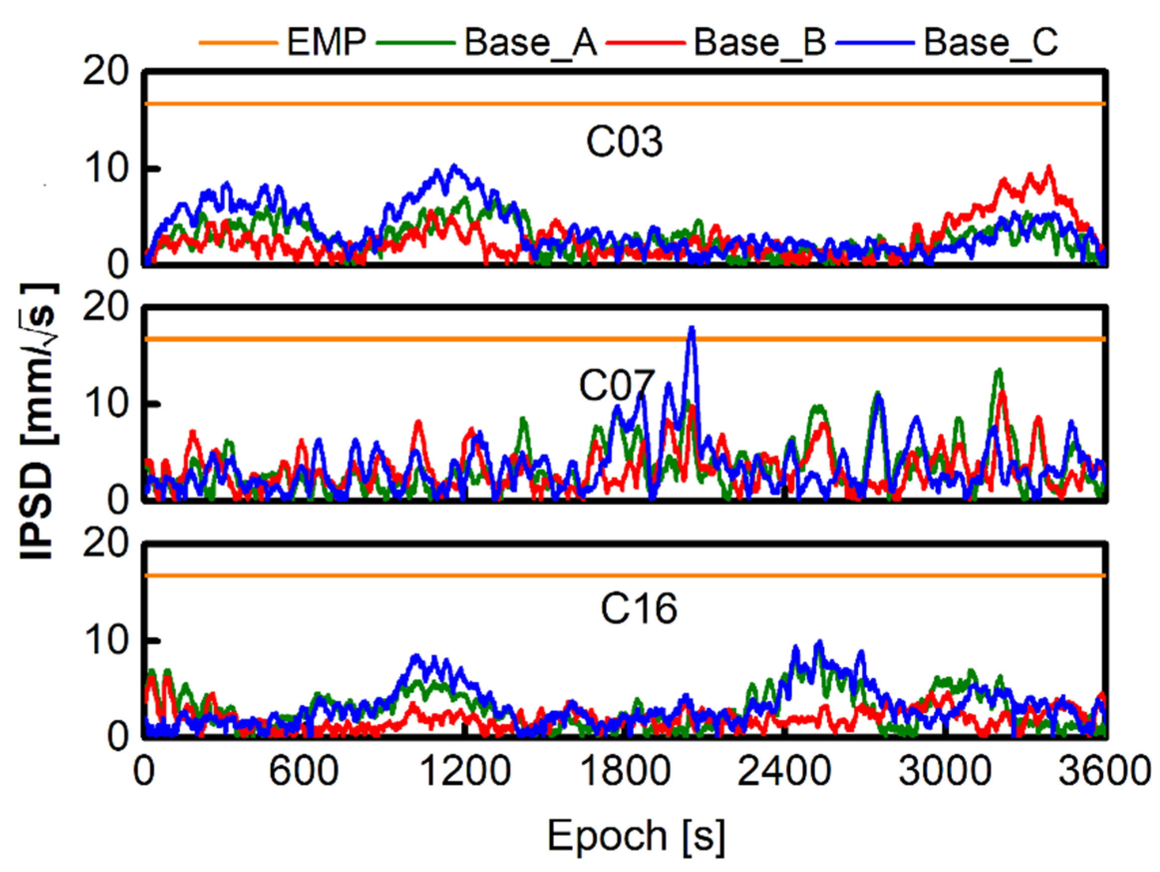
, and the larger the time interval, the smaller the impact level of noise. However, an excessively large difference interval will ignore ionospheric variations within the time interval, resulting in a decrease in the temporal resolution and not reflecting the rapid ionospheric variations. It is very important to determine the difference interval that can reflect the ionospheric variations [36]. For this reason, we study the ionospheric variance in unit time, and define statistics ( Δ I G F , m n s ( Δ t , i ) ) 2 / Δ t as referring to the ionospheric variance in unit time. If the cumulative variance value is a stable process, it shows that noise plays a major role. If the difference interval can reflect the ionospheric variations, the random walk of the ionosphere will change the slope of the curve. When the differential time interval is obtained, the IPSD can be calculated by Equation (44):
q 2 ( Δ ι r s , i ) = i = 1 i = n 1 ( Δ I G F , m n s ( Δ t , i ) ) 2 i = 1 i = n 2 ( Δ I G F , m n s ( Δ t , i ) ) 2 ( n 1 n 2 ) Δ t
Equation (44) represents the change in ionospheric variance within a certain time interval, that is, the change of PSD. When solving, we set the time span with the interval of n 1 n 2 = 60 s and calculate the PSD within this time period. Similarly, the calculation formula of TPSD can be obtained:
q 2 ( Δ τ , i ) = i = 1 i = n 1 ( Δ I F , m n s q ( Δ t , i ) ) 2 i = 1 i = n 2 ( Δ I F , m n s q ( Δ t , i ) ) 2 ( n 1 n 2 ) Δ t
When solving the PSD, the choice of differential time interval is very important. It can be seen from Equation (43) that with the increase of differential time interval, the influence of observation noise will become smaller and smaller, but too large a differential interval will also reduce the time resolution of the PSD. It is not conducive to real-time parameter constraints, so we will study the minimum differential time interval that can reflect atmospheric variations.

4. Experimental Validation

4.1. Experimental Data and Processing

The five reference stations identified as SHQA, HRSZ, MDTJ, JMTY, and HRFS in the CORS network were composed of four reference station networks, namely A, B, C, and D. The ambiguity fixing performance of the four reference station networks was studied. Among them, the reference station network C contained the user station “User”, which was used for testing the positioning performance of the user station under the correction of reference station error. The observation span was 28 April 2020, and the data sampling rate was 1 Hz. The distribution of reference stations and user stations is shown in Figure 3, and Table 2 provides baseline length and longitude and latitude information for the reference stations.
It can be seen from Table 2 that the distance between reference stations was more than 100 km, so the atmospheric error between reference stations could not be eliminated by observations difference [37] and had to be estimated as random walk parameters. By adjusting the PSD in the random walk, the ambiguity fixing performance can be significantly improved.
After determining the DD ambiguity of the reference station network using the LAMBDA method, the correctness of the DD ambiguity was first determined using the ratio value of the FFRatio test (Verhagen et al., 2013) [38]. At the same time, the correctness of the DD ambiguity at each frequency was determined using an ambiguity closure error of 0, satisfying the relationship:
Δ N j , A B + Δ N j , B C + Δ N j , C A = 0
While ensuring a fast ambiguity fixing time, it is also necessary to ensure a high ambiguity fixing success rate. Therefore, this study also analyzed statistics on the fixing success rate under atmospheric time-varying parameter constraints. The ambiguity fixing success rate was defined as the ratio of the epochs through the FFRatio test and the closure error test to the total epochs [39].

4.2. PSD Effect on Ambiguity Fixing Performance

In order to verify the influence of the PSD of the atmospheric parameters on the ambiguity fixing performance, the most commonly used empirical TPSD and IPSD, 1   c m / h and 1   m / h [19], were selected. Empirical values cannot be adjusted according to the actual atmospheric variations, so they are relatively loose. This will not cause distortion of the baseline due to the tight constraints during periods of severe atmospheric variations. We divided the data from four networks into 1 h periods to statistically analyze the ambiguity fixing time and ambiguity success rate of reference stations under different scaling factors. Figure 4 shows the ambiguity fixing time of the empirical IPSD 1   m / h at different scaling factors.
It can be seen from Figure 4 that the ambiguity fixing time at different times of IPSD was inconsistent, and the empirical IPSD was not optimal, which indicated that the empirical IPSD cannot optimize the ambiguity fixing time; optimal IPSD is at 1/4 of the empirical IPSD. At the same time, it was found that the fixing time on both sides of the optimal IPSD was not symmetrically distributed. The fixing time on the left side of the optimal IPSD (which means the IPSD is shrinking) sharply increased, because the IPSD was too small and the constraints of the ionospheric parameters were too tight. The fixing time on the right side of the optimal IPSD (indicating that the IPSD is increasing) was close to the optimal IPSD, so it is appropriate to give a loose constraint when accurate ionospheric prior information is not available. Figure 5 shows the ambiguity success rate of the empirical IPSD 1   m / h at different scaling factors.
Figure 5 shows that the ambiguity success rate was the same as the performance of the ambiguity fixing time. The IPSD of different times will affect the ambiguity success rate, which is not also symmetrically distributed on both sides of the optimal IPSD (1/4). On the left side of the optimal IPSD (which means the IPSD is shrinking), the success rate decreased rapidly, so the ionospheric constraints were too tight due to the too small IPSD, affecting the continuous ambiguity fixing of the reference station. Figure 6 shows the ambiguity fixing time of the empirical TPSD 1   c m / h at different scaling factors.
It can be seen from Figure 6 that the empirical TPSD was not optimal for ambiguity fixing time, and cannot play the most effective constraint. Unlike the impact of IPSD on the ambiguity fixing time, TPSD has a relatively small impact on the fixing time. This is because tropospheric variations are relatively gentle, and the changes in TPSD do not have a significant impact on the fixing time. Figure 7 shows the ambiguity success rate of the empirical TPSD 1   c m / h at different scaling factors.
As can be seen from Figure 7, consistent with the impact on the ambiguity fixing time, the best TPSD did not have the highest ambiguity success rate. The empirical TPSD cannot adjust according to the actual observation data, so a larger TPSD makes the ambiguity fixing performance of the reference station not optimal. It is necessary to establish a method to determine the TPSD associated with the actual observation data.

4.3. Real-Time Estimation Method for Atmospheric PSD

Since the empirical PSD cannot be adjusted according to the actual observation environment, a larger empirical value is selected, which also makes the empirical PSD unable to reach the maximum constraint performance, and is not optimal for the ambiguity fixing of the reference station. Therefore, the method for real-time estimation of PSD according to the observation data was studied. The baseline SHQA-JMTY (187KM) in Network A was taken as an example to study the IPSD and TPSD. Figure 8 shows the variation of ionospheric error and the cumulative variance ( Δ I G F , m n s ( Δ t , i ) / Δ t ) 2 under different difference intervals.
It can be clearly seen from Figure 8 that, when the difference interval was 1 s, the accumulation of variance showed the variation of white noise, which was a curve with relatively constant slope variation. When the time difference interval increased to 15 s, because the difference interval already reflected the ionospheric variation, the curve represented the variation of the ionosphere with time. When the time difference interval reached 30 s, the variation curve was already consistent with the 60 s variation curve, and increasing the difference interval had no significant effect on the separation of the ionosphere. Therefore, in this study, the 30 s difference interval was considered as an empirical difference interval that can reflect the ionospheric variations. Figure 9 shows the variation of the troposphere and the cumulative variance ( Δ I F , m n s q ( Δ t , i ) / Δ t ) 2 of different difference intervals of the C03 satellite.
It can also be clearly seen from Figure 9 that the tropospheric variation was relatively stable, and the variance curve at 1 s reflected the variation in white noise. Although the 10 min difference interval realized the variation in the atmosphere, it was quite different from the 20 min difference interval. Only when the difference interval reached 20 min was the variance variation in the atmosphere closer to the variance in the larger interval. Therefore, a 20 min difference interval was selected in the study as the empirical difference interval that can reflect the tropospheric variation.
According to the previous theoretical analysis, the slope of the variance curve in Figure 8 represents the square of the PSD. Equation (44) also gives the calculation equation of IPSD. It can be seen from the analysis in Figure 8 that the influence of observation noise will not be significant when the difference interval reaches 30 s, so the variance curve of 30 s difference interval was selected when estimating the IPSD. At the same time, the updated IPSD was obtained continuously with a sliding window of 1 min. The IPSD variation curve for C03, C07, and C16 is shown in Figure 10.
The IPSD of each satellite in Figure 10 showed a trend of continuous variation over time, and the IPSD of the C16 satellite varied slowly, which corresponded to the smooth variation of the ionospheric error of C16 satellite in Figure 8. In the analysis of Figure 9, the effect of observation noise was not significant when the difference time interval was 20 min. The tropospheric variance variation curve with the difference interval of 20 min was selected, and the updated TPSD was obtained continuously with the sliding window of 1 min. Equation (45) also gives the calculation equation of TPSD. Figure 11 shows the time series of the TPSD.
From Figure 11, it can be seen that the TPSD values were significantly smaller than those for the IPSD, and the trend of variation was also relatively stable, which is caused by the slow variation in tropospheric errors.

4.4. Fixing Performance Analysis between Estimated PSD and Empirical PSD

The estimated PSD can provide more reasonable constraints on the atmospheric parameters and improve the ambiguity fixing performance. Through the research in Section 4.3, the PSD can be estimated according to the actual observation data. To compare the ambiguity fixing performance of the estimated PSD with the empirical PSD, the following PSD schemes were set to solve the ambiguity.
Scheme 1: Estimated PSD (EST).
Scheme 2: Empirical PSD (EMP), TPSD: 1   c m / h ; IPSD: 1   m / h [19].
Divide the data of the four networks into 1 h periods for statistical analysis of the ambiguity fixing time and ambiguity fixing success rate. Figure 12 and Figure 13 show the statistics for the ambiguity fixing time and the ambiguity fixing success rate between estimated PSD and empirical PSD.
From Figure 12, it can be seen that for the ambiguity fixing time of the reference network, EST PSD was always better than EMP PSD. Among the four networks, EST PSD improved the fixing time by 14.7%, 19.3%, 17.9%, and 21.5%. This is because the empirical EMP cannot be adjusted based on the actual observations situation, and can only choose relatively loose constraint values, with limited constraint effects. The ambiguity fixing success rate of EST PSD in Figure 13 was significantly improved, by 9.5%, 12.9%, 12.7%, and 11.9% in the four networks. Figure 14 shows the sequence of ambiguity floating solutions between estimated PSD and empirical PSD.
From Figure 14, it can be seen that there were differences in the early stage of the convergence process of the ambiguity floating solutions, which is also the main reason for the inconsistent ambiguity fixing time. In the later stage of the convergence, the floating solutions difference between the two methods will continue to decrease. Figure 15 shows the estimated IPSD and empirical IPSD for Network A over a period of time.
From Figure 15, it can be seen that EMP IPSD was much larger than EST IPSD, and EMP IPSD always maintained a value that cannot be adjusted in real time based on ionospheric variation. However, EST IPSD showed constant variation and showed different trends on different satellites, which corresponded to the ionospheric variation. EST IPSD variation on each baseline was similar, which was due to the consistency of ionospheric variation in small areas. Figure 16 shows the comparison of estimated TPSD and empirical TPSD.
It can be seen from Figure 16 that the TPSD values were much smaller than those of the IPSD. The overall variation of the troposphere is stable, and the variation of TPSD is relatively stable. The estimated TPSD is also smaller than the empirical TPSD. Estimated TPSD will impose stronger constraints on the equation, and this constraint will not cause divergence of the positioning results.

4.5. User Observations Error Elimination and Positioning

Unlike general NRTK based on DD error correction, the undifferenced NRTK based on undifferenced error correction values in this paper does not directly generate error correction information after the DD ambiguity. Instead, UD ambiguity conversion is performed on the basis of DD ambiguity fixing, and error correction information is independently generated through the original observations of each reference station. Overcoming the correlation of error correction values between reference stations, the positioning is not limited by the number of reference stations and can flexibly select reference stations that need to broadcast error correction values. At the same time, except for the ambiguity parameter, the meaning of all errors is consistent with the original observation, retaining the characteristics of errors on the reference station. Figure 17 shows the error correction values of the UD ionosphere and troposphere generated by the three reference stations.
From Figure 17, it can be seen that, compared to the traditional NRTK, the undifferenced NRTK in this paper can independently generate error correction values for each reference station, and the correction values for each station are independent of each other. The variation trend of the ionosphere at each station is similar, and there is also consistency among satellites. The troposphere also exhibits similar patterns at various stations. The error correction value generated on each reference station are used to generate a comprehensive error correction value through an error interpolation model to correct the errors of each satellite on the user. Figure 18 shows the variation in atmospheric residual errors on each satellite after correction by the reference station error.
From Figure 18, it can be seen that the variation in residual ionospheric error is relatively stable, and the error always maintains a small value. At the same time, there is also a trend of variation over time, which is caused by the variation in residual ionospheric error after error correction. The fluctuation of tropospheric errors is often large due to the presence of receiver clock errors. The consistent trend of error changes among the three satellites also indicates that this fluctuation trend is caused by receiver errors, so it can be concluded that the variation in residual tropospheric errors is also very stable, After correction, the residuals of each satellite are relatively small. Figure 19 shows the user positioning results for the user in Network C.
As can be seen from Figure 19, except for individual points, the positioning accuracy in the plane direction is always kept within 0.1 m, and the positioning accuracy in the U direction can also reach the centimeter level, which can meet the needs of real-time dynamic positioning.

5. Conclusions

This paper provides a detailed introduction to an undifferenced NRTK positioning model considering the constraints of time-varying atmospheric characteristics. Starting from the UD observation equation, the generation of error correction information for single reference stations and multiple reference stations, interpolation of error correction information, and user error correction and positioning are introduced in detail. In undifferenced NRTK, the ambiguity fixing of the reference station is the starting point for generating high-precision error correction information and high-precision positioning. Therefore, this paper studied the time-varying characteristics of atmospheric parameters for the ambiguity fixing of the reference station. The atmospheric delay error separated from the original observations contains a large amount of observation noise, which affects the determination of the atmospheric error PSD. This paper reduced the impact of observation noise by increasing the difference interval. The estimated PSD was used to constrain the atmospheric parameters in the ambiguity fixing. Compared with the empirical PSD, the estimated PSD in this paper improved the ambiguity fixing time by an average of 18.4%, and increased by 11.7% the ambiguity fixing success rate. The performance of the reference station ambiguity fixing was far better than with the empirical PSD method. Finally, the user error was corrected through the UD atmospheric error generated after the ambiguity fixing of the reference station, and user high-precision real-time dynamic positioning was achieved.

Author Contributions

J.L. conceived the idea and designed the experiments with H.Z., Y.L., M.Z. and A.X.; J.L. also wrote the main manuscript. H.Z., Y.L., M.Z. and A.X. reviewed the paper. All components of this research were carried out under the supervision of H.Z and A.X. All authors have read and agreed to the published version of the manuscript.

Funding

This research was funded by the National Natural Science Foundation of China (Nos. 42030109, 42074012) and the open fund of the State Key Laboratory of Satellite Navigation System and Equipment Technology (No. CEPNT-2018KF-13), and it was supported by the LiaoNing Revitalization Talents Program (Nos. XLYC2002101, XLYC2008034, XLYC2002098).

Data Availability Statement

The authors gratefully acknowledge the Heilongjiang CORS network for providing the multi-GNSS data. The other datasets are available from the corresponding author on reasonable request.

Acknowledgments

The authors gratefully acknowledge the Heilongjiang CORS network for providing the multi-GNSS data.

Conflicts of Interest

The authors declare no conflict of interest.

References

  1. Yang, Y.; Ding, Q.; Gao, W.; Li, J.; Xu, Y.; Sun, B. Principle and Performance of BDSBAS and PPP-B2b of BDS-3. Satell. Navig. 2022, 3, 5. [Google Scholar] [CrossRef]
  2. Li, P.; Zhang, X. Integrating GPS and GLONASS to Accelerate Convergence and Initialization Times of Precise Point Positioning. Gps Solut. 2014, 18, 461–471. [Google Scholar] [CrossRef]
  3. Teunissen, P.J.G. The Ionosphere-Weighted GPS Baseline Precision in Canonical Form. J. Geod. 1998, 72, 107–111. [Google Scholar] [CrossRef]
  4. Odijk, D.; Van Der Marel, H.; Song, I. Precise GPS Positioning by Applying Ionospheric Corrections from an Active Control Network. Gps Solut. 2000, 3, 49–57. [Google Scholar] [CrossRef]
  5. Wübbena, G.; Schmitz, M.; Bagge, A. PPP-RTK: Precise Point Positioning Using State-Space Representation in RTK Networks. In Proceedings of the ION GNSS 2005, Long Beach, CA, USA, 13–16 September 2005; pp. 2584–2594. [Google Scholar]
  6. Chen, D.; Ye, S.; Xu, C.; Jiang, W.; Jiang, P.; Chen, H. Undifferenced Zenith Tropospheric Modeling and Its Application in Fast Ambiguity Recovery for Long-Range Network RTK Reference Stations. GPS Solut. 2019, 23, 26. [Google Scholar] [CrossRef]
  7. Geng, J.; Bock, Y. GLONASS Fractional-Cycle Bias Estimation across Inhomogeneous Receivers for PPP Ambiguity Resolution. J. Geod. 2016, 90, 379–396. [Google Scholar] [CrossRef]
  8. Rui, T.; Zhang, H.; Ge, M.; Huang, G. A Real-Time Ionospheric Model Based on GNSS Precise Point Positioning. Adv. Space Res. 2013, 52, 1125–1134. [Google Scholar]
  9. Teunissen, P.J.G. The Geometry-Free GPS Ambiguity Search Space with a Weighted Ionosphere. J. Geod. 1997, 71, 370–383. [Google Scholar] [CrossRef]
  10. Paziewski, J. Study on Desirable Ionospheric Corrections Accuracy for Network-RTK Positioning and Its Impact on Time-to-Fix and Probability of Successful Single-Epoch Ambiguity Resolution. Adv. Space Res. 2016, 57, 1098–1111. [Google Scholar] [CrossRef]
  11. Li, Z.; Yuan, Y.; Wang, N.; Hernandez-Pajares, M.; Huo, X. SHPTS: Towards a New Method for Generating Precise Global Ionospheric TEC Map Based on Spherical Harmonic and Generalized Trigonometric Series Functions. J. Geod. 2015, 89, 331–345. [Google Scholar] [CrossRef]
  12. Olivares-Pulido, G.; Terkildsen, M.; Arsov, K.; Teunissen, P.J.G.; Khodabandeh, A.; Janssen, V. A 4D Tomographic Ionospheric Model to Support PPP-RTK. J. Geod. 2019, 93, 1673–1683. [Google Scholar] [CrossRef]
  13. Odijk, D. Weighting Ionospheric Corrections to Improve Fast GPS Positioning Over Medium Distances. In Proceedings of the ION GPS 2000, Salt Lake City, UT, USA, 19–22 September 2000; pp. 1113–1123. [Google Scholar]
  14. Liu, G.C.; Lachapelle, G. Ionosphere Weighted GPS Cycle Ambiguity Resolution1. In Proceedings of the ION NTM 2002, Institute of Navigation, San Diego, CA, USA, 28–30 January 2002; pp. 889–899. [Google Scholar]
  15. Wielgosz, P. Quality Assessment of GPS Rapid Static Positioning with Weighted Ionospheric Parameters in Generalized Least Squares. Gps Solut. 2011, 15, 89–99. [Google Scholar] [CrossRef]
  16. Bock, Y. Medium Distance GPS Measurements. In GPS for Geodesy; Springer: Berlin/Heidelberg, Germany, 2008. [Google Scholar]
  17. Goad, C.C.; Ming, Y. A New Approach to Precision Airborne GPS Positioning for Photogrammetry. Photogramm. Eng. Remote Sens. 1997, 63, 1067–1077. [Google Scholar]
  18. Borko, A.; Even-Tzur, G. Stochastic Model Reliability in GNSS Baseline Solution. J. Geod. 2021, 95, 20. [Google Scholar] [CrossRef]
  19. Tang, W.; Liu, W.; Zou, X.; Li, Z.; Chen, L.; Deng, C.; Shi, C. Improved Ambiguity Resolution for URTK with Dynamic Atmosphere Constraints. J. Geod. 2016, 90, 1359–1369. [Google Scholar] [CrossRef]
  20. Schaer, S.; Beutler, G.; Rothacher, M.; Brockmann, E.; Wild, U. The Impact of the Atmosphere and Other Systematic Errors on Permanent GPS Networks; Springer: Berlin/Heidelberg, Germany, 2000. [Google Scholar]
  21. Odijk, D.; Zhang, B.; Khodabandeh, A.; Odolinski, R.; Teunissen, P.J.G. On the Estimability of Parameters in Undifferenced, Uncombined GNSS Network and PPP-RTK User Models by Means of S-system Theory. J. Geod. 2016, 90, 15–44. [Google Scholar] [CrossRef]
  22. Ouassou, M.; Jensen, A.; Gjevestad, J.; Kristiansen, O. Next Generation Network Real-Time Kinematic Interpolation Segment to Improve the User Accuracy. Int. J. Navig. Obs. 2015, 2015, 346498. [Google Scholar] [CrossRef]
  23. Dai, L.; Han, S.; Wang, J.; Rizos, C. Comparison of Interpolation Algorithms in Network-Based GPS Techniques. Navigation 2003, 50, 277–293. [Google Scholar] [CrossRef]
  24. Alber, C.; Ware, R.; Rocken, C.; Braun, J. Obtaining Single Path Phase Delays from GPS Double Differences. Geophys. Res. Lett. 2000, 27, 2661–2664. [Google Scholar] [CrossRef]
  25. Zhang, J.; Lachapelle, G. Precise Estimation of Residual Tropospheric Delays Using a Regional GPS Network for Real-Time Kinematic Applications. J. Geod. 2001, 75, 255–266. [Google Scholar] [CrossRef]
  26. Boehm, J.; Niell, A.; Tregoning, P.; Schuh, H. Global Mapping Function (GMF): A New Empirical Mapping Function Based on Numerical Weather Model Data. Geophys. Res. Lett. 2006, 33, L07304. [Google Scholar] [CrossRef]
  27. Saastamoinen, J. Atmospheric Correction for the Troposphere and Stratosphere in Radio Ranging Satellites. In The Use of Artificial Satellites for Geodesy; American Geophysical Union: Washington, DC, USA, 1971. [Google Scholar] [CrossRef]
  28. Zhong, P.; Ding, X.; Yuan, L.; Xu, Y.; Kwok, K.; Chen, Y. Sidereal Filtering Based on Single Differences for Mitigating GPS Multipath Effects on Short Baselines. J. Geod. 2010, 84, 145–158. [Google Scholar] [CrossRef]
  29. Li, J.; Zhu, H.; Xu, A.; Xu, Z. Estimating Ionospheric Power Spectral Density for Long-Range RTK Positioning Using Uncombined Observations. GPS Solut. 2023, 27, 109. [Google Scholar] [CrossRef]
  30. Xuan, Z.; Wang, Y.; Deng, C.; Tang, W.; Shi, C. Instantaneous BDS + GPS Undifferenced NRTK Positioning with Dynamic Atmospheric Constraints. GPS Solut. 2018, 22, 17. [Google Scholar]
  31. Teunissen, P.J.G. Influence of Ambiguity Precision on the Success Rate of GNSS Integer Ambiguity Bootstrapping. J. Geod. 2007, 81, 351–358. [Google Scholar] [CrossRef]
  32. Ge, M.; Gendt, G.; Dick, G.; Zhang, F.P.; Rothacher, M. A New Data Processing Strategy for Huge GNSS Global Networks. J. Geod. 2006, 80, 199–203. [Google Scholar] [CrossRef]
  33. Deng, C.; Tang, W.; Liu, J.; Shi, C. Reliable Single-Epoch Ambiguity Resolution for Short Baselines Using Combined GPS/BeiDou System. GPS Solut. 2014, 18, 375–386. [Google Scholar] [CrossRef]
  34. Li, Z.; Chen, W.; Ruan, R.; Liu, X. Evaluation of PPP-RTK Based on BDS-3/BDS-2/GPS Observations: A Case Study in Europe. GPS Solut. 2020, 24, 38. [Google Scholar] [CrossRef]
  35. Teunnissen, P.J.G. The Least-Squares Ambiguity Decorrelation Adjustment: A Method for Fast GPS Integer Ambiguity Estimation. J. Geod. 1995, 70, 65–82. [Google Scholar] [CrossRef]
  36. Zhu, H.; Li, J.; Tang, L.; Ge, M.; Xu, A. Improving the Stochastic Model of Ionospheric Delays for BDS Long-Range Real-Time Kinematic Positioning. Remote Sens. 2021, 13, 2739. [Google Scholar] [CrossRef]
  37. Chen, L.; Zheng, F.; Gong, X.; Jiang, X. GNSS High-Precision Augmentation for Autonomous Vehicles: Requirements, Solution, and Technical Challenges. Remote Sens. 2023, 15, 1623. [Google Scholar] [CrossRef]
  38. Verhagen, S.; Li, B.; Teunissen, P. Ps-LAMBDA: Ambiguity Success Rate Evaluation Software for Interferometric Applications. Comput. Geosci. 2013, 54, 361–376. [Google Scholar] [CrossRef]
  39. Zhang, B.; Ke, C.; Zha, J.; Hou, P.; Liu, T.; Yuan, Y.; Li, Z. Undifferenced and Uncombined PPP-RTK:Algorithmic Models, Prototype Terminals and Field-Test Results. Acta Geod. Cartogr. Sin. 2022, 51, 1725. [Google Scholar]
Figure 1. Undifferenced integer ambiguity conversion process.
Remotesensing 15 04784 g001
Figure 2. Schematic representation of the regional error interpolation.
Remotesensing 15 04784 g002
Figure 3. Distribution of GNSS stations.
Remotesensing 15 04784 g003
Figure 4. Ambiguity fixing time with different IPSDs expressed by the scale factor applied to the empirical IPSD (the value of horizontal axis represents n in the scaled multiple of 2 n ).
Remotesensing 15 04784 g004
Figure 5. Ambiguity success rate with different IPSDs expressed by the scale factor applied to the empirical IPSD (the value of horizontal axis represents n in the scaled multiple of 2 n ).
Remotesensing 15 04784 g005
Figure 6. Ambiguity fixing time with different TPSDs expressed by the scale factor applied to the empirical TPSD (the value of horizontal axis represents n in the scaled multiple of 2 n ).
Remotesensing 15 04784 g006
Figure 7. Ambiguity success rate with different TPSDs expressed by the scale factor applied to the empirical TPSD (the value of horizontal axis represents n in the scaled multiple of 2 n ).
Remotesensing 15 04784 g007
Figure 8. Ionospheric variation and cumulative variance under different difference intervals.
Remotesensing 15 04784 g008
Figure 9. Tropospheric variation and cumulative variance under different difference intervals.
Remotesensing 15 04784 g009
Figure 10. Time series of the IPSD for C03, C07, and C16.
Remotesensing 15 04784 g010
Figure 11. Time series of the TPSD for C03.
Remotesensing 15 04784 g011
Figure 12. Ambiguity fixing time between estimated PSD and empirical PSD.
Remotesensing 15 04784 g012
Figure 13. Ambiguity fixing success rate between estimated PSD and empirical PSD.
Remotesensing 15 04784 g013
Figure 14. Ambiguity floating solutions between estimated PSD and empirical PSD.
Remotesensing 15 04784 g014
Figure 15. A comparison plot of the estimated IPSD with the empirical IPSD.
Remotesensing 15 04784 g015
Figure 16. A comparison plot of the estimated TPSD with the empirical TPSD.
Remotesensing 15 04784 g016
Figure 17. Sequence of UD ionosphere and troposphere error-correction values.
Remotesensing 15 04784 g017
Figure 18. The user residual series after the error correction.
Remotesensing 15 04784 g018
Figure 19. User positioning error sequence.
Remotesensing 15 04784 g019
Table 1. Reference station OSR correction information and the error correction process of the user station.
TypeReceiver ErrorsSatellite ErrorsAtmospheric Errors
Single reference station d t A δ A , j d t s δ j s T A s ι A s
Multiple reference stations α A d t A + α B d t B + α C d t C
α A δ A , j + α B δ B , j + α C δ C , j
d t s δ j s α A T A s + α B T B s + α C T C s
α A ι A , j s + α B ι B , j s + α C ι C , j s
User station d t r δ r , j d t s δ j s T r s ι r s
Table 2. Information on baselines employed in the experimental validation.
BaselineLength/KMLocation
SHQA-JMTY (187 KM)187(46:52N,127:28E), (46:47N,129:56E)
JMTY-HRFS (121 KM)121(46:47N,129:56E), (46:15N,128:33E)
HRFS-SHQA (107 KM)107(46:15N,128:33E), (46:52N,127:28E)
JMTY-MDTJ (171 KM)171(46:47N,129:56E), (45:16N,130:14E)
MDTJ-HRFS (170 KM)170(45:16N,130:14E), (46:15N,128:33E)
MDTJ-HRSZ (178 KM)178(45:16N,130:14E), (45:12N, 127:58E)
HRSZ-HRFS (125 KM)125(45:12N,127:58E), (46:15N,128:33E)
HRSZ-SHQA (189 KM)189(45:12N,127:58E), (46:52N,127:28E)
Disclaimer/Publisher’s Note: The statements, opinions and data contained in all publications are solely those of the individual author(s) and contributor(s) and not of MDPI and/or the editor(s). MDPI and/or the editor(s) disclaim responsibility for any injury to people or property resulting from any ideas, methods, instructions or products referred to in the content.

