Global Satellite Monitoring of Exothermic Industrial Activity via Infrared Emissions

Abstract

This paper reports on the first daily global monitoring program for natural gas flaring and industrial sites producing waste heat based on satellite observed infrared emissions. The Visible Infrared Imaging Radiometer Suite (VIIRS) collects nightly global infrared data in spectral bands ranging from near infrared (NIR) to longwave infrared (LWIR), providing a unique capability to detect and characterize infrared emitters at night. The VIIRS nightfire (VNF) algorithm identifies infrared (IR) emitters with multiple spectral bands and calculates the temperature, source area, and radiant heat via Planck curve fitting and physical laws. VNF data are produced nightly and extend from 2012 to the present. The most common infrared emitter is biomass burning, which must be filtered out. Industrial IR emitters can be distinguished from biomass burning based on temperature and persistence. The initial filtering to remove biomass burning was performed with 15 arc second grids formed from eleven years of VIIRS data, spanning 2012–2022. The locations and shapes of the remaining features were used to guide the generation of super-resolution pixel center clouds. These data clouds were then analyzed to define bounding vectors for single emitters and to split larger clusters into multiple emitters. A total of nearly 20,000 IR emitters were identified; each was assigned an identification number, and the type of emitter was recorded. Nightly temporal profiles were produced for each site, revealing activity patterns back to 2012. Nightly temporal profiles were kept current with weekly updates. Temporal profiles from individual sites were aggregated by country to form monthly profiles extending back to 2012. The nightly and monthly temporal profiles were suitable for analyzing industrial production, identifying disruption events, and tracking recovery. The data could also be used in tracking progress in energy conservation and greenhouse gas emission inventories.

1. Introduction

Long-term satellite monitoring of human activities has become an increasingly valuable way to record human activities and estimate variables that are difficult to measure in situ, such as population, economic activity, power, and fuel consumption. Ongoing satellite monitoring includes a wide range of phenomena, from tracking the growth of built infrastructure, emissions of greenhouse gases and pollutants, and radiant emissions from electric lighting, radio and microwave, and exothermic (heat-producing) industrial activities. The specific details of built infrastructure are best observed with near-meter-scale daytime multispectral imagery [1] and synthetic aperture radar imagery [2]. Other satellite sensors focus on pollution sources, such as the Greenhouse Gas Satellite (GHGSat) [3], NASA’s Earth Surface Mineral Dust Source Investigation (EMIT) [4], the planned Carbon Mapper [5], and others. For many decades, intelligence agencies have collected and analyzed signals collected from satellite sensors in radio frequencies (RF), with the primary interest being the recording of wireless communications. Those data are highly classified and inaccessible for science applications. More recently, Hawkeye 360 began commercial services for unclassified collection of radio frequency signals from space [6].

Global mapping of electric lighting from satellites requires nighttime observations in the visible wavelength range with sensors having low-light imaging capabilities. The visible band detection limits for sensors designed for the daytime imaging of reflected sunlight are not low enough for the detection of the carpet of lighting present on the Earth’s surface. Currently, two polar orbiting meteorological sensor series operate with specialized light-intensified panchromatic spectral bands straddling the visible and near infrared (VNIR), providing data suitable for global mapping of nighttime lights. This includes the U.S. Air Force Defense Meteorological Satellite Program (DMSP) Operational Linescan System (OLS) and the NASA/NOAA Visible Infrared Imaging Radiometer Suite (VIIRS). These sources are used to produce the global time series of satellite observed nighttime lights, which now span three decades back to 1992 [7].

The infrared is the obvious place to look for exothermic industrial activities in Earth observation satellite data. However, the detection of these sources has to contend with reflected sunlight during the day in the visible to midwave infrared (0.4 to 5 µm), background radiant emissions in the mid-to-longwave infrared (3 to 12 µm), plus co-mingling with radiances from electric lighting at night. In this paper we describe the assembly of long-term records of exothermic industrial activity derived from nighttime VIIRS data, taking advantage of four daytime channels that continue to collect at night. The band centers and spatial resolutions for the key infrared bands used in our study are listed in

Table 1. Moderate-resolution VIIRS spectral bands collecting at night.

Band Designation	Central Wavelength (Micrometers, µm)	Nadir Footprint (Meters)	Edge-of-Scan Footprint (Meters)
DNB	0.7	742 × 742	742 × 742
M7	0.885	742 × 776	1600 × 1558
M8	1.24	742 × 776	1600 × 1558
M10	1.61	742 × 776	1600 × 1558
M11	2.25	742 × 776	1600 × 1558
M12	3.7	742 × 776	1600 × 1558
M13	4.05	742 × 776	1600 × 1558
M14	10.763	742 × 776	1600 × 1558
M15	11.45	742 × 776	1600 × 1558
M16	12.013	742 × 776	1600 × 1558

.

Moderate spatial resolution (~1 km²) polar orbiting meteorological satellite sensors, such as VIIRS, are primarily designed for the observation of the large-scale processes within the atmosphere and Earth’s surface: clouds, the cryosphere, photosynthetic organisms, and land and ocean surfaces. Typically, these features are vast in extent and can readily fill entire VIIRS pixel footprints. The VIIRS detection limits, saturation radiance, and quantization levels across the visible to shortwave infrared are set based on solar reflectance levels spanning low- to high-albedo surfaces. The exception to this is the low-light imaging day/night band (DNB), which features a million-fold amplification of signal to enable the detection of moonlit clouds [8].

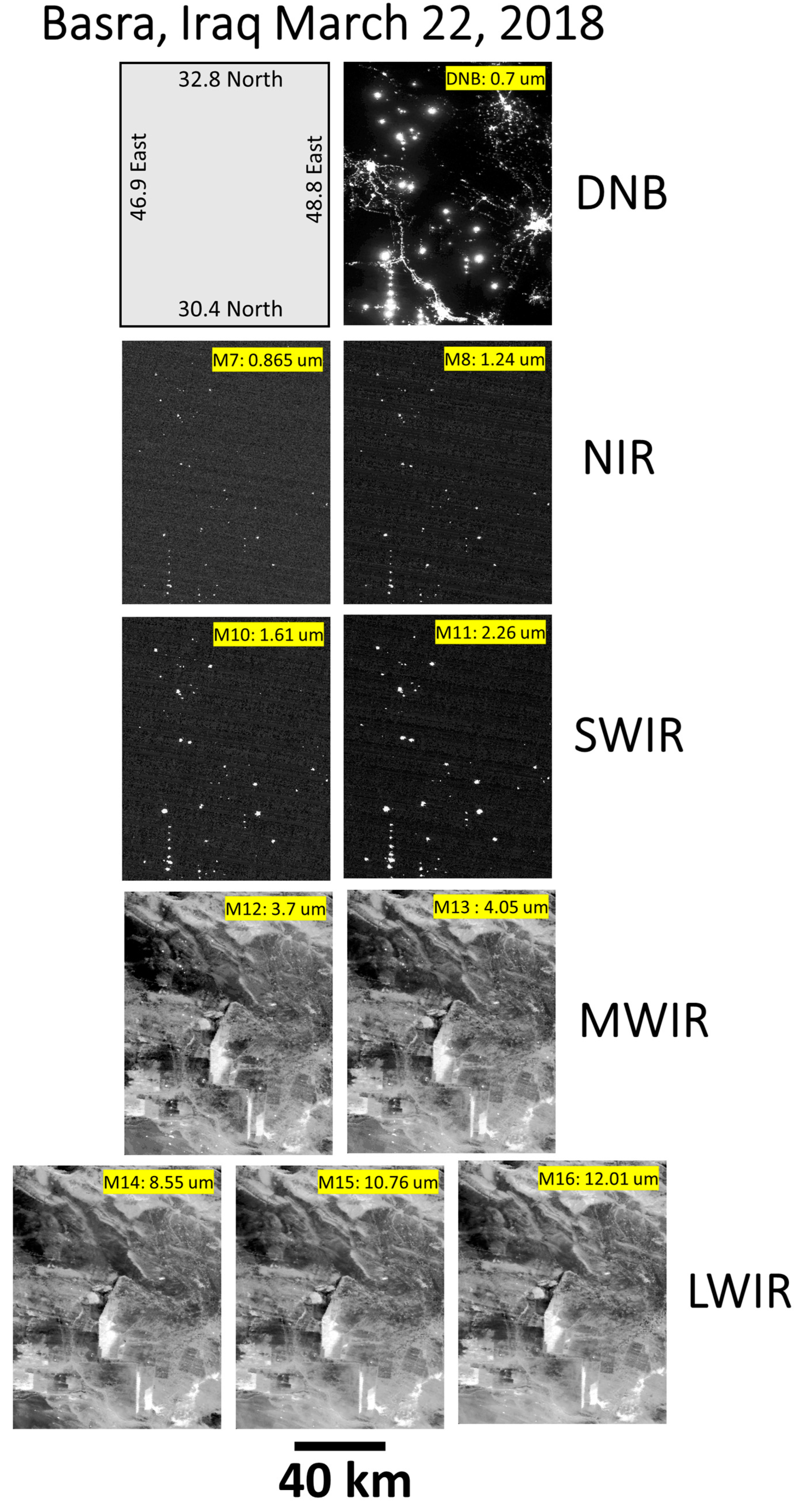
VIIRS is unique in its nightly, global collection of spectral channels designed for daytime imaging in two near-infrared (NIR) and two shortwave infrared (SWIR) bands. Specifically, these are the moderate spatial resolution bands designated as M7, M8, M10, and M11, collectively referred to as M7–11. With sunlight eliminated, industrial infrared emitters readily stand out from the sensor’s noise floor in the nighttime data collected by M7–11 (Figure 1). The radiances from electric lighting and exothermic industrial emitters both contribute to the VIIRS DNB (Figure 1). However, the detection limits for M7–11 are not low enough to detect electric lighting, except for a handful of sites worldwide.

In 2012, EOG developed the VIIRS nightfire (VNF) algorithm [9] to exploit the detection of Earth surface infrared emitters in M7–11. VNF assumes the M7–11 detection radiances are entirely attributable to subpixel infrared emitters, with no contribution from electric lighting and no contribution from the background. Dual Planck curve fitting is performed to define the Planck curves for the emitter and the background using the radiances from band M7 through M16. This effectively unmixes the emitter and background radiance in the midwave infrared. For more than a decade, EOG has used VNF to detect and monitor gas flaring worldwide [10]. The hot emitter Planck curve is used to calculate the temperature, source size, and radiant heat using physical laws.

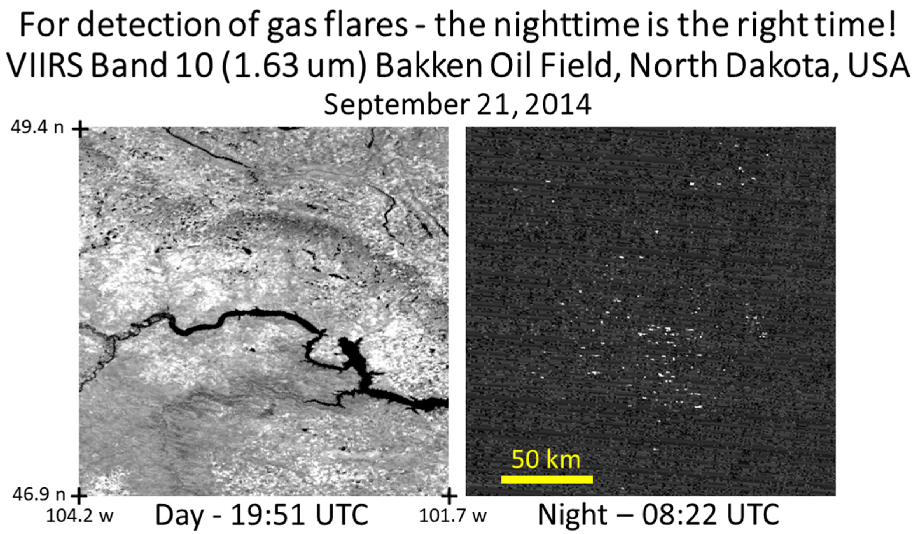
Since flares can burn day or night, one could ask why nighttime VIIRS data are widely used in detecting and monitoring gas flaring. The answer is that the peak radiant emissions from flares are in the shortwave infrared, and the flares are miniscule compared with the VIIRS pixel footprints. Flares cannot be readily detected in the daytime VIIRS SWIR band data due to the preponderance of reflected sunlight (Figure 2) and coarse spatial resolution. It should be noted that flares are detectable in the SWIR with 30 m spatial resolution daytime Landsat [11,12] and daytime data collected by ESA’s Sentinel 2 sensors [13], direct analogs to Landsat.

The Earth Observation Group developed procedures to identify flaring sites using either years or multiple years of VNF data [10]. The primary emitter type detected by VNF is biomass burning, which has a lower temperature than flaring. To filter out biomass burning, EOG screens out VNF detections for sites whose average temperatures are below 1300 K. Flares typically burn in the range of 1600 to 2000 K, while biomass burning temperatures are about half of that. The 1300 K threshold, combined with a one percent detection frequency threshold, works quite well to eliminate most biomass burning, making it possible to identify flaring sites and to estimate their flared gas volume through time without confusion with biomass burning VNF detections. But what is lost in this filtering are the radiant emissions from non-flaring industrial sites that are at temperatures lower than 1300 K.

In this study we removed the 1300 K threshold and implemented new methods to filter out biomass burning to identify non-flaring exothermic industrial sites. We were not the first group to do this with VNF data. Lui et al. [14] constructed a global map of 15,199 industrial infrared emitters from four years of VNF data. Other investigators have assembled regional maps of infrared emitters using either VNF or midwave infrared hotspot detections [15,16,17]. In this paper we present results from a new inventory of industrial IR emitters worldwide based on the nightly record of VNF detections from 2012 through 2022.

The primary objectives of this study were to (1) implement a nightly global monitoring system for heat-producing industrial sites worldwide, (2) label the sites by industry types, and (3) produce and keep updated long-term temporal profiles of the site temperature and heat output as observed from space.

2. VIIRS Nightfire

In 2012, EOG introduced the VIIRS Nightfire algorithm (VNF) [9] for the detection and characterization of subpixel IR emitters at night with a combination of near-infrared (NIR), shortwave infrared (SWIR), and midwave infrared (MWIR) radiances collected by VIIRS. Currently, VNF data are produced worldwide on a nightly basis with VIIRS data collected from the Suomi NPP and NOAA-20 satellites. VNF runs in near-real time, making it possible to provide alerts for detections found in specific areas of interest, such as volcanoes or national parks. The nightly VNF archive extends back to 2012 and is accessible through https://eogdata.mines.edu/products/vnf/ (accessed on 1March 2023).

VNF has five independent detectors to identify pixels containing IR emitters. These algorithms are run on NOAA-produced Science Data Records (SDRs) prior to geolocation. Thus, only the pixels with detections are geolocated, streamlining the processing of 150 gigabytes of nighttime data collected by each VIIRS instrument per night.

The first four detectors operate on the two NIR and two SWIR bands (M7–11) and function by setting the detection thresholds at the mean plus four standard deviations calculated on each of the one-minute granules provided by NOAA. Each granule spans 3000 km wide on the Earth’s surface and contains approximately two million pixels. At night, the VIIRS NIR and SWIR images primarily record the noise floor of the sensor. Because IR emitters are so rare, they can easily be detected with this simple algorithm. The NIR and SWIR detections are particularly valuable to VNF because the radiance can be fully attributed to the emitters present in the pixel footprint.

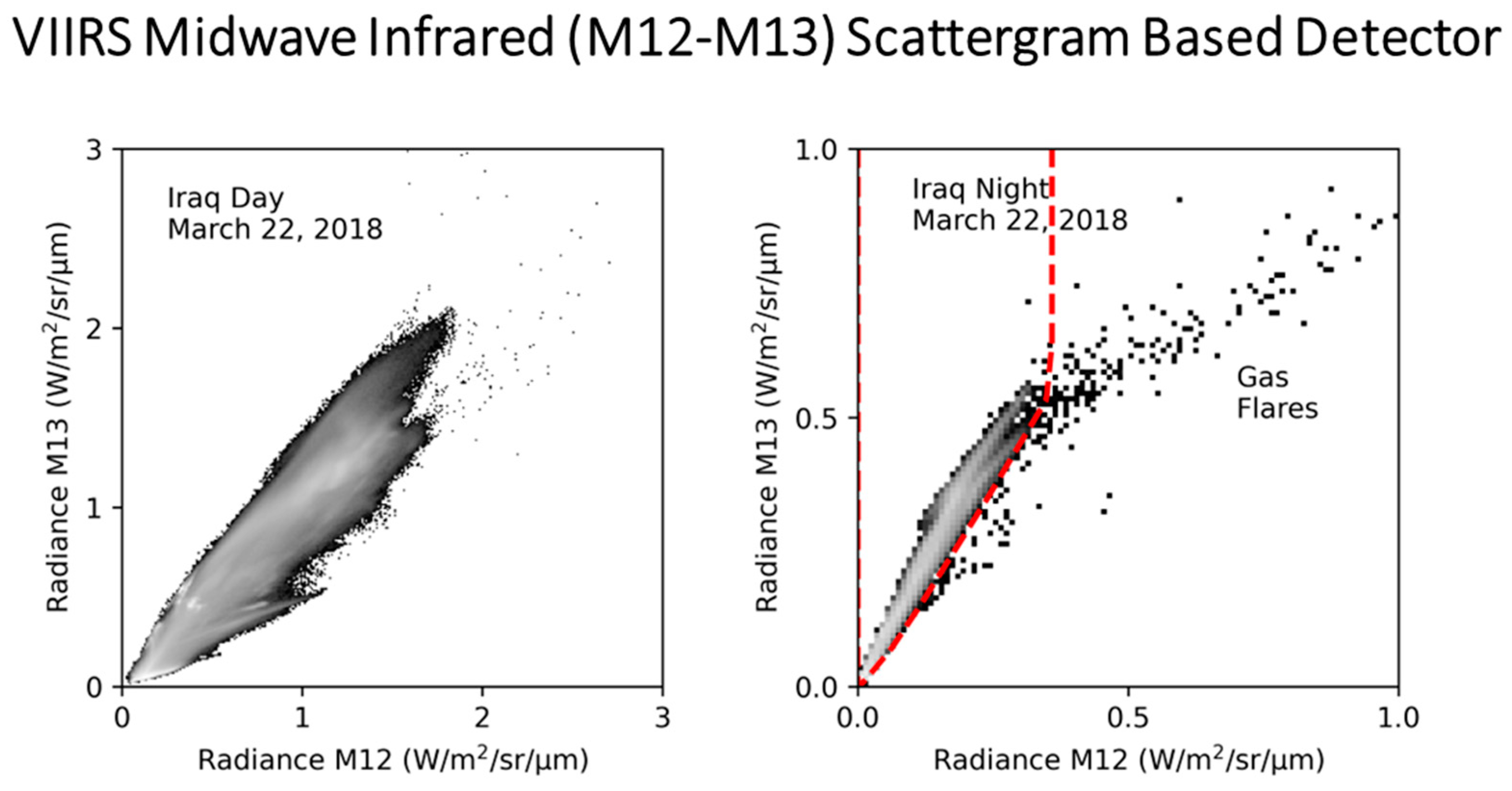
VNF’s fire detection algorithm operates on the MWIR channels and is more complicated due to the presence of radiant emissions from background objects such as clouds, water bodies, and land surfaces (Figure 3). Because the two MWIR spectral bands are so close spectrally (3.7 vs. 4.05 µm), at night, pure background pixels align to form a tight diagonal baseline on a M12 versus M13 scattergram [18]. In the context of VNF, the background includes all pixels free of solar contamination that lack detectable subpixel emitters such as fires and flares. This includes clouds, oceans, inland water bodies, and land surfaces, all of which fall on the tightly packed diagonal on the M12–M13 scattergram. The diagonal dissipates during the daytime VIIRS collections due to solar reflectance (Figure 3). VNF generates an M12–M13 scattergram with the ~2 million pixels present in one-minute SDR (sensor data record) granules, screening out solar contamination based on each pixel’s solar zenith angle. VNF identifies the diagonal baseline and encases it with a boundary vector. Pixels outside of the diagonal are marked as having sub-pixel IR emitters.

The next step is Planck curve fitting, which requires detection in at least two spectral bands. For pixels having NIR and SWIR detection but lacking MWIR detection, Planck curve fitting is performed with the detection radiances with no consideration of the MWIR and LWIR radiances. For pixels having a combination of short-wavelength and MWIR detection, simultaneous dual-curve Planck fitting is applied to solve for a hot emitter and a cool background. The dual-curve approach makes it possible to measure radiant emissions from IR emitters and background in the MWIR.

Once the Planck curves are defined, VNF goes on to calculate the IR emitter temperature, source area, and radiant heat. The temperature is calculated based on Wien’s displacement law [19], which states that the wavelength of peak radiant emissions points to the emitter’s temperature. The source size is calculated based on the IR emitter’s Planck curve amplitude versus the full pixel footprint size using Planck’s law [20]. The radiant heat is calculated in megawatts with the temperature and source size using the Stefan–Boltzmann law [21].

3. Methods and Materials

3.1. The VNF Database

EOG maintains a database for all VNF pixel detections. Each entry in this database contains the details for an individual VNF pixel listing the details of the detection satellite, center location, UTC date and time, DNB and M band radiances, temperature, source area, radiant heat, and local maxima status. The database was used to generate the multiyear 15 arc second grids described in Section 3.2.

3.2. Filtering to Remove Biomass Burning

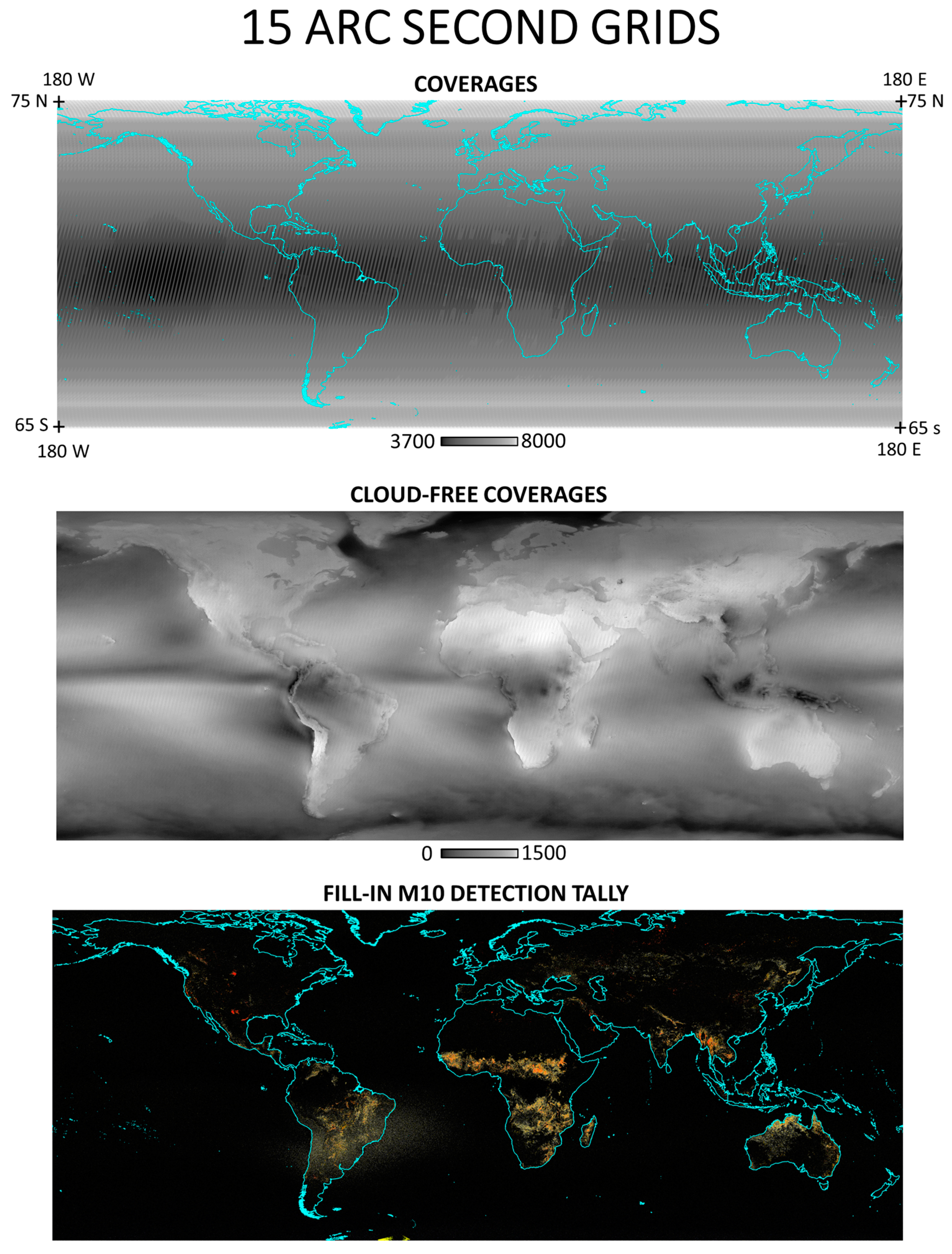
The most challenging aspect of the data analysis was separating detections from industrial IR emitters from the more widespread biomass burning and the atmospheric glow that surrounds large industrial emitters. The approach was to composite cloud-free VNF detections from 2012 through 2022 at 15 arc second resolution and to filter out the biomass burning based on its lower level of persistence as compared with the fixed-location industrial emitters. The filtering process began with the generation of four 15 arc second global grids tallying the total nighttime VIIRS observation (coverages), cloud-free coverages, number of VNF M10 detections, and average VNF temperatures. M10 detections were used instead of M11 because M11 was not collected at night in the early VIIRS record (2012–2017). The other rationale for the selection of M10 for the multiyear compositing of VNF detections was that M10′s band pass coincides with the peak radiant emissions in most gas flares, the predominant type of industrial emitter detected by VIIRS. The cloud-free coverage grid was calculated by subtracting NOAA’s VIIRS cloud detections [22] from the coverage grid. Representations of the coverage and cloud-free coverage grids are shown in Figure 4. The next step was to calculate the percent frequency of VNF detection by dividing the VNF M10 cloud-free detection tally grid by the cloud-free coverage grid. Then the temperature-dependent percent frequency of the detection thresholds was set to separate industrial infrared emitters from ephemeral biomass burning and glow. We refer to the thresholds used to filter out the extraneous detections as “noise floors”.

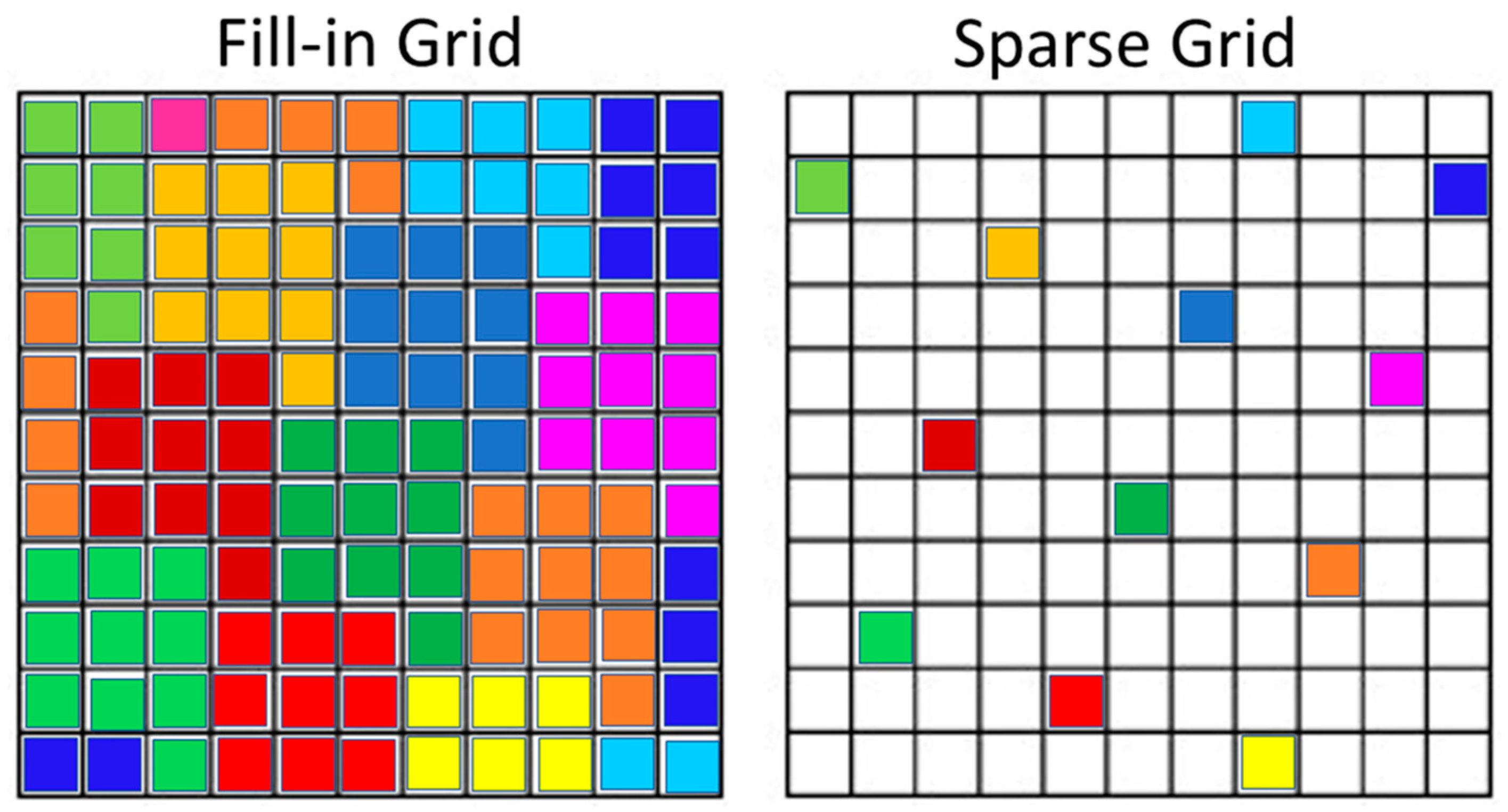
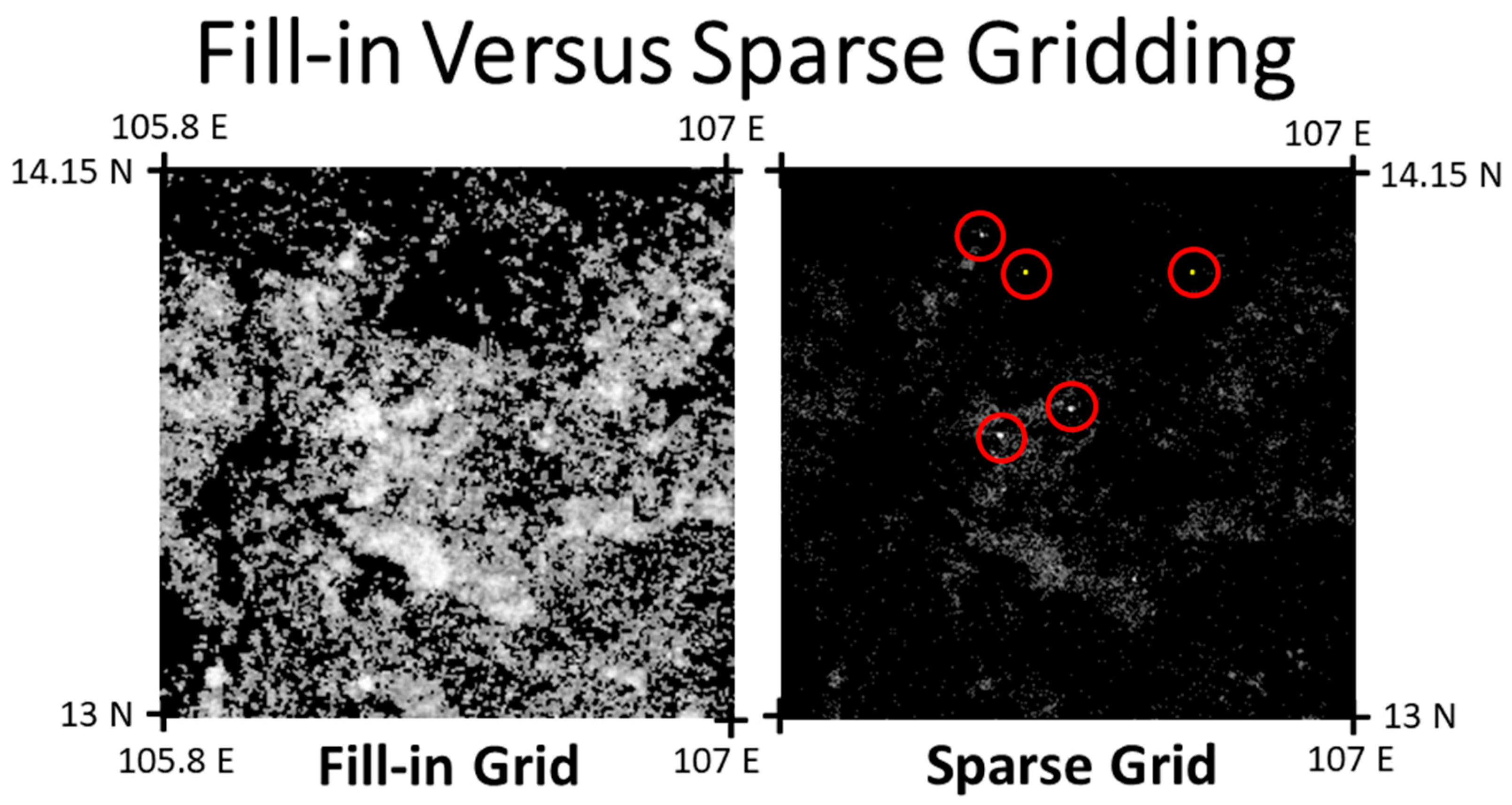
Initially, we attempted to filter out biomass burning using grids assembled with the fill-in gridding method (Figure 5) and all VNF detection pixels. For many years, EOG has used the “fill-in” style of gridding in the assembly of global nighttime lights [7]. This method results in a VNF percent frequency of detection grid that is dominated by biomass burning (bottom panel of Figure 4). With the “fill-in” grid we found that the percent frequency threshold set to eliminate biomass burning also removed many known industrial IR emitters.

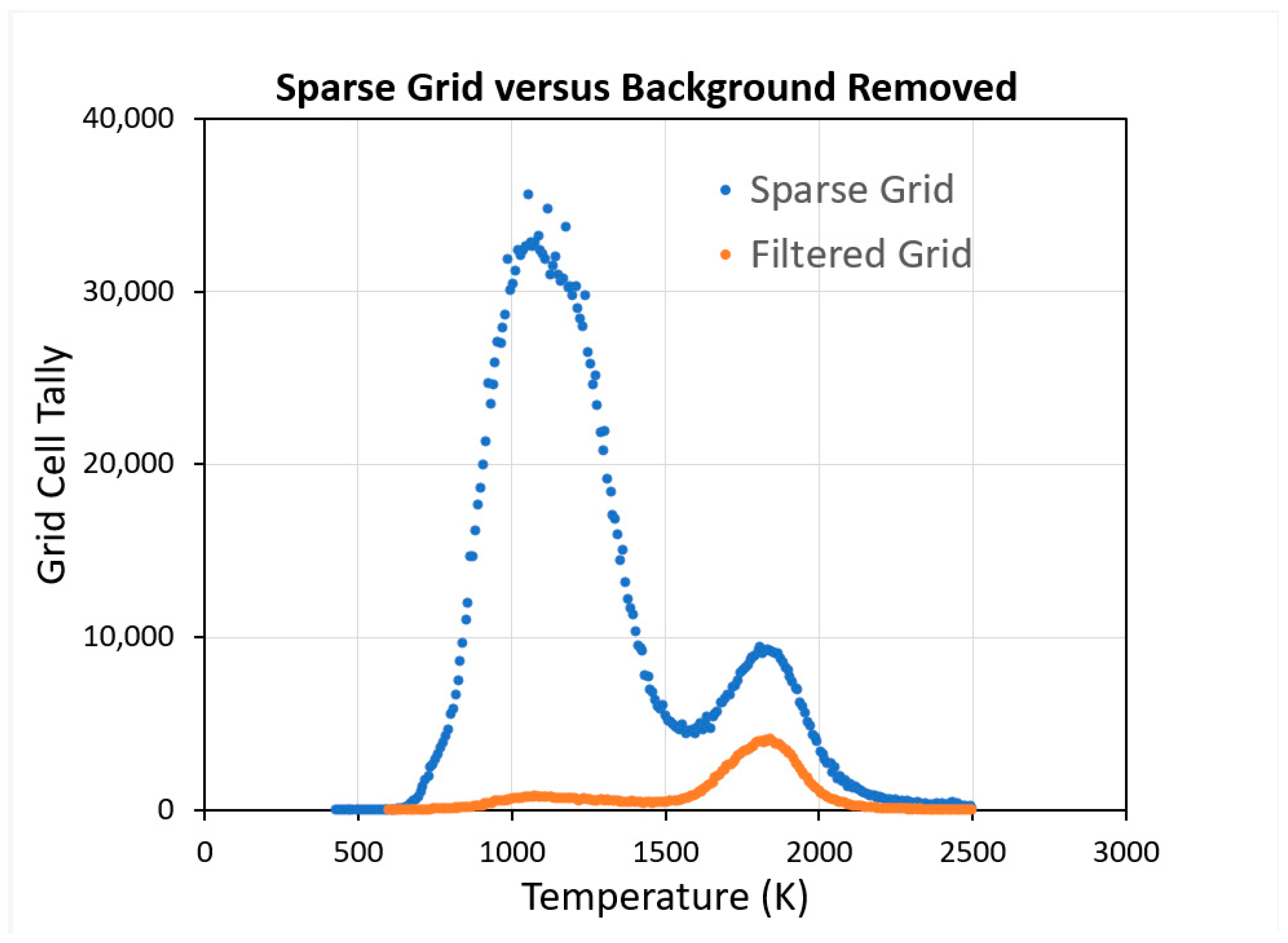
After some experimentation, we decided on two changes in the methodology: (1) only VNF local maxima entered the global multiyear grid and (2) only the 15 arc second grid cells containing VNF pixel center locations were filled in. This style of gridding is referred to as “sparse gridding” (Figure 5). In combination, these two changes in the method vastly reduced the expression of biomass burning and focused the accumulation of industrial IR emitter detections into tightly packed clusters (Figure 6). The sparse grid method had the additional advantage that the VNF records could be gridded globally from the database, without creating intermediate fill-in grids from each sub-orbit prior to global compositing.

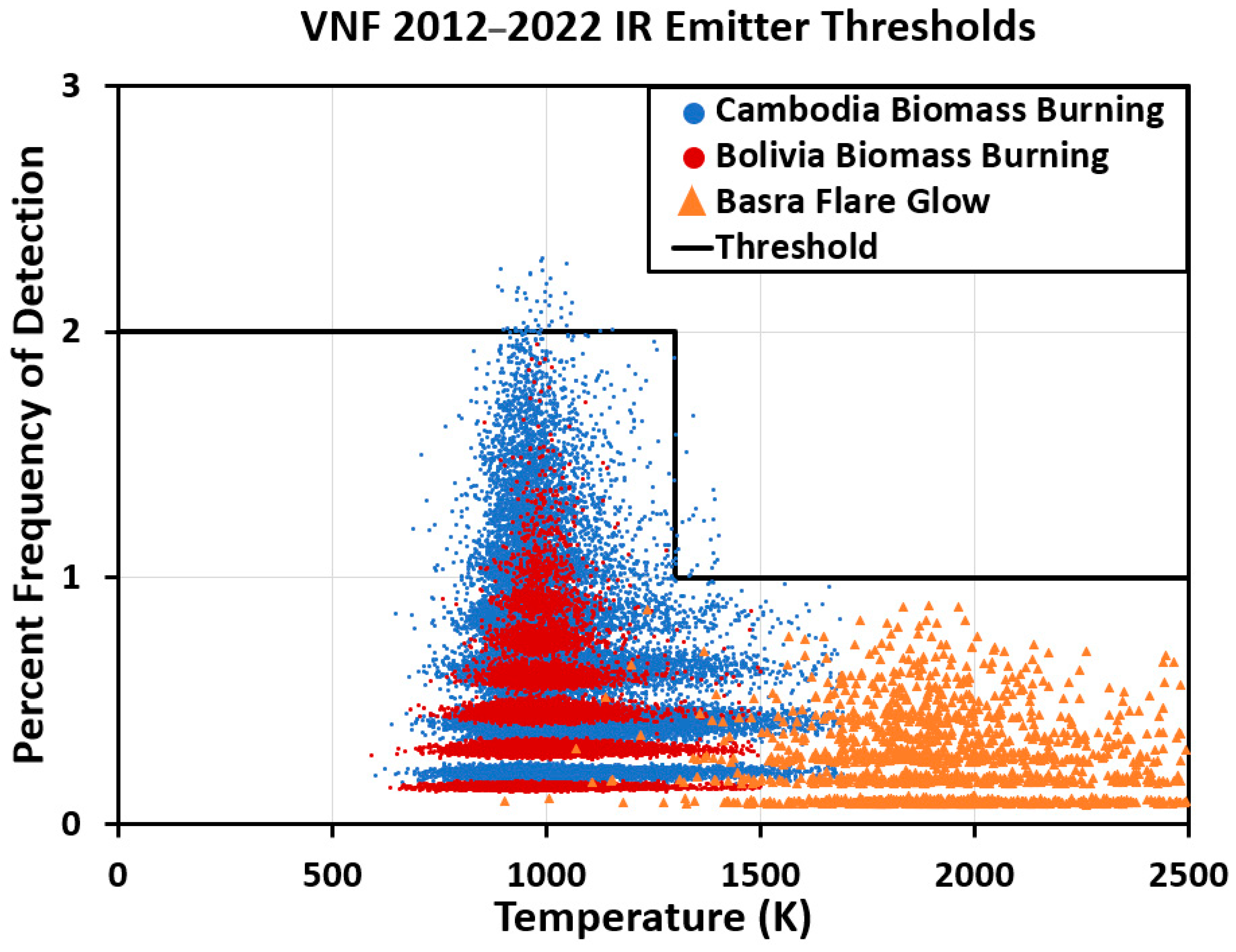
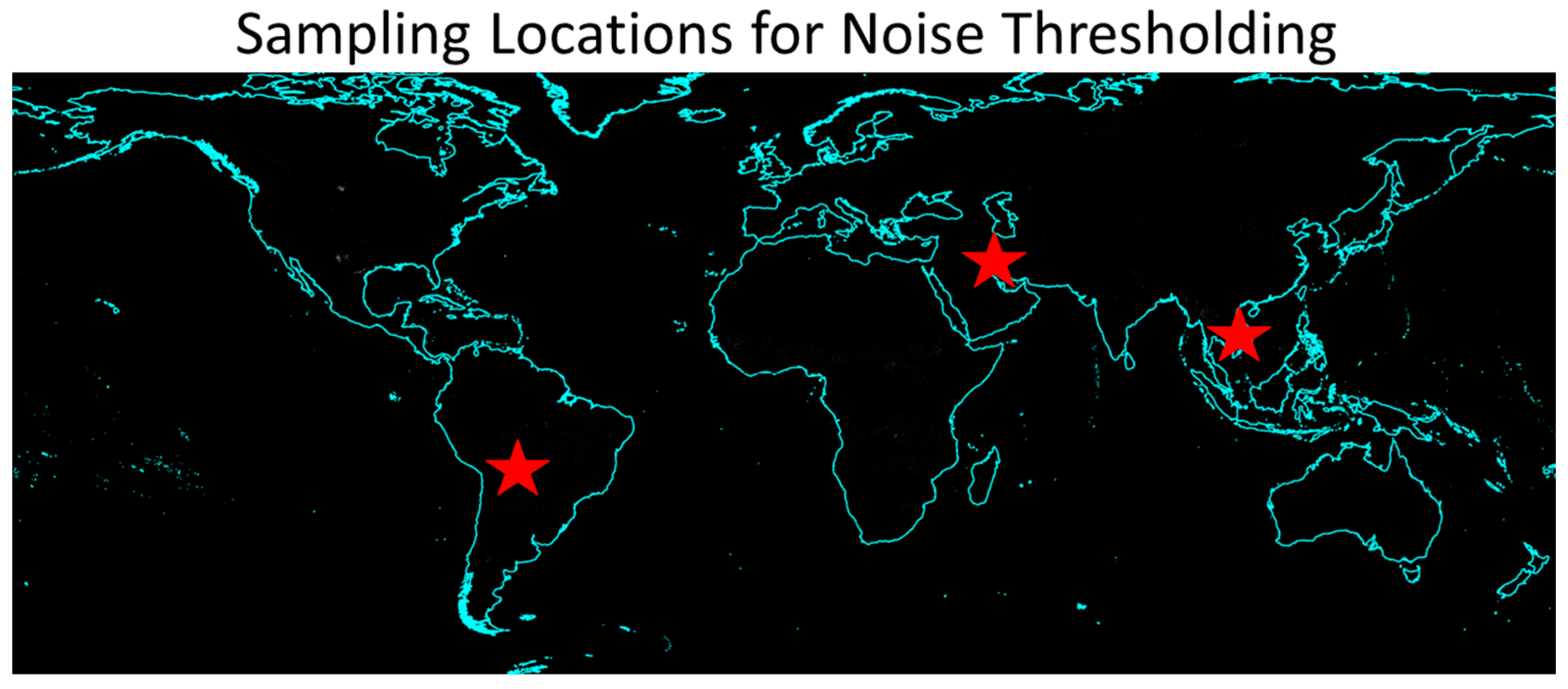
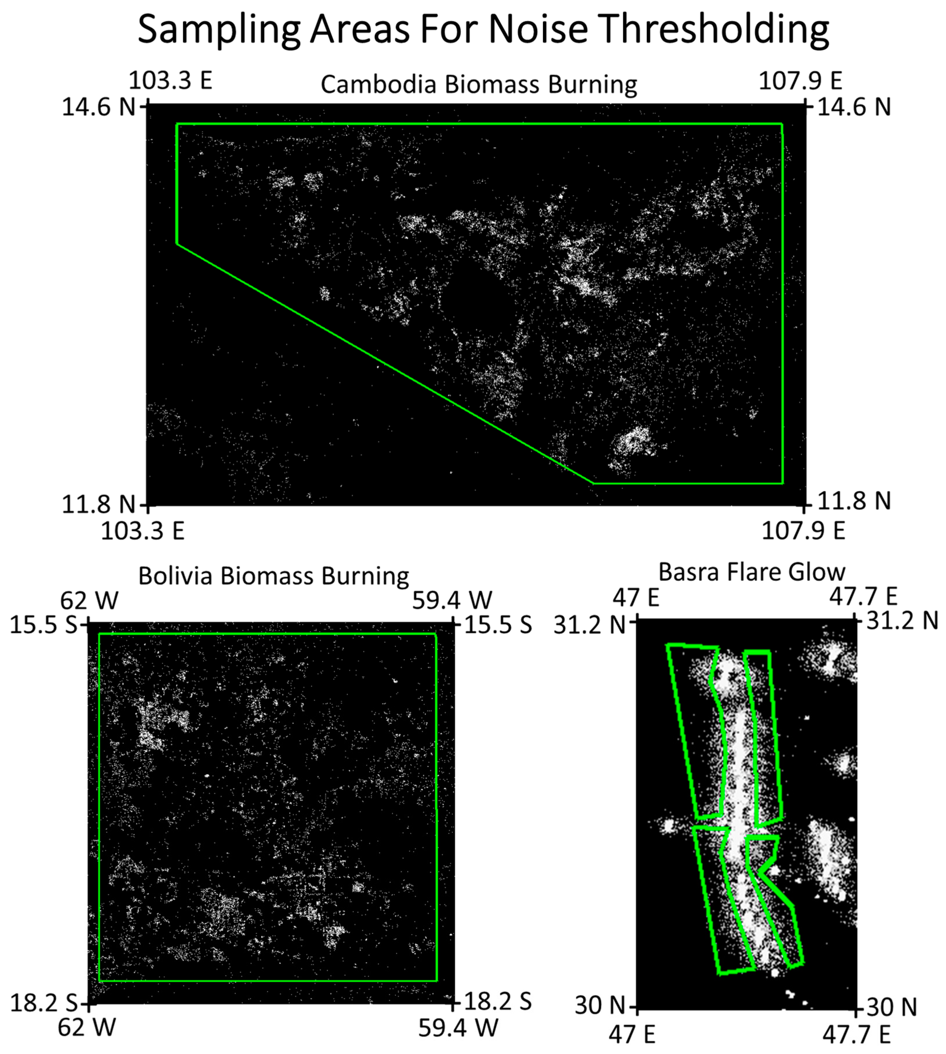
To set the percent frequency of detection noise floor thresholds to separate ephemeral detections from industrial emitters, samples were drawn from three areas having large concentrations of high percent frequency biomass burning and glow surrounding large gas flares. The sampling areas were located in Boliva, Cambodia, and Iraq (Figure 7). Figure 8 shows the cloud-free VNF M10 percent frequency of detection images for the three areas. The noise floor grid cells were plotted on a temperature versus percent frequency of detection scattergram (Figure 9). The selected percent frequency of detection noise floor thresholds was set at 2% below 1300 K and 1% above 1300 K.

3.3. Segmentation

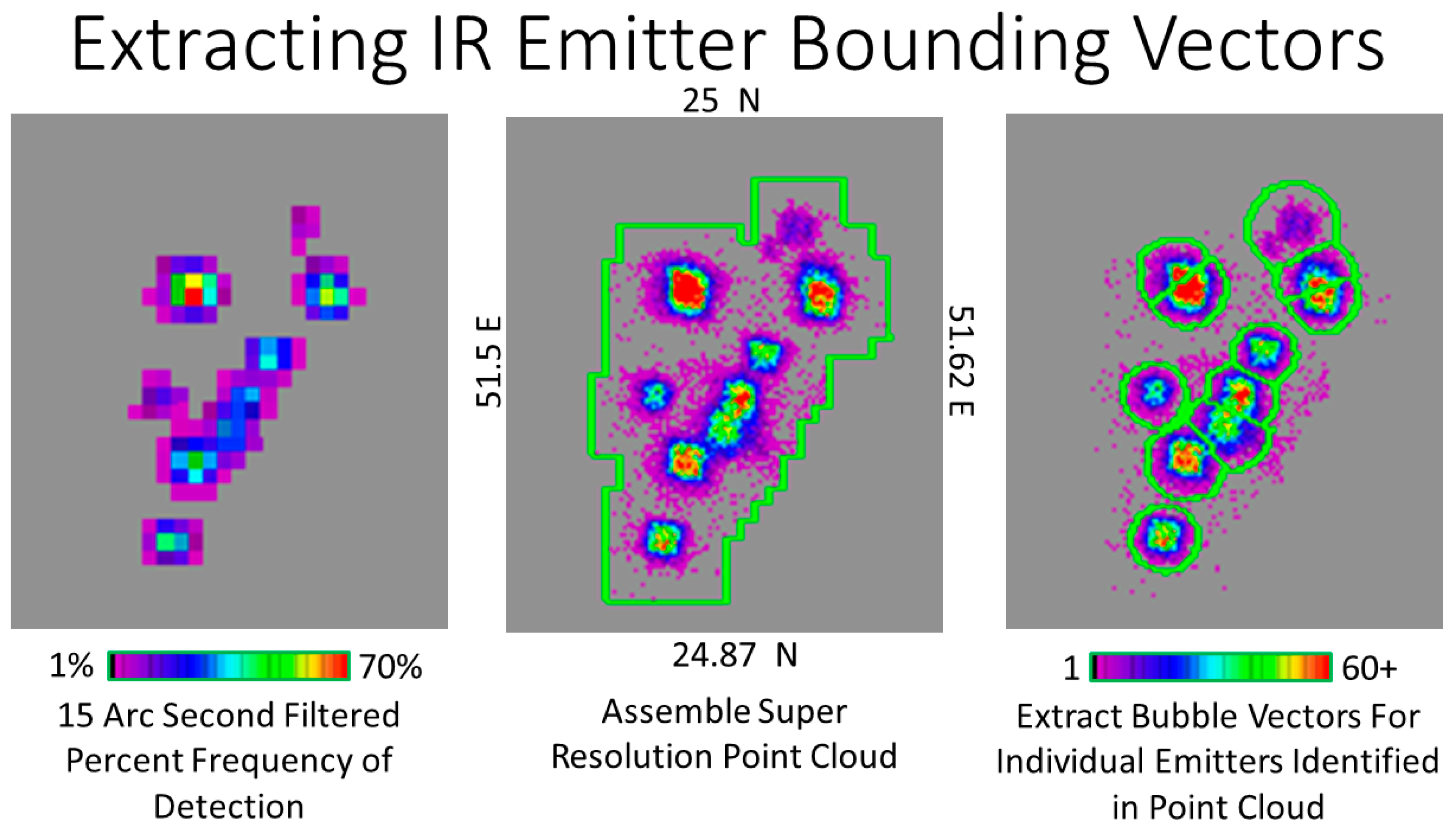
After filtering out the majority of biomass burning and flare glow, a two-grid-cell buffer was applied to each of the IR emitter detection clusters, and vector outlines of the features were extracted (Figure 10). The buffered vector set covering the IR emitters was used to guide the extraction of clear-sky VNF detections from the database, which were then examined for the presence of dense detection clusters that indicated fixed-location IR emitters.

3.4. Super-Resolution Analysis of VNF Pixel Center Locations

The next step in the analysis was performed with the pixel center locations (latitude and longitude) for all clear-sky VNF detections from each of the individual segmentation vectors defined in Section 3.3. Each VNF pixel had a latitude/longitude location calculated for the pixel center, with a terrain correction [23]. The initial filtering to remove biomass burning, described in Section 3.1, was performed with multiyear 15 arc second grids, based on the World Geodetic System (WGS84). However, in pixel center density analysis, we used a flat map Universal Transverse Mercator (UTM) projection. The switch to UTM was performed to reduce the distortion of IR emitter cluster shapes and sizes at high latitudes. The UTM zone for the individual vector polygons was defined by the cluster’s centroid location. The identification of individual industrial emitters and definition of bounding vectors was performed on ungridded pixel center density clouds, a form of super-resolution analysis [24]. Figure 10 shows the transition in spatial resolutions, starting from 15 arc seconds for the initial filtering to pixel center density clouds in UTM projections. To screen out the residual biomass burning clusters that exceeded the 2% detection frequency from the 15 arc second grid, only dense clusters were selected for the definition of persistent IR emitters.

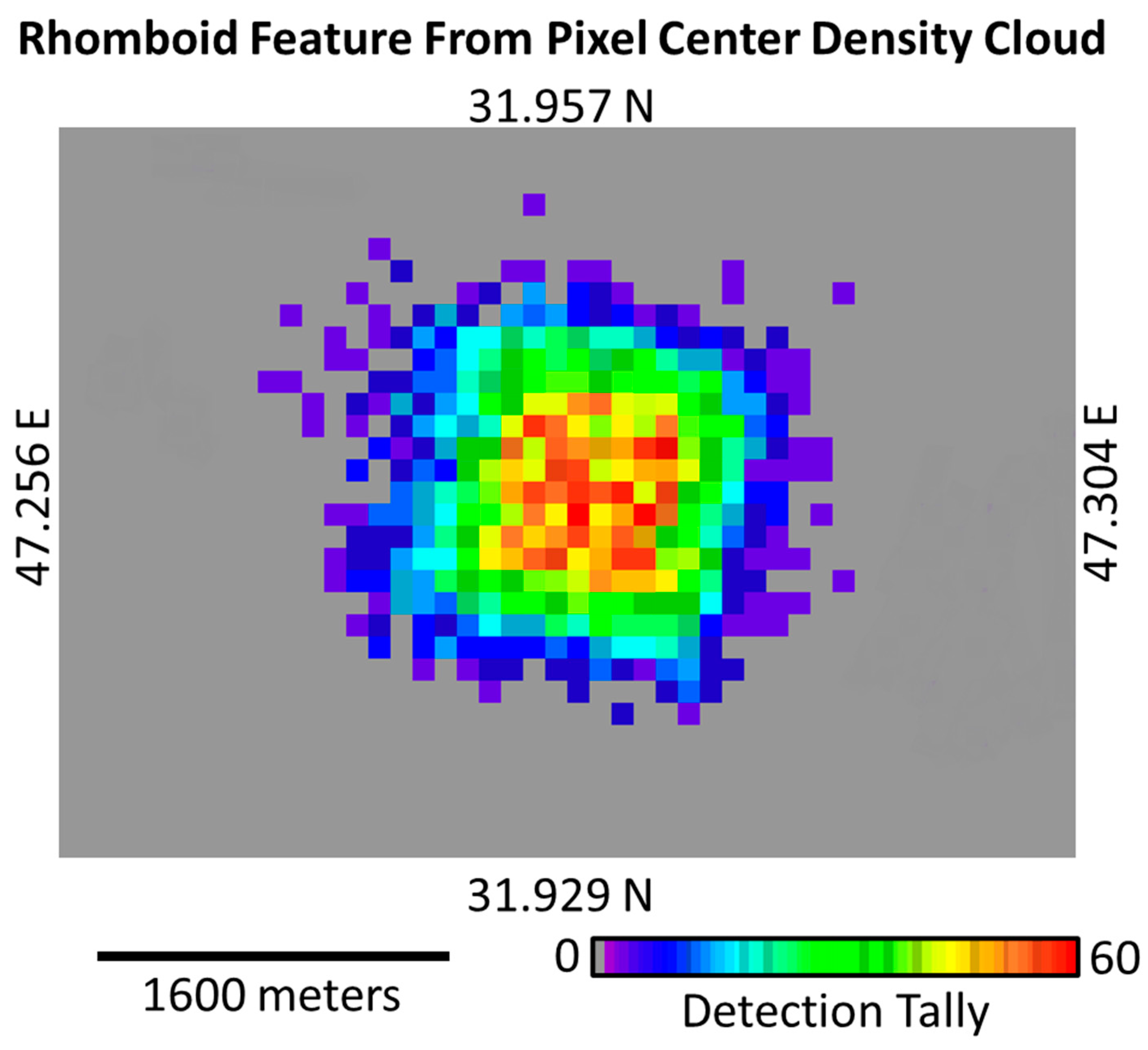
The presence of single frequently detected industrial infrared emitters resulted in a densely packed rhomboid pattern in the pixel center density clouds (Figure 11). The rhomboid’s tilt was the result of the orbit’s precession, set to ensure complete coverage of the Earth two times per day by each VIIRS instrument. This orbital pattern resulted in the VIIRS scanlines being slightly inclined relative to a straight east–west line. The rhomboid shape arose from the fact that the emitter’s position within the pixel footprint was randomized within the time series. In some VNF pixels the emitter was near the center of the pixel footprint, and in other cases the emitter was toward the edge or a corner of the pixel footprint. In addition, the pixel footprint expanded from 742 m on a side at nadir to 1.6 km on a side at the edge of the scan (Table 1). The typical dimensions of the well-developed rhomboids found within the pixel center density clouds were approximately 1600 m high and 1600 m wide, corresponding to the M band resolution at the edge of the scan (Figure 11).

The density and shape of each dense cluster was analyzed with a Variational Bayesian Gaussian Mixture Model (VBGMM) [25] to define the bounding vectors for individual IR emitter features. If the spatial dimensions exceeded 2.6 km² and the shape deviated from the rhomboid found for single emitters (Figure 11), the cluster was split into multiple emitters. The bounding vectors are referred to as “bubble vectors” due to the circular shapes for individual emitters and chord-based splitting of clusters containing multiple emitters.

3.5. Generation of Temporal Profiles

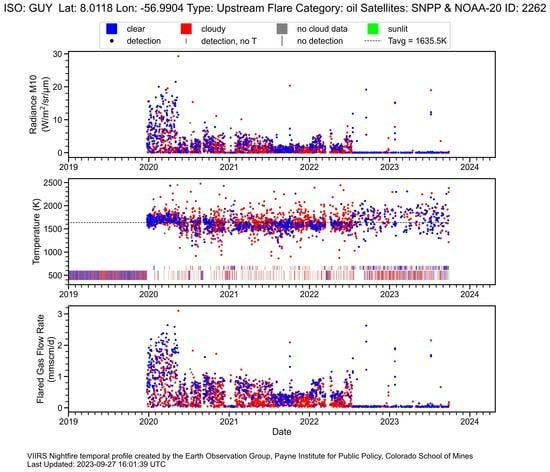
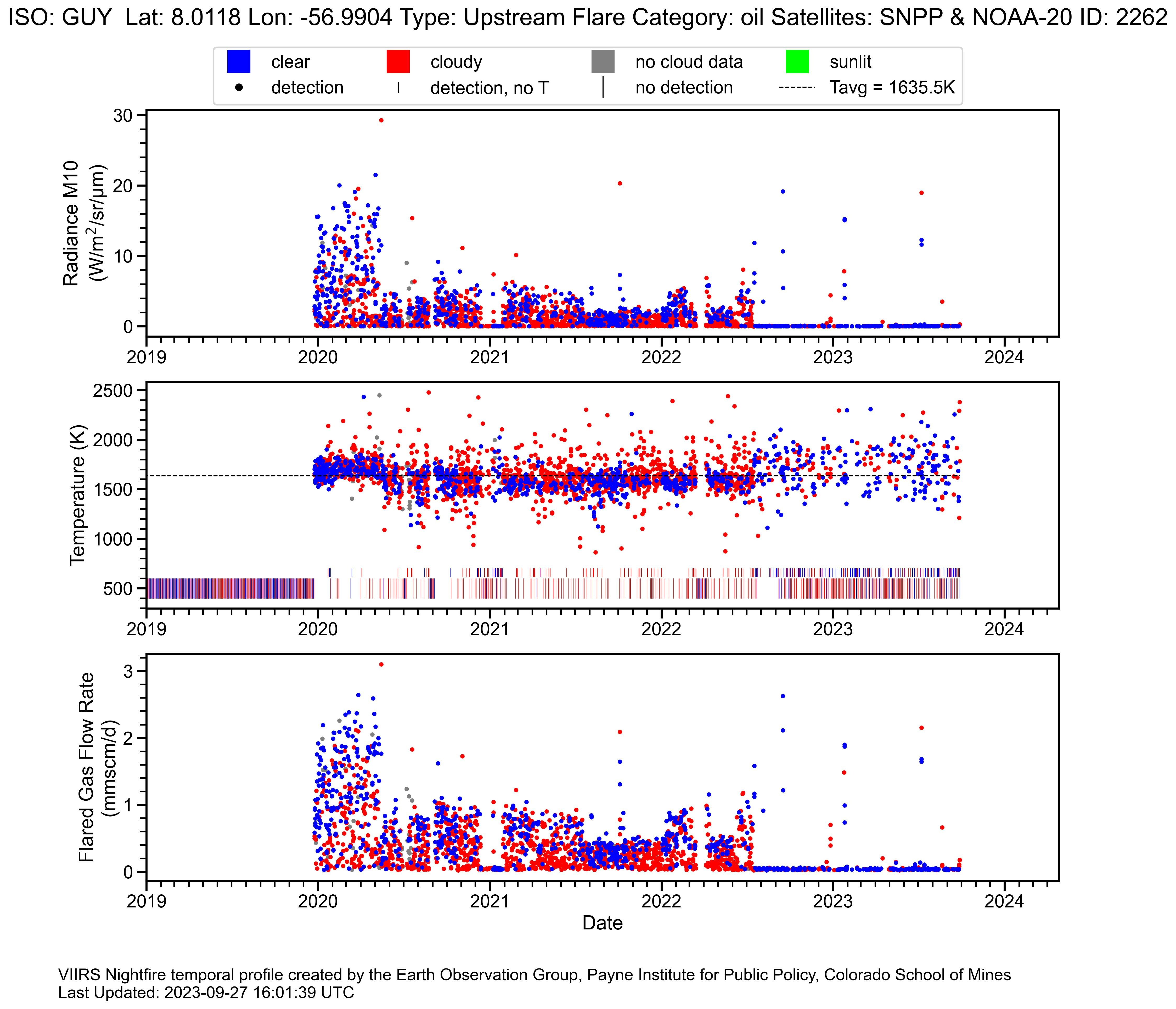
The bubble vectors were used to extract all VNF local maxima from the database, which were arranged chronologically to form temporal profiles. Produced in csv format, the temporal profile is a chronological stack of VNF pixel details, including the name of the M10 source images; latitude; longitude; original line and sample prior to geolocation; band radiances; cloud state; Planck curve analysis results for the temperature, source size, and radiant heat; and for flares, the instantaneous flared gas volume. A graphical summary of the profile was also produced in png format, with a stack of three profiles: M10 radiance, temperature and cloud state, and radiant heat (or flared gas volume for flares). The cloud states were also recorded for VIIRS overpasses where the emitter was not detected.

3.6. Labeling

The emitter types were labeled by geographic cross matching with several emitter catalogs (

Table 2. Catalogs used to label emitter types.

Source	Name	Source
Earth Observation Group	Upstream and downstream gas flares	https://eogdata.mines.edu/products/vnf/global_gas_flare.html (accessed on 1 April 2023)
Global Energy Monitor	Global Steel Tracker	https://globalenergymonitor.org/projects/global-steel-plant-tracker/download-data/ (accessed on 1 April 2023)
Global Energy Monitor	Global Coal Mine Tracker	https://globalenergymonitor.org/projects/global-coal-mine-tracker/download-data/ (accessed on 1 April 2023)
Global Energy Monitor	Global Coal Plant Tracker	https://globalenergymonitor.org/projects/global-coal-plant-tracker/download-data/ (accessed on 1 April 2023)
Pro Global Media Ltd.	Global Cement Directory	https://www.globalcement.com/directory/order-options (accessed on 1 April 2023)
Waste Atlas	Landfills	http://www.atlas.d-waste.com/ (accessed on 1 April 2023)

). The majority of the upstream and downstream flaring sites were labeled based on EOG’s prior single-year flare catalogs [10]. Steel mills, coal mines, and coal plants were labeled based on locations cataloged by Global Energy Monitor. Cement plant locations came from the Pro Global Media’s Global Cement Directory. Landfills were labeled based on locations from the Waste Atlas.

4. Results

4.1. Filtering to Identify Individual Emitter Sites

The most common type of VNF detection is biomass burning. The leverage that we have to identify industrial IR emitters comes from their persistence as measured by the percent frequency of detection within the cloud-free set of detections. To organize the entire mass of multiyear VNF detections for filtering, the detections and coverage tallies were fit into global 15 arc second grids, having 2.9 billion cells (

Table 3. The 2012–2022 filtering to remove biomass burning and glow.

Grid Type	Contour Vector Tallies	Grid Cell Tally	Percent
Empty 15 arc second grid 86,401 by 33,601		2,903,160,001	100%
With cloud-free M10 detections in fill-in grid		93,068,655	3.21%
With cloud-free M10 detections in sparse grid		3,744,797	0.13%
With segmentation vectors applied	14,939	536,240	0.019%
With bubble vectors applied	20,113	233,777	0.008%

). Our first attempt at filtering to separate biomass burning and industrial emitters was conducted with VNF detections fit into the global grid using the fill-in method used previously in generating global nighttime lights. We found that the fill-in process magnified the spatial extent and percent frequency of biomass burning. Thus, we switched to only gridding VNF local maxima and using a sparse grid, where only the grid cells containing VNF pixel centers were filled. This vastly reduced the number of grid cells to be filtered from 93 million down to 3.7 million. The biomass burning and a portion of the glow surrounding the emitters was filtered out using a 2% detection frequency threshold for grid cells averaging less than 1300 K and a 1% threshold for grid cells averaging more than 1300 K. The remaining grid cells were segmented into 14,939 clusters for further analysis via pixel center density maps. Individual industrial IR emitter sites were identified as dense assemblages of VNF detections located within the pixel center density maps.

In total, 20,113 IR emitter sites were identified, spread across 143 countries. The country having the largest number of emitters was the USA, with more than 6000 (

Table 4. The 2012–2022 VIIRS IR emitter tallies by country.

Country	IR Emitter Tally
United States	6094
China	2848
Russian Federation	2280
Canada	787
India	593
Iran	540
Indonesia	431
Brazil	347
Nigeria	290
Egypt	281
Iraq	280
Argentina	278
Algeria	271
Mexico	266
Saudi Arabia	266
Kazakhstan	198
Venezuela	192
Australia	186
Colombia	185
Ukraine	149

). China had about half as many emitter sites as the USA, and Russia had about a third as many emitter sites as the USA. The most abundant emitter type was the upstream gas flares, comprising 67% of the total (

Table 5. IR emitter tallies by type.

IR Emitter Type	Tally
Upstream gas flares	13,449
Downstream gas flares	1535
Metallurgy	1732
Industrial TBD	1344
Coal mines and power plants	558
Unknown	528
Wood processing	297
Landfills	279
Volcanoes	92
Cement factories	83
Unique	4
Greenhouses	4
TOTAL	19,905

). Upstream refers to flares in oil and gas production areas, while downstream refers to flares at refineries or other processing sites.

4.2. Temperature Histograms

Early on [9,26], it was recognized that the global VNF temperatures followed a bimodal distribution, with a broad peak near 1100 K dominated by biomass burning and a second shorter peak near 1800 K arising from natural gas flaring. This was evident in the temperature histogram generated from the fill-in grid version of the average temperature (Figure 12). By suppressing the expression of biomass burning, the relative proportions of the two peaks shifted away from the lower temperature peak in the sparse grid version of the average temperatures (Figure 12).

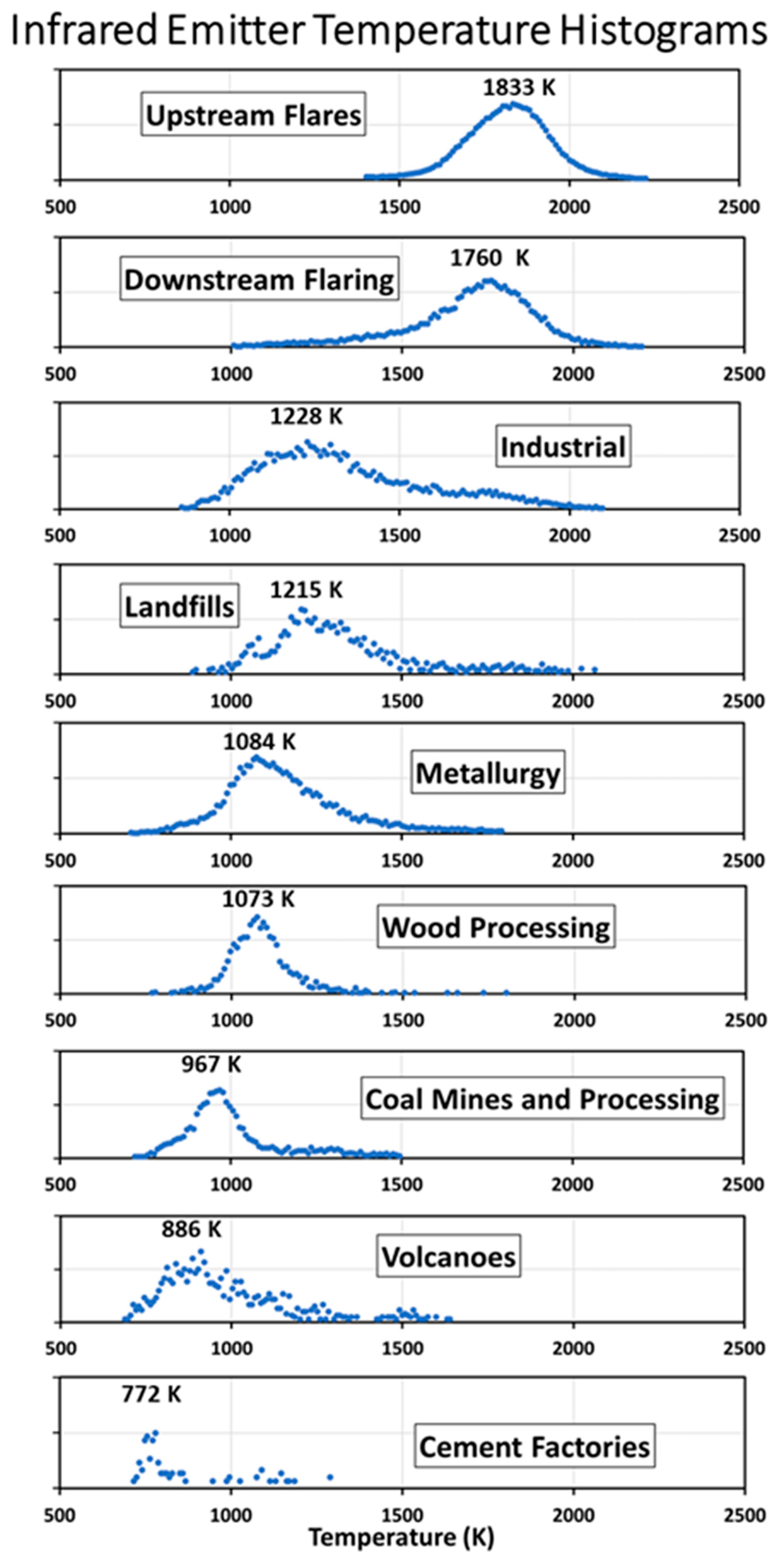
Global temperature histograms were produced for nine major emitter types (Figure 13). The temperature mode was provided for each of the histograms. The emitters could be broadly divided into a hot set arising from natural gas flaring and a cooler set having a similar temperature range to biomass burning. The upstream and downstream flaring was primarily in the range of 1500 to 2200 K. The temperature mode for the industrial emitter type was 1228 K. However, there were industrial sites that also had flaring, indicated by detections in the 1500 to 2200 K range. Landfills had a temperature mode of 1215 K and also had evidence of flaring, exhibited as a long tail on the hot side of the distribution, from 1500 to 2000 K. The metallurgy group was primarily steel mills, with a temperature mode of 1084 K and a slightly higher temperature tail as compared with landfills. The wood processing emitter type’s mode was 1074 K, nearly the same as metallurgy but with less of a tail on the high-temperature side. The coolest emitter type, under 1000 K, included coal mines, volcanoes, and cement factories.

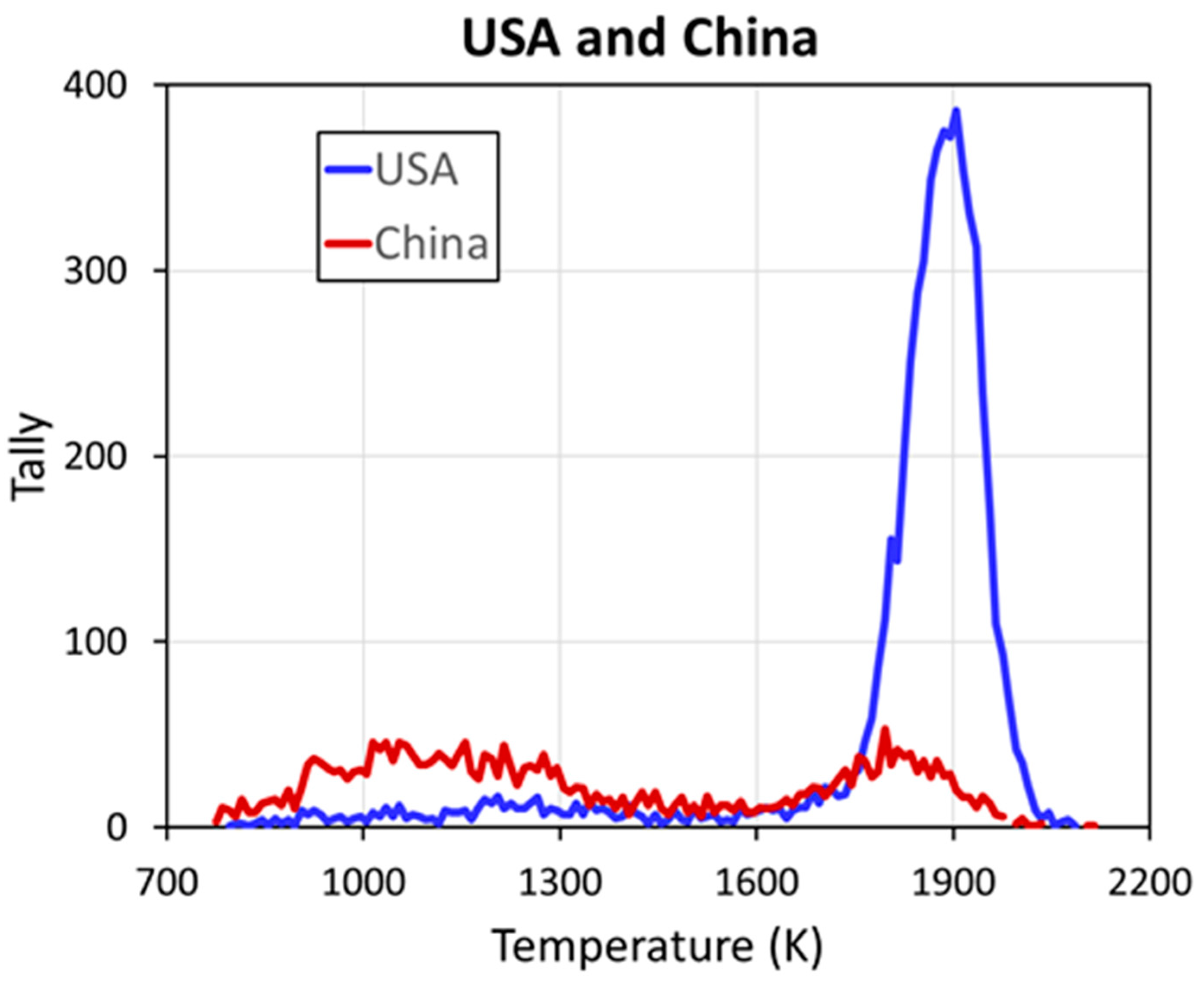
IR emitter temperature histograms were also generated for each country. Figure 14 shows the temperature histograms for the USA and China; the two countries accounted for more than 40% of the infrared emitter sites. The USA temperature histogram was heavily skewed toward hot natural gas flaring sources, with far fewer lower-temperature industrial emitters. China was the opposite, with a preponderance of industrial-style emitters in the range of 800 to 1300 K.

4.3. Nightly Temporal Profiles

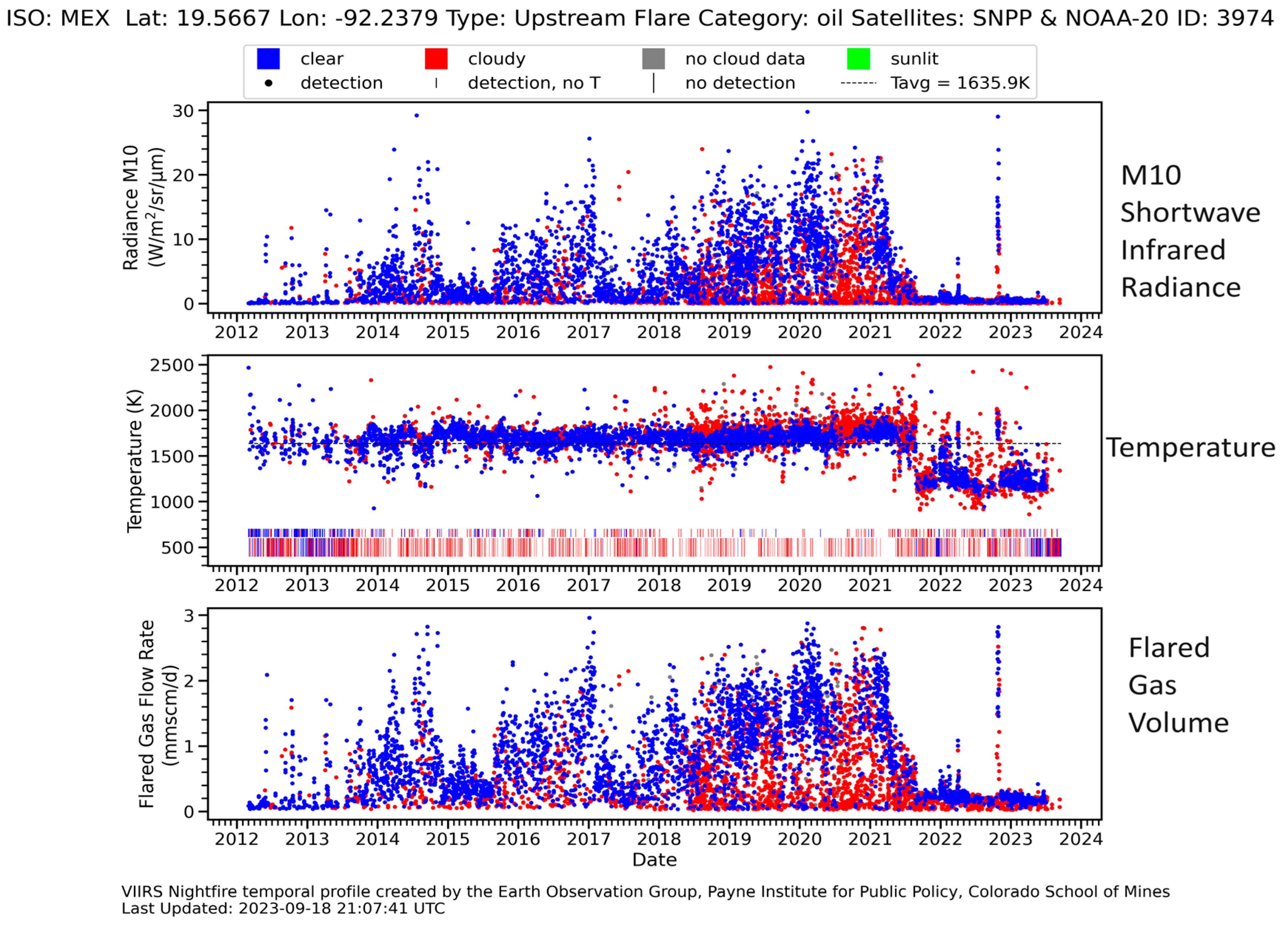
Nightly temporal profiles were assembled for each of the IR emitter sites. These revealed the activity patterns and temperature ranges of the sites. Figure 15 shows an example of a temporal profile from an offshore gas flare in Mexico. The nightly emitter dashboard includes three stacked charts: (1) the SWIR M10 radiance, (2) the temperature in Kelvin, and (3) the radiant heat in megawatts. For gas flares the RH chart was replaced by flared gas volumes in terms of methane equivalents. The clear-sky observations are marked in blue, and the cloudy observations are red. Note that the activity levels were relatively low in 2012–2013 and had several bursts of higher flaring activity in 2014, 2016, and 2019–2021. The M10 radiance dropped to a much lower level toward the end of 2021 with a temperature drop at the same time. The temperature drop indicated the site stopped flaring, although a lower-temperature emitter continued to be detected. These changes may have been associated with the installation of new hardware to use the flared gas onsite.

4.4. National-Level Monthly Temporal Profiles

Monthly tallies of active infrared emitters and cumulative heat output (radiant heat) were produced for the countries of the world. These were generated for the individual emitter types, as listed in Table 5, and a version was also generated combining all emitter types. Here we present several “all-emitter” monthly profiles (Figure 16, Figure 17, Figure 18, Figure 19, Figure 20 and Figure 21) to illustrate the changes in activity levels, obscuration, effects of military conflict, and COVID lockdown effects.

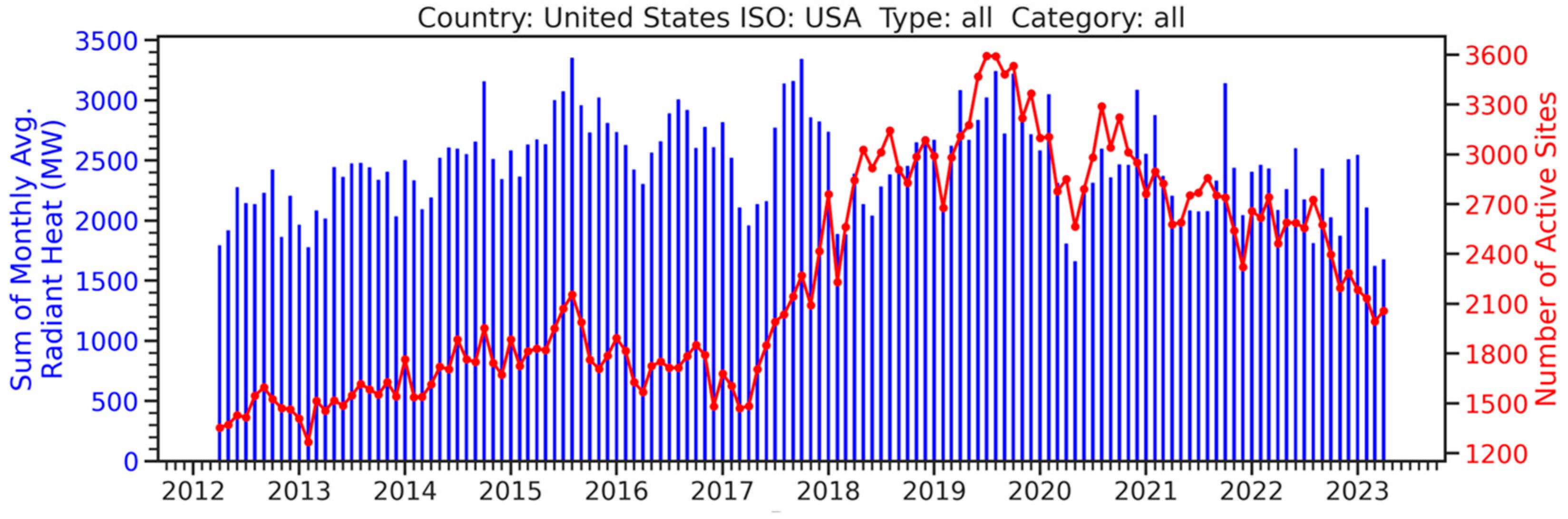
Figure 16 shows the monthly temporal profiles for all identified industrial IR emitters in the USA, where upstream natural gas flaring dominated the emitter types. There was a steady increase in active emitter numbers from May 2017 to August 2019, corresponding to an expansion in the number of upstream gas flares in oil-shale production areas such as Texas and North Dakota. Activity levels gradually dropped in 2020 through 2022. There was also a dip in the number of active sites and radiant heat from March through July 2020, corresponding to the COVID lockdown in the USA.

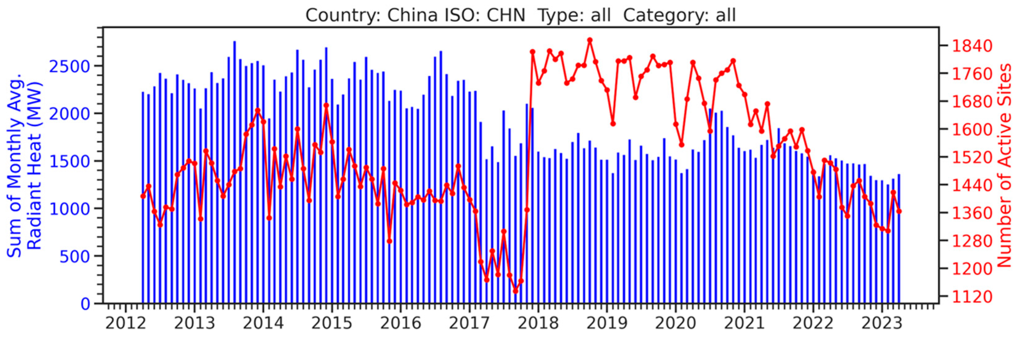
Figure 17 shows the monthly temporal profile for industrial IR emitter activity for China, the country with the second largest number of industrial IR emitters. There was a dip in IR emitter activity from March through October 2017 followed by a steep increase in the number of active emitters beginning in December 2017. We attributed this increase in active IR emitters to the addition of nighttime M11 in both the SNPP and NOAA-20 VIIRS collections. M11 was in the shortwave infrared (SWIR) and had the lowest detection limits for IR emitters above 1000 K of any of the VIIRS bands [26]. Thus, adding M11 resulted in larger numbers of dim emitters yielding temperature fits from the VNF Planck curve fitting.

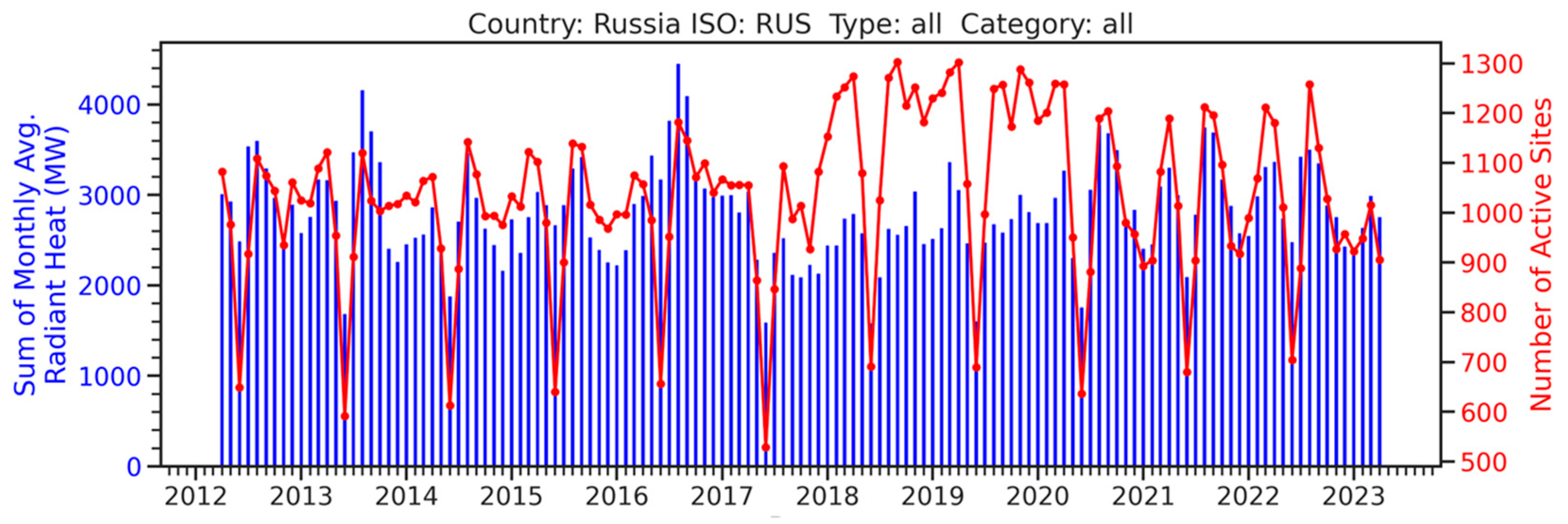
Figure 18 shows the monthly temporal profile of industrial IR emitter activity for the Russian Federation, the country with the third largest number of IR emitters. Here we found annual cycling, with sharp dips in the active site tally and radiant heat each year during May, June, and July. This was due to solar contamination centered on the Northern Hemisphere’s summer solstice. With an after-midnight overpass, VIIRS was less prone to this problem than the DMSP Operational Linescan System, which had an overpass time between 19:00 and 22:00 [7]. As with China, there was evidence of an increase in the number of active sites starting in December of 2017, associated with the addition of the second SWIR channel, M11. The mid-winter dips in activity levels were more pronounced in 2020 and 2021, perhaps an expression of COVID impacts on gas flaring activity. Alternatively, this may have been an artifact of the change in the cloud detection settings used by EOG.

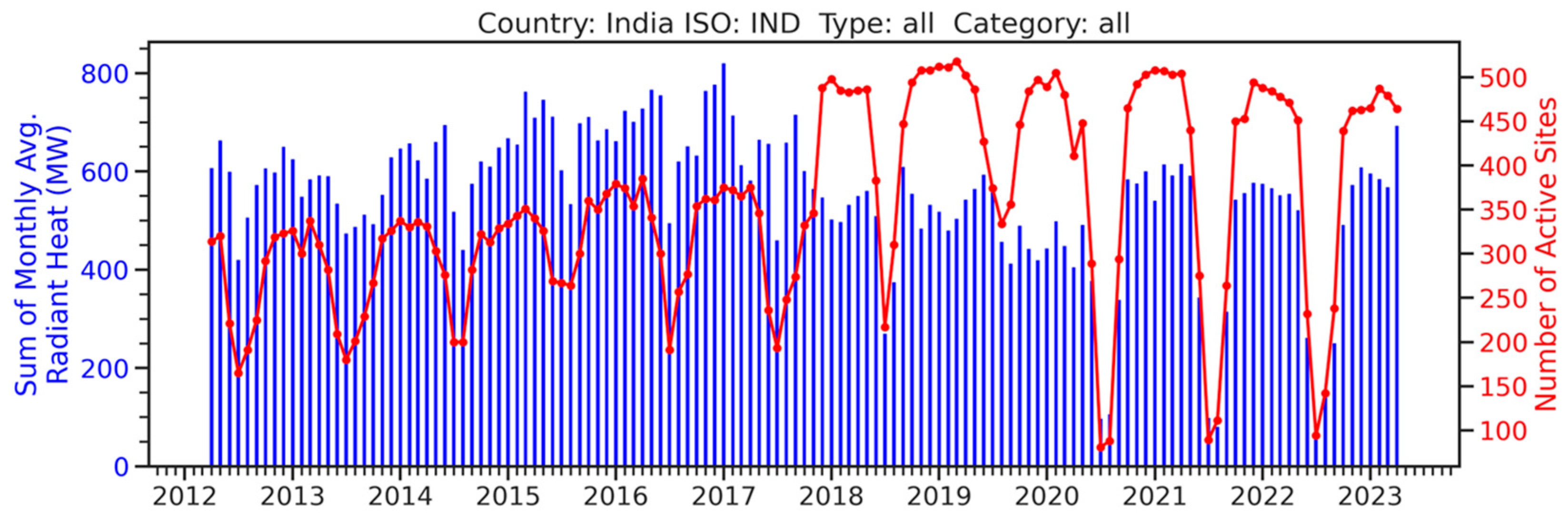
Figure 19 shows the monthly IR emitter activity levels for India. Here heavy cloud cover during the Indian monsoon resulted in reduced numbers of active sites in June through September. As with China, there was a boost in the number of active IR emitter sites in December of 2017, corresponding with the start of nighttime M11 collections. The monsoon dips during 2020 and 2021 were unusually deep, perhaps associated with a change in NOAA’s cloud detection algorithm.

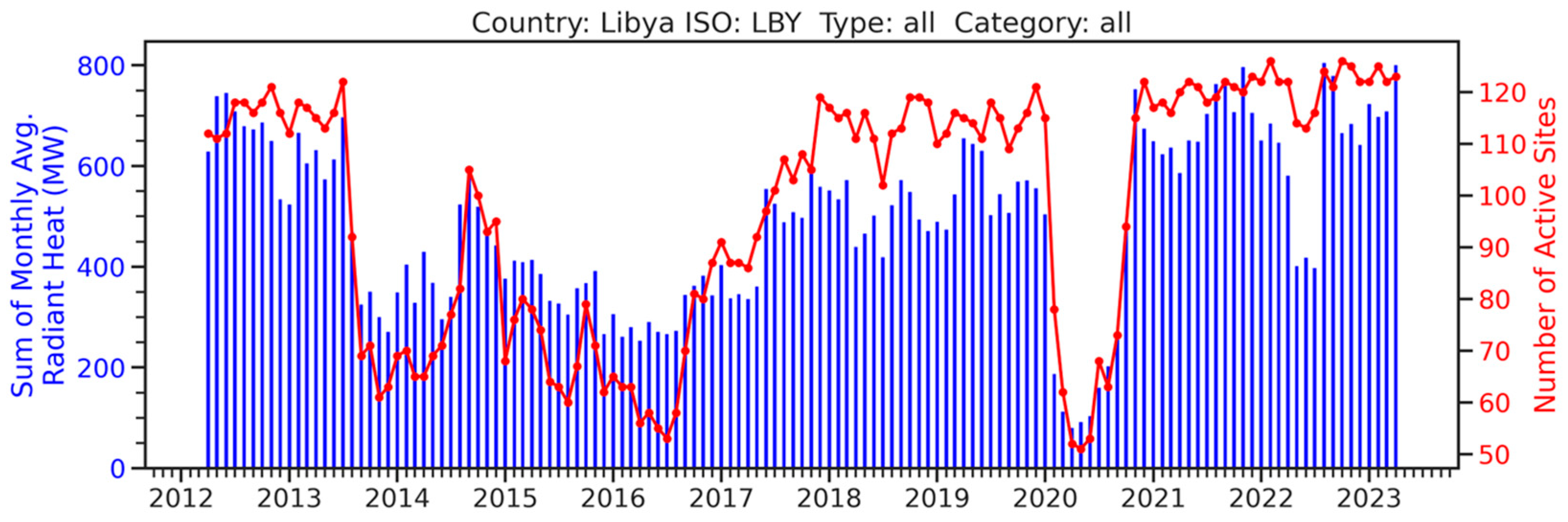
Libya’s monthly temporal profile (Figure 20) was primarily dominated by upstream and downstream natural gas flaring. The Libya temporal profile was fraught with declines in the numbers of active emitters and radiant heat induced by civil war, instability, and COVID. The first major decline occurred in June 2013, followed by a partial recovery in the second half of 2014. A second period of decline occurred in 2015–2016 followed by recovery in mid-2017 to the end of 2019. Libya exhibited one of the best expressions of the decline in economic activity associated with COVID lockdowns, with a deep “U”-shaped decline in both the number of active emitters and radiant heat from February through August of 2020. There was an additional period of decline during May–June–July of 2022.

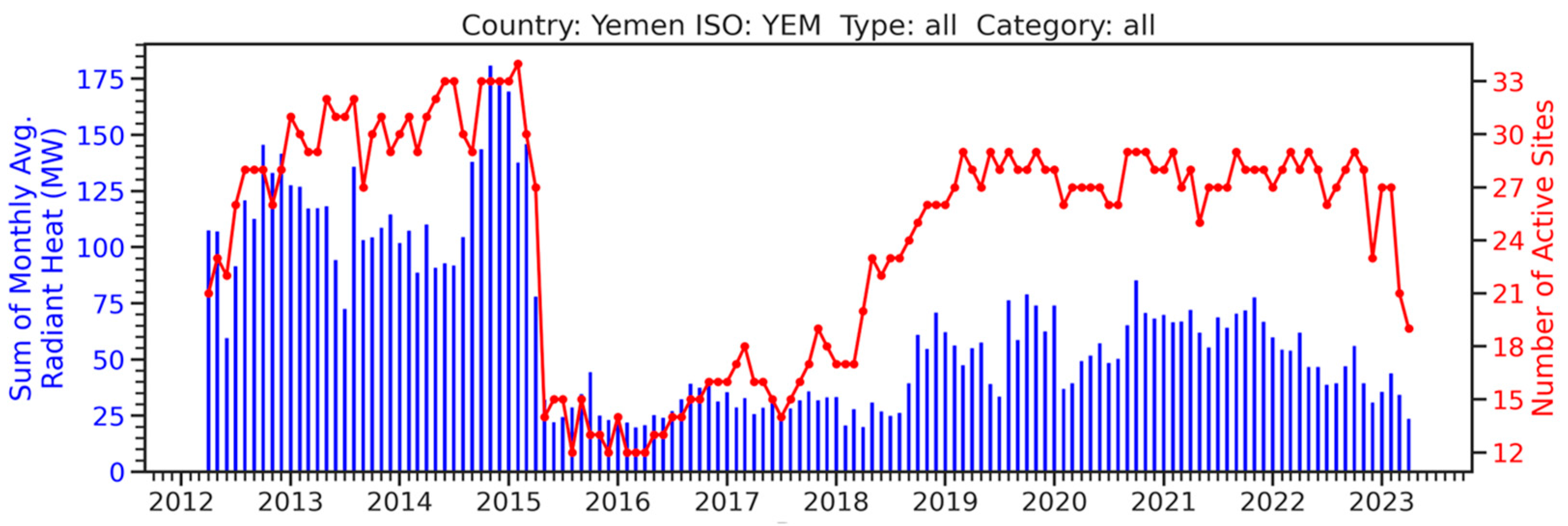
Yemen’s monthly IR emitter profile (Figure 21) showed a sharp decline in both numbers of emitters and heat output in March of 2015, when the country was subjected to intense aerial bombardment. The recovery has been slow due to the prolonged nature of the conflict between Yemen and Saudi Arabia.

5. Discussion

The vast majority of VNF detections were from ephemeral biomass burning, with shifting locations over time. To minimize the expression of biomass burning, we used sparse gridding to build global 15 arc second grids tallying the number of M10 detections and the average temperature. From there, a two-stage process filtered out biomass burning, leaving fixed-location infrared emitters. The first stage was performed with global 15 arc second grids of the percent frequency and average temperature of all cloud-free VNF detections spanning 2012–2022. A 2% frequency of detection threshold was applied for grid cells under 1300 K, and a 1% threshold was applied to grid cells 1300 K and hotter. After thresholding, the outlines of the remaining detection clusters were defined, and a narrow buffer was applied to ensure all VNF detections associated with industrial infrared emitters were considered in defining the sites. Super-resolution VNF pixel center density clouds were generated for each of the 15 arc second segmentation vectors. The pixel center density clouds were analyzed to distinguish fixed-location IR emitters from sparse and random biomass burning. Centroids were recorded as the locations for emitters, and bounding bubble vectors were defined for each of the identified emitters.

There were three changes in the VNF temporal record that users should be aware of. First, only a single SWIR band—M10—was operated at night from 2012 through November 2017. M11 collections commenced in December of 2017 for both the SNPP and NOAA-20 VIIRS instruments. VNF calculations of temperatures, source areas, and radiant heat could only be performed for pixels having detection in at least two spectral bands. Every night, there was a population of single-band detections, unsuitable for Planck curve fitting, for which the temperature could not be calculated. EOG refers to these as “white ghosts”. From 2012 to November 2017 the white ghost detections were in M10. Because the M11 detection limit was lower than that of M10 [24], all pixels having M10 detection will also have M11 detection, making the Planck curve fitting possible. The lower detection limit of M11 brought in a new cadre of industrial emitters too dim to be detected in M10 or M12–M13. This resulted in a step up in the number of active emitters in the monthly temporal profiles of China and India (Figure 17 and Figure 19).

The addition of M11 also affected the variance in the VNF temperature calculations beginning in December 2017. The added temperature variance traced back to the “SWIR-only” pixels, where there was close spectral spacing of M10 (1.63 µm) and M11 (2.2 µm). The temperature calculations stabilized when additional spectral bands were added from spectral bands at either shorter (M7 and M8) or longer wavelengths (M12–M13). A similar temperature instability existed from VNF pixels having only M12 and M13 detection, again attributable to the close spacing of the M12 and M13 band passes.

The second event leaving an imprint on the temporal profiles was the addition of VNF detections from the NOAA-20 VIIRS, which began producing data in early December 2017. This doubled the density of VNF detections in the temporal profiles.

A third factor impacting the temporal profiles was a change in the cloud detection product used in labeling clear and cloudy VNF detections in the latter part of the current temporal record. From 2012 through 2019, EOG used the VIIRS Cloud Mask (VCM)—a bit mask with values ranging from 0 to 3—with 0 indicating confidently clear, 1 indicating probably clear, 2 indicating probably cloudy, and 3 indicating confidently cloudy. EOG lumped 1 and 2 to label clear VNF detections and 2 and 3 to label cloudy. In 2019, NOAA introduced a new algorithm for cloud detection and discontinued the VCM product line, replacing it with a cloud-probability product with values ranging from zero to 100%. EOG set a threshold of 25% cloud probability to distinguish clear from cloudy. This resulted in the over-detection of clouds, primarily in tropical areas having chronically high levels of cloud cover. As a result, EOG has embarked on the development of a cloud detection algorithm optimized for labeling clear versus cloudy for infrared emitters. Later, EOG plans to reprocess the full VIIRS archive with the new cloud algorithm and apply an atmospheric correction to all VNF detections.

Finally, temporal profiles from high-latitude sites had detection gaps due to solar contamination when the satellite zenith angle dipped below 95 degrees. In these cases, the sun was over the horizon, but there was enough solar glow to render VNF’s M7 to M11 detection algorithm useless. The presence of trace quantities of sunlight also disrupted the background diagonal used in the M12–M13 detector [18]. The classic example of solar obscuration is the temporal profile of Russia, shown in Figure 18.

6. Conclusions

We report on the first daily global satellite monitoring program for natural gas flaring and thermal activity levels at industrial sites based on infrared radiant emissions. Nearly 20,000 industrial sites were cataloged, and nightly temporal profiles were produced for each. While we are not the first group to develop catalogs of industrial infrared emitters from space, we are the only group to have operationalized the update of the temporal and radiant heat profiles and to provide access to these via a web map service.

This development was based on multispectral nighttime data collected in wavelengths spanning from 0.8 to 12 µm by the NASA/NOAA Visible Infrared Imaging Radiometer Suite. The VIIRS nightfire (VNF) algorithm relies heavily on four daytime infrared channels that continue to collect at night. With sunlight eliminated, the channels serve as super-detectors for industrial activity where waste heat is exposed to the sky. For sites with detections in two or more channels, VNF calculates the temperature, source size, and radiant heat using physical laws.

The major challenge in this development was the filtering to exclude biomass burning, which was the most common type of VNF detection. To identify the persistent infrared emitters, we used two separate filtering stages. The filtering was akin to finding “needles in a haystack”. The “needles”, or industrial infrared emitters, were identified based on their sharp focus into clusters of closely spaced detections and persistence, as compared with biomass burning. The “haystack” was the vast numbers of ephemeral and sprawling biomass burning and cooler background areas lacking VNF detection.

The first of the filtering stages focused on dropping out the biomass burning. This filtering was performed on a pair of cumulative 15 arc grids tallying the number of shortwave infrared (M10) detections and average temperature. The grids were constructed using local maxima detections extracted from the VNF database, with the number of detections and average temperature recorded. To establish filtering thresholds, pixel sample sets were extracted from areas having more frequent biomass burning and glow surrounding major flares. For sites having temperatures below 1300 K, a persistence threshold of 2% effectively filtered out biomass burning. Sites above 1300 K were primarily gas flares, which in some cases were surrounded by a dim glow from atmospheric scatter. From 1300 K and above, the persistence threshold could be dropped to 1%.

These thresholds did not remove all the biomass burning or flare glow detections but thinned them out to a level at which a second process could be used to identify tightly packed clusters of VNF detections indicating the presence of fixed-location IR emitters. The grid cells that passed this initial filtering were then segmented into individual clusters for super-resolution analysis based on the precise latitude/longitude VNF pixel centers covered by the 15 arc second clusters. We built pixel center density clouds in a UTM projection and analyzed these to identify individual IR emitter features. In some cases, a 15 arc second IR emitter cluster yielded a single tightly packed feature from the pixel center density cloud. In other cases, 15 arc second detection clusters yielded multiple IR emitters. A circular bounding vector was established for each of the identified IR emitters. In cases where these circular vectors overlapped, the circular vectors were split using chord lines connecting the intersection points.

The multiyear VNF IR emitter catalog includes 20,131 sites, and 30% of these are found in the USA. Other countries having large numbers of IR emitters include Russia, China, Canada, and India. Nine major types of industrial emitters have been found: upstream and downstream flaring, industrial, metallurgy, landfills, coal mines and processing, wood processing, and cement factories. In addition, there is an “unknown” group of emitters whose types have yet to be identified. Over time we plan to improve the emitter type labeling for both the unknown emitters and the industrial set.

EOG has assembled VNF temporal profiles for each of the sites, featuring nightly M10 radiances, temperatures, cloud states, and radiant heat. For gas flares the profiles also include instantaneous flare gas volumes in methane equivalents. The profiles reveal temporal changes in activity levels. Some sites are quite steady in their activity levels, while others show the start-up or termination of the IR emissions, plus changes in the activity levels or temperatures over time. EOG updates the temporal profiles in monthly increments as new data arrives. The temporal profiles should be useful in monitoring efforts to reduce natural gas flaring and improving the efficiency of industrial processes.

The national-level monthly temporal profiles of active site tallies and cumulative radiant heat revealed two obscuration phenomena that should be addressed for quantitative analysis of the VNF temporal profiles. First, there is solar obscuration at high latitudes to either side of the summer solstice. Even a faint trace of sunlight obliterates VNF’s ability to detect emitters. Solar obscuration is primarily in May through July in the Northern Hemisphere, where temporal profiles from Russia, northern Europe, Canada, and Alaska are impacted. EOG’s method of addressing solar obscuration from individual flaring sites is to assume that flaring activity does not change during the solar gap. In the future we plan to add in daytime Landsat, which has good capabilities to detect flaring year-long. The Southern Hemisphere has less of an issue with solar obscuration because the only emitters south of 35 degrees are the narrow number of emitters in South America, which only extend to 55 degrees. In contrast, there are large numbers of high-latitude emitters in the Northern Hemisphere, extending to 72 north.

The second style of obscuration results from seasonal patterns of heavy cloud cover, such as the summer monsoon season in India and other parts of tropical Asia. EOG’s method for estimating flare gas volumes tracks cloud cover over known flaring sites, even when the flare is not detected. Thus, we were able estimate annual flared gas volumes by only considering the set of clear-sky observations.

EOG provides access to the multiyear IR emitter catalog and temporal profiles to researchers, regulators, and commercial entities. It is our intention that the active nightly monitoring of natural gas flaring and industrial waste heat can track flaring reductions, waste heat recovery, and the development of sustainable green industries.

This turns out to be an important capability as anthropogenic climate change is driving the nations of the world to collectively commit to improving the efficiency of energy consumption and reducing greenhouse gas emissions associated with the consumption of fossil fuels. The rationale to avert the worst consequences of global warming is immense. The reduction or recovery of waste heat from industrial processes is recognized as one of the methods for reducing greenhouse gas emissions to the atmosphere [26,27]. Indeed, there are efforts to redesign industrial processes to reduce waste heat [28,29,30,31,32].