1. Introduction
The InSAR technique is widely used and established as a technology for onshore oil and gas monitoring. A large gap related to limited research on applying interferometric synthetic-aperture radar (InSAR) to offshore platforms remains in the petroleum and gas industry of the Caspian Sea. To the extent of our knowledge, some studies were performed under commercial contracts for private oil and gas companies but are not accessible to academic and scientific societies.
Severe deformations of the offshore platform could occur as a result of fluid extraction or injection, corrosion processes, seismic natural hazards, extreme weather factors (high speed of wind and currents, low temperature and ice), and seabed geotechnical instability. These factors can lead to production losses, issues with structural integrity, instability, and loss of containment [
1,
2,
3,
4]. For risk assessment and mitigation through preventive measures, several successful studies focused on offshore platform deformation monitoring using persistent scatterer interferometric synthetic-aperture radar (PS-InSAR) technique in different parts of the world [
2,
4,
5,
6]. As mentioned before, there are no similar publicly accessible InSAR studies for the offshore platforms in the Caspian Sea. Satellite monitoring of offshore platforms holds significant advantages in terms of the availability of time-series imagery, frequency of surveillance, safety without direct human intervention for inspections, precision, spatial coverage of the platform, and cost-effectiveness.
Many studies successfully applied global navigation satellite systems (GNSS) measurements for the deformation assessment of offshore platforms [
7,
8,
9]. It is well known that permanent global navigation satellite systems (GNSS), robotic total stations, and leveling measurements are highly precise and reliable as accepted global practices for onshore and offshore platforms [
10]. However, geodetic instruments provide deformation measurements at a specific position without a wide range of measurements with complicated, time-consuming logistics and operational costs, the involvement of inspection personnel with expensive geodetic equipment, and occupational and safety hazards [
11,
12].
It is also necessary to emphasize that, in case a detailed scale of deformation mapping is required, strategic evaluation of using the InSAR approach should take into account the costs of high spatial and temporal resolution SAR images from CSK, TerraSAR-X (TSX), and Radarsat, etc. missions and eventually commercial processing software, unless in-house solutions are available [
13]. In addition, for the installation of corner reflectors to perform targeted monitoring of deformation for individual structures, it is important to consider possible critical installation scenarios and costs associated with the corner reflectors and their installation. If medium-density measurement is sufficient, it is more reasonable to reduce satellite monitoring costs by using medium-resolution, openly accessible SNT1 SAR data. Although the InSAR technique allows the detection of even small deformations with a millimeter scale of accuracy, layover and shadowing effects can limit the capability of detecting all needed portions of offshore and onshore platforms. Therefore, depending on the required details, object size, and their visibility from space, geodetic measurements are often irreplaceable to satisfy the operational needs of oil and gas companies.
This study has focused on measuring surface deformations over the fixed Kashagan offshore field to generate a deformation velocity map and time-series of displacements. Since historical geodetic measurements were not available in the Kashagan offshore field, both SNT1 and CSK SAR datasets have been used, and cross-validation has been performed to assess the reliability of the obtained results. It is necessary to emphasize that many studies cross-validated InSAR remote sensing measurements with insitu techniques such as GNSS and leveling surveys and found a good correlation of the results for both onshore and offshore petroleum and gas sites [
6,
14,
15,
16].
The PS interferometric technique developed by Ferretti et al. [
17] and Ferretti et al. [
18] has been applied to a stack of high-resolution CSK and medium-resolution SNT1 SAR satellite data acquired from 2018 to 2022 over the Kashagan offshore oilfield. The analyses of the area have been performed considering the following elements:
Description of natural factors such as winds, currents, waves, ice cover, and weather conditions in the northern part of the Caspian Sea, which are considered to be permanent risks to the structural stability of the Kashagan oilfield.
Quantitative assessment of differential vertical and horizontal deformation velocity and differential cumulative displacement measurements for the Kashagan oilfield using PS-InSAR.
Geostatistical interpolations of PS-InSAR measurements using the natural neighbor method.
Comparative assessment or cross-validation of differential vertical and horizontal velocities and cumulative deformation measurements derived from SNT1 and CSK images acquired during 2018–2022.
Comparison of differential vertical deformation velocity and cumulative displacement profiles.
The novelty of this research is the promotion of interferometric technologies for offshore petroleum and gas structures of the Caspian Sea in order to understand deformation history in time and space. This approach would support oil and gas operators to perform more reliable hazard assessments based on modeling studies using critical inputs of differential vertical and horizontal deformation rates, cumulative deformation measurements, and overall deformation patterns [
6].
2. Study Area
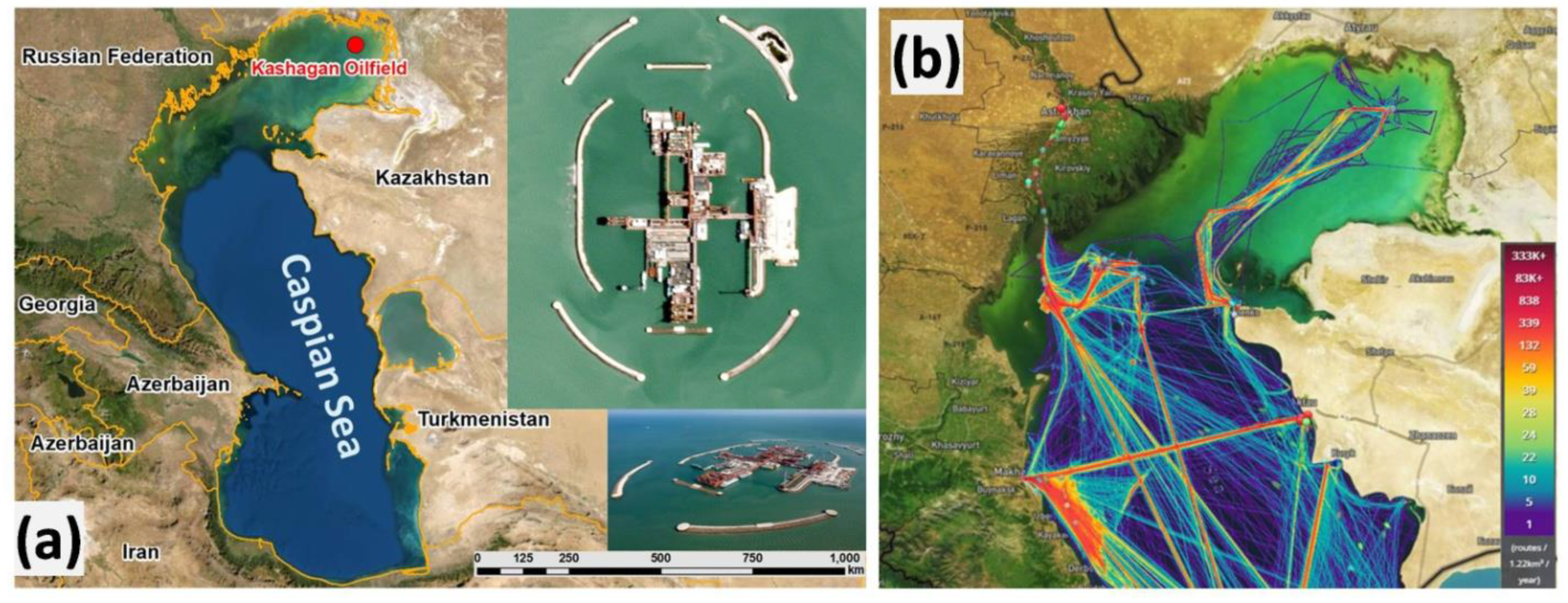
Kashagan is the offshore oilfield discovered in 2000 in Kazakhstan’s section of the Caspian Sea [
19]. The field is located in the northern part of the Caspian Sea (
Figure 1a). It is considered the world’s largest oil discovery in the last 30 years [
20] and is the first large-scale offshore petroleum development in Kazakhstan. Kashagan oilfield is located 4.2 km beneath the seabed, with an oil column extending over 1 km. It is a highly pressurized reservoir (800 bars and hydrogen sulfide around 16–20%) and is estimated to contain more than 35 billion barrels of oil with recoverable reserves of about 13 billion barrels.
Kashagan oilfield, operating since 2013, was selected as the study area for this research because it is one of the largest and most operationally difficult fields under extreme continental climate with cold winters and hot summers (air temperature ranging from −40 °C + 40 °C), temperature variations, ice cover with five-month duration (ice thickness reaching approximately 0.6–0.7 m), and intensive winds, currents and waves, and sea level fluctuations. The combination of these factors represents significant logistical and operational challenges for the heavy marine logistics and petroleum and gas industries (
Figure 1b).
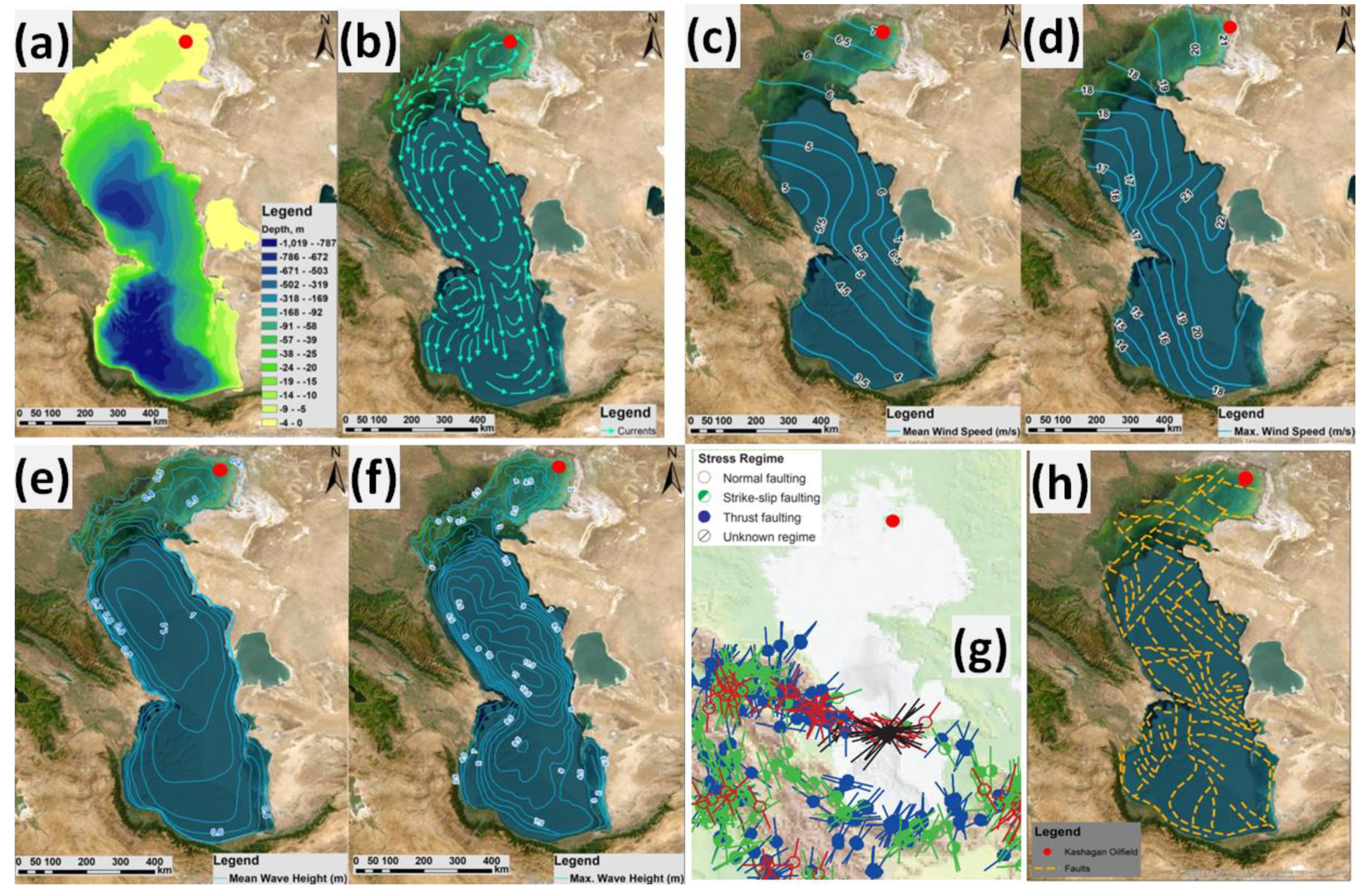
The oilfield is located in shallow water with a depth of 3–4 m (
Figure 2a). However, it is subject to regular sea-level fluctuations in the range of one meter. Current trends of lowering water levels in the Caspian Sea due to climate changes threaten the operations of the Kashagan oilfield, in particular, because of vessel approach logistics and new projects with critical dredging activities. Since 2005, the level of the Caspian Sea has dropped upto 1 m, and this falling tendency is still observed [
21]. The average sea level of the North Caspian is around −28.30 m.
Currents in the Caspian Sea are primarily wind-induced, with wind speeds and directions being the major shaping factors [
22,
23,
24,
25]. The shape and topography of the seashore and seabed of the Caspian Sea also exert a substantial influence on the currents [
26]. The typical current speed value for the northern part of the Caspian Sea varies from 15 to 20 cm/s upto 30–90 cm/s [
27]. As seen in
Figure 2b, currents adapted from Lednev et al. [
22] show circulating patterns in the northern, central, and southern parts of the Caspian Sea. Similar spatial patterns of currents are obviously challenging for new projects, operations, and emergent reactions to oil spills.
The plains of the Caspian Sea are formed by currents and wave disturbances from which emerge large accumulative ridges up to a dozen kilometers or surfaces with peaks and small sand-shell islands [
28]. The most important hydrodynamic factors are river inflow, currents, and waves facilitating the transfer, sorting, and distribution of sediments [
28]. Similar dynamic changes in the subsea plain also cause difficulties and safety-related risks in the regular logistics and operations for ongoing operations and new projects.
Based on the extracted wind speed contour lines from the studies by Rusu et al. [
29] in the northern part of the Caspian Sea, it was possible to observe the mean wind speed in the range of 6–7 m/sand maximum wind speed in the range of 18–21 m/s during the winter period of January 2001–December 2011 (
Figure 2c,d). As mentioned before, winds control the formation of currents with an approximate speed of several centimeters per second to 100 cm/s [
30].
Based on the extracted wave height contour lines from the studies by Myslenkov et al. [
31], it was possible to observe the mean wave height in the range of 0.2–0.5 m and maximum wave height in the range of 2–4.5 m/s during 1979–2017 (
Figure 2e,f). According to Bezrodnykh et al. [
30], no high waves are observed in the Northern Caspian Sea due to its shallowness and ice cover during the winter period.
Figure 2.
(
a) Bathymetry (based on GEBCO Gridded Bathymetry Data); (
b) currents of the Caspian Sea; (
c) mean and (
d) maximum wind speeds in the Caspian Sea; (
e) mean and (
f) maximum wave heights in the Caspian Sea; (
g) Caspian Sea region from World Stress Map 2016 by Heidbachet et al. [
32]; (
h) faults.
Based on the World Stress Map 2016 for the Caspian Sea region by Heidbach et al. [
32], the northern part is not seismically active (
Figure 2g). Therefore, it was not possible to relate detected subsidence hotspots to any kind of seismic processes. Additionally, recent studies by Bayramov et al. [
33] showed that the closest Tengiz oilfield at the coast of the Caspian Sea was subsiding because of man-made oil extraction and injection activities rather than seismicity. Based on the map of the Caspian Sea faults adapted from Levin et al. [
34], it was possible to observe that the Kashagan Field is located near a fault that might be subject to possible future activations either because of tectonic and seismic processes or man-made extraction of oil and gas resources (
Figure 2h).
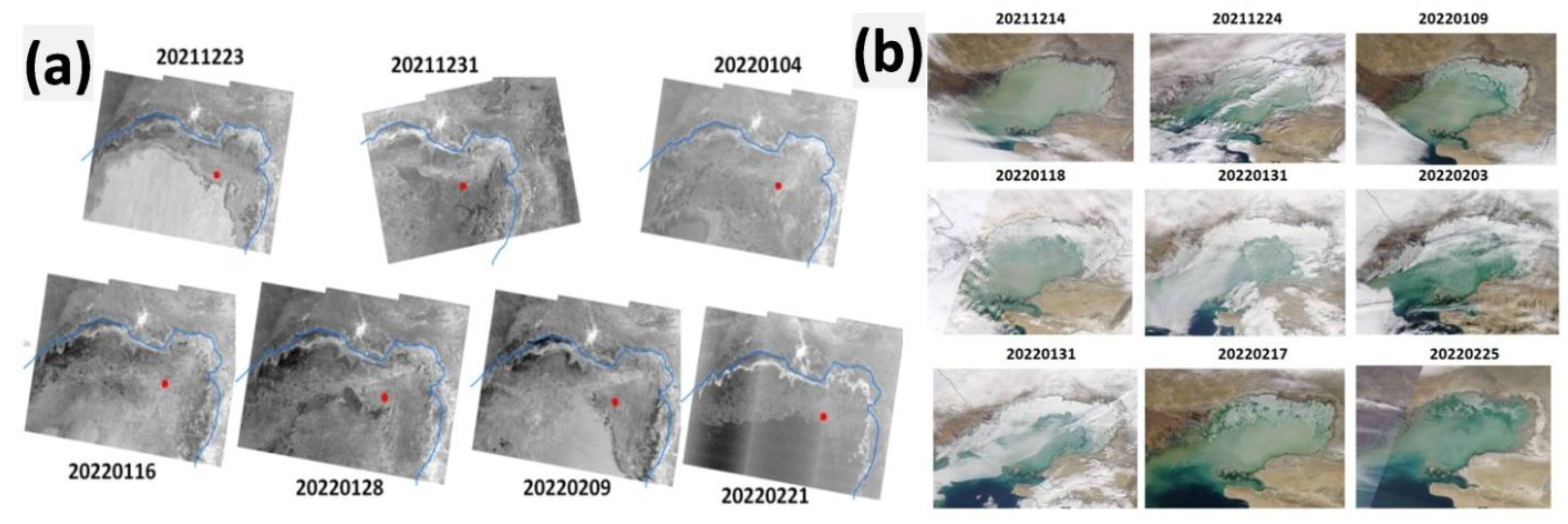
The Kashagan oilfield was developed on artificial islands with ice-protection barrier structures (
Figure 1a). Winters are harsh, and air temperatures can drop to −40 °C. The summer temperatures can reach +40 °C. The sea waters are normally frozen from November to March, with an average ice thickness of about 60–70 cm. Interpretation of recent time-series Sentinel-1 radar in
Figure 3a and MODIS Terra/Aqua optical satellite images in
Figure 3b showed that the Kashagan Field was mainly covered by ice during December 2021–February 2022. According to Bezrodnykh et al. [
30], complete ice melting occurs at the end of March–beginning of April. The ice, shallow waters, sea level fluctuations, and high levels of hydrogen sulfide represent a significant logistical challenge in the Kashagan Field.
3. Data Processing
Quantitative Assessment of Kashagan Platform Surface Deformations Using PS-InSAR and 2D Decomposition for Vertical and Horizontal Movements
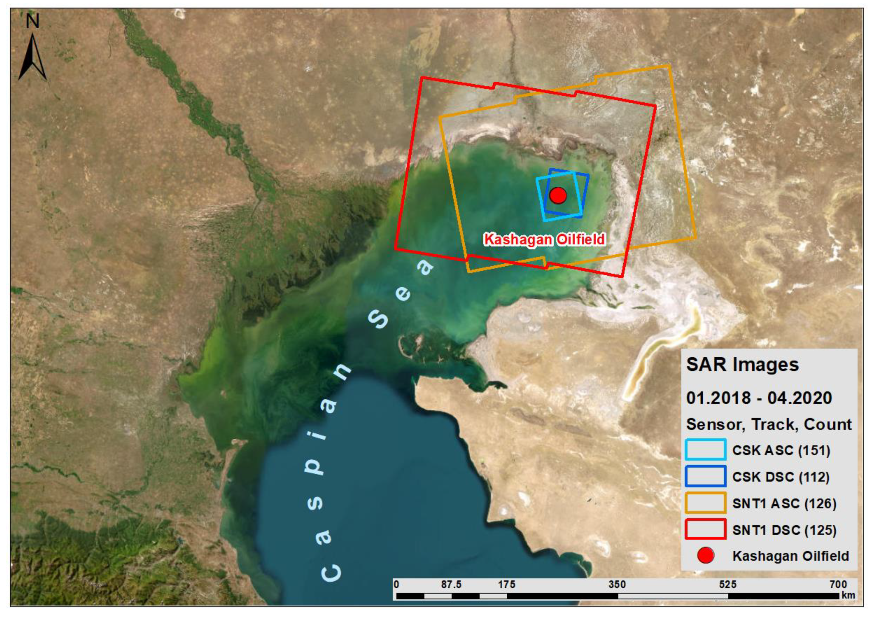
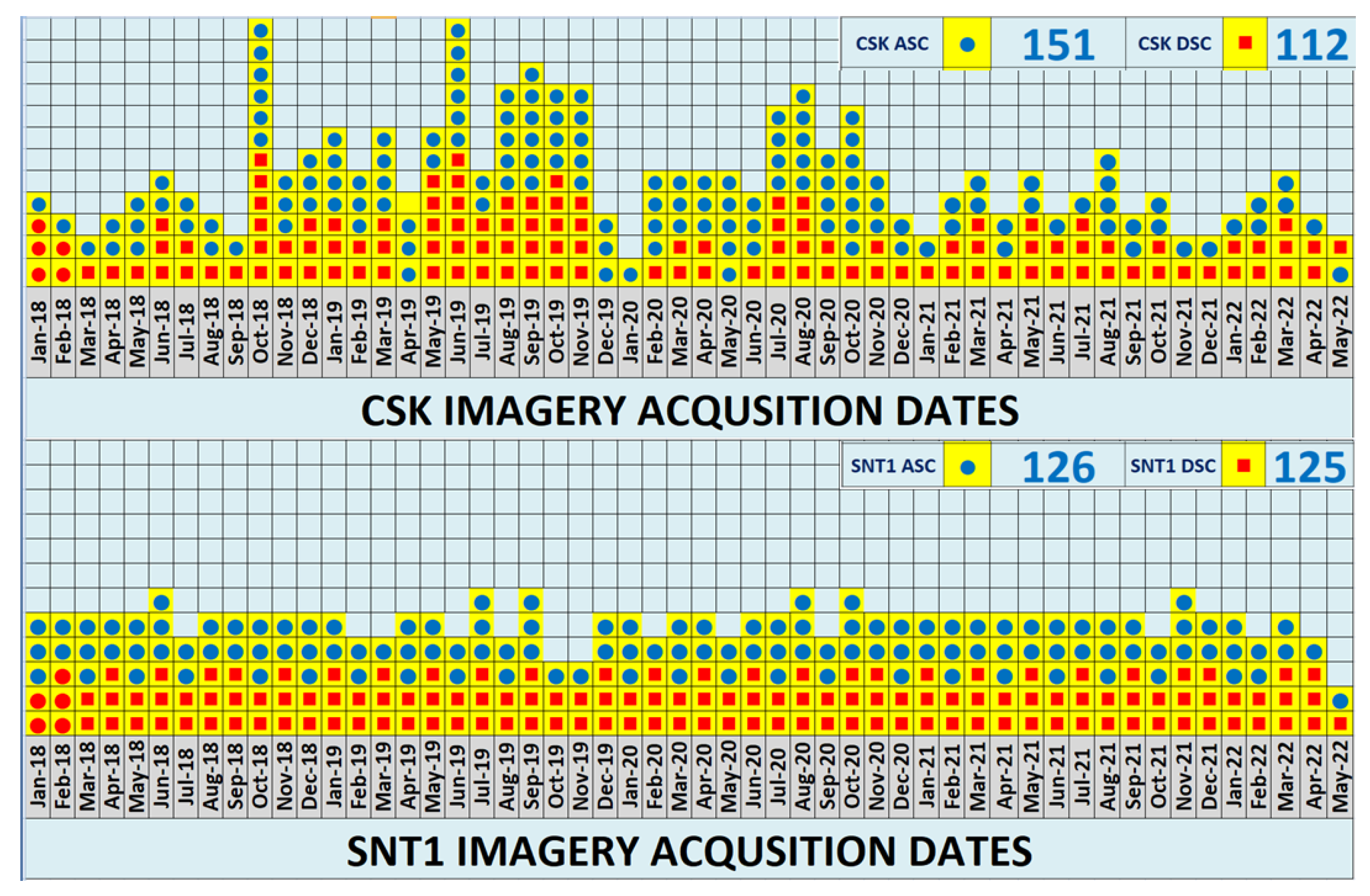
Monitoring and characterization of the Kashagan oilfield deformations have been carried out using interferometric stacks of SNT1 and CSK SAR satellite images from the European Space Agency (ESA) and the Italian Space Agency (ASI) (
Table 1). The satellite observations covered the period January 2018–May 2022. Even though SNT1 held longer temporal coverage of observations, starting from 2015, in the framework of this study, it was decided to focus on the common observation period of SNT1 and CSK that was constrained by the availability of the CSK dataset. This choice was needed to perform a cross-validation of the obtained results. The footprint of the SNT1 and CSK frames are presented in
Figure 4. The line plot of the count of images by acquisition dates is presented in
Figure 5. This graph presents that all SAR images were well connected in time in order to follow the differential vertical and horizontal displacement monitoring over the period of 2018–2022. The characteristics of both satellite missions are presented in
Table 1. VV and HH polarizations of SNT1 and CSK, respectively, were used due to the proven higher coherence of co-polarized acquisitions in the case of deformation monitoring applications [
33,
35]. SNT1 and CSK imagery were acquired from both descending (DSC) and ascending (ASC) tracks, allowing to derive differential vertical and horizontal deformation velocities and cumulative deformations using 2D decomposition of LOS measurements.
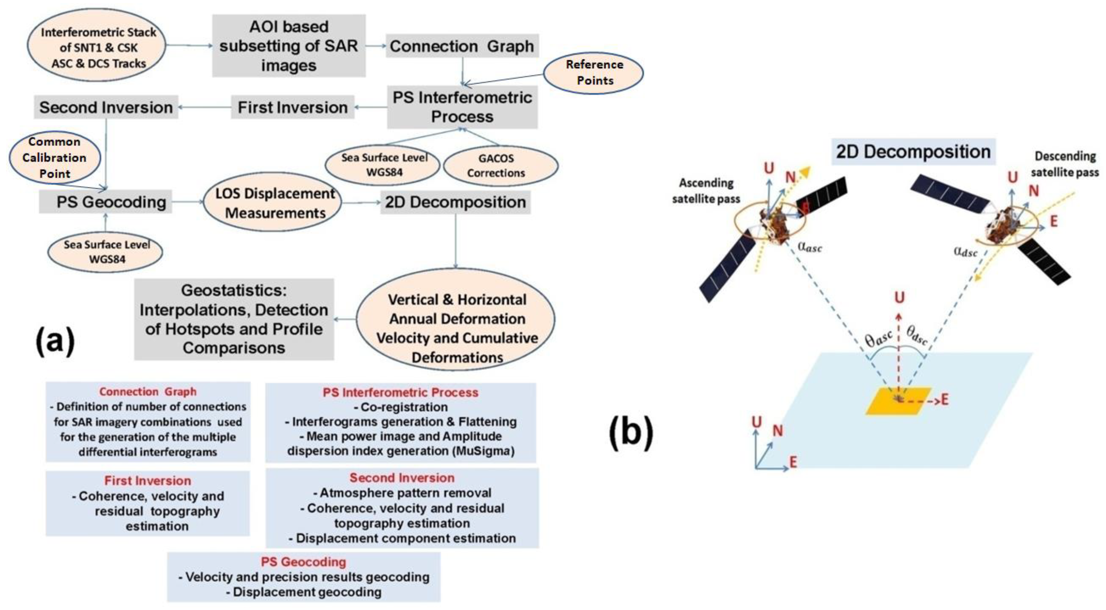
The CSK and SNT1 SAR images were processed using the PS-InSAR technique in the ENVI SARscape software version 5.6.2 with the processing workflow presented in
Figure 6a and the principle in
Figure 6b [
36]. PS-InSAR is a proven single-reference technique (N interferograms with N + 1 SLCs) for the processing to measure persistently reflecting surface features and their motion rates with high precision [
18,
37]. On artificial surfaces, such as oil and gas infrastructure, PS-InSAR is generally expected to maintain high coherence [
37]. Three main processing stages were performed for this research: PS-InSAR, 2D decomposition of line-of-sight (LOS) measurements from ascending and descending tracks, and geostatistical analysis. The PS-InSAR processing consisted of interferogram generation, multi-temporal persistent scatterers processing, and removal of atmospheric phase screen [
38].
PS-InSAR measures deformation projection along the LOS direction for DSC and ASC tracks. Ascending and descending LOS deformations can be decomposed along the vertical and horizontal (east–west) directions [
39,
40]. LOS velocities derived from ASC and DSC tracks of SNT1 and CSK images were separately decomposed into the horizontal component along the east-west direction
dhor and the vertical component
dver taking into account the local incidence angle of the satellite view by Equation (1) [
41,
42,
43,
44,
45,
46,
47].
where
asc and
dsc are the local incidence angles, and
asc and
dsc are the satellite heading angles of the ASC and DSC modes, respectively [
48,
49].
Figure 6.
(
a) PS-InSAR workflow; (
b) 2D decomposition principle adapted from Fuhrmann et al. [
49].
Figure 6.
(
a) PS-InSAR workflow; (
b) 2D decomposition principle adapted from Fuhrmann et al. [
49].
The natural-neighbor interpolation method with a spatial resolution of 0.5 m was used for the generation of differential vertical and horizontal deformation surfaces to detect subsidence and uplift hotspots in the Kashagan oilfield. The natural-neighbor method showed better interpolation and visualization performance in comparison to inverse distance weighting (IDW) and Kriging interpolation methods. Further geospatial analytics were performed for the comparative analyses between PS-InSAR measurements derived from SNT1 and CSK images.
The following steps were performed in the ENVI SARscape PS-InSAR processing chain: 1. connection graph; 2. interferometric process; 3. first inversion step; 4. second inversion step; 5. geocoding; 6. 2D decomposition [
36]. The connection graph functionality defined the SAR pair combinations and connection network for the generation of the multiple differential interferograms. The interferometric process step allowed us to automatically process the coregistration and the interferogram generation. The first model inversion allowed us to derive displacement velocity and residual height without removing any phase component due to the atmosphere. The second inversion used the results of the first inversion to estimate the atmospheric phase components. The geocoding stage allowed the transfer of PS-InSAR slant measurements to geographic coordinates. Displacement decomposition allowed the calculation of the vertical and east–west components of the displacement [
36]. Further on, geostatistical interpolation was used to produce point density and displacement hotspot grids.
Measurements of surface displacements through interferometric techniques are affected by some limitations, such as spatio-temporal decorrelation related to the large perpendicular and long temporal baselines between SAR images and atmospheric phase delays [
50]. Since the Kashagan oilfield is located in the offshore environment, atmospheric artifacts often cause atmospheric phase delays, topographic uncertainty, and double-bounce effects from water (ice) surface, winds, and waves (
Figure 2a–f and
Figure 3a,b). It is also necessary to emphasize the factor of platform thermal expansion since it is being operated under extreme weather conditions, with temperatures dropping upto −40 °C.
However, PS-InSAR deployed within ENVI SARscape software allowed us, to the extent possible, to overcome those limitations on the interferometric processing stage with the integration of GACOS tropospheric delay maps downloaded from the Generic Atmospheric Correction Online Service for InSAR (GACOS) for the acquisition dates and time of SAR imagery [
51,
52,
53].
GACOS is computed based on the iterative tropospheric decomposition (ITD) model from Yu et al. [
51]. High spatial resolution zenith total delay maps are generated through the separation of stratified and turbulent signals from tropospheric total delays to be used for the correction of InSAR measurements [
51,
52,
53]. Datasets used in GACOS include the high-resolution ECMWF weather model at 0.1-degree and 6 h resolutions, SRTM DEM (90 m), and ASTER GDEM (90 m) [
51,
52,
53]. The resolution of the GACOS atmospheric correction grid was 90 m.
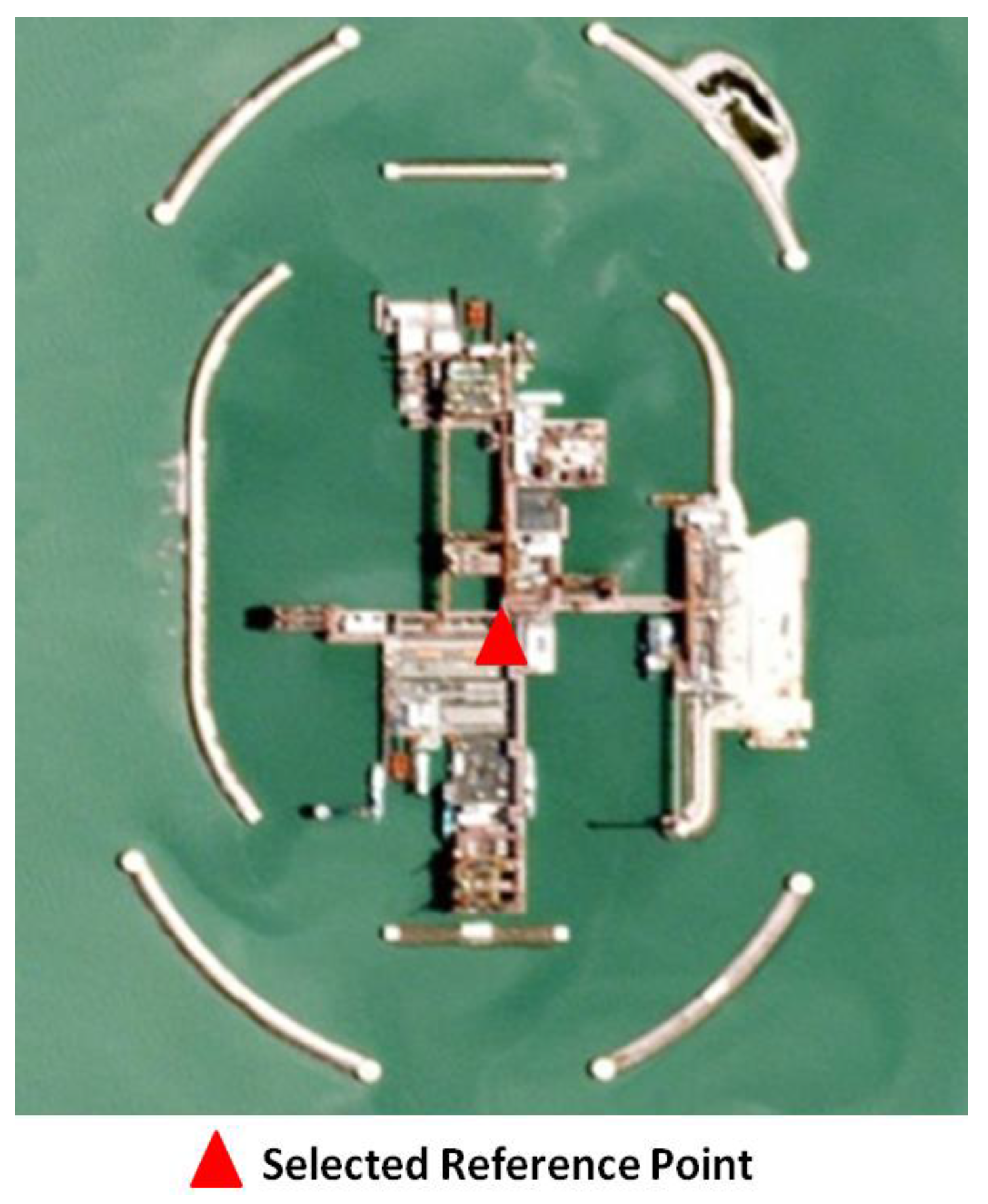
In the present studies, InSAR results were based on the relative or differential local measurements since neither short-term nor long-term geodetic measurements were available on the platform. Therefore, we selected one reference or spatial point on the oilfield and used it as an input ground control point (GCP) for the interferometric process stage (
Figure 6a and
Figure 7). This challenge poses a limitation since all measurements are considered relative or differential. It is obvious that we were not able to judge either the long-term displacement rates affecting the whole platform or the annual oscillations linked to temperature variations, wind speeds, and currents.
It is also necessary to emphasize that this platform is built on an artificial island, which makes it different from other offshore platform types that are subject to permanent oscillations. Since we did not have any GPS measurements, we could not perform more than relative measurements from the radar satellites with the assumption that this platform is less vulnerable to permanent oscillations caused by natural (winds, currents, sea level fluctuations, temperature variations, sea ice, seismicity, and tectonics) and operational man-made factors.
For the correct 2D decomposition and matching of LOS measurements from descending and ascending tracks, the common calibration point was selected in the geocoded displacement products. A point buffer zone of 22 m was used to find identical common persistent scatterers from descending and ascending tracks. The topographic contribution to the radar phase was corrected in the interferometric process stage using an artificially generated digital elevation model of the Caspian Sea level in the World Geodetic System 1984 (WGS84) with the spatial resolution of 1 m for the coverage of the Kashagan oilfield. Unfortunately, there was no accessible digital elevation model of the Kashagan oilfield.
Since there were no accessible standards from the Kashagan oilfield to judge the criticality of measured displacements, we had to apply professional expert feedback from ten geotechnical engineers in Kazakhstan and also checked on any publicly announced deformation-related incidents.
4. Results
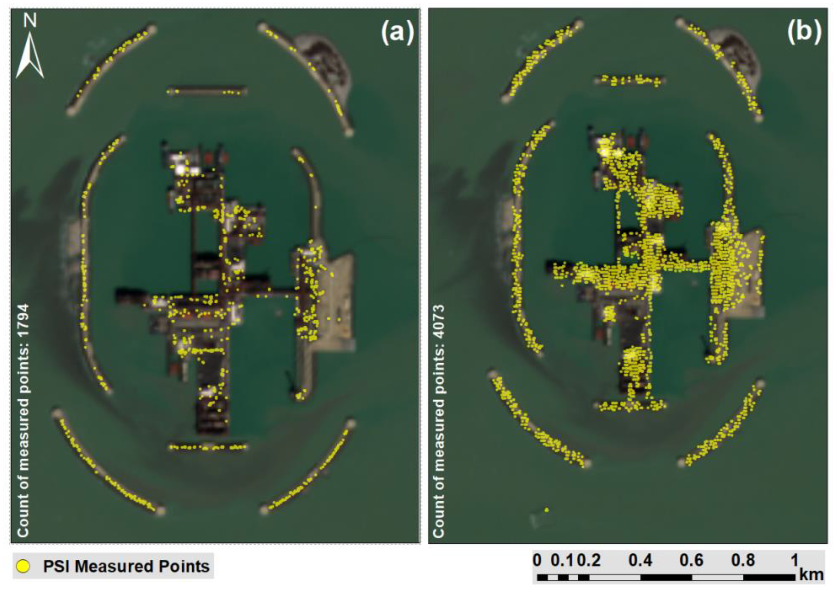
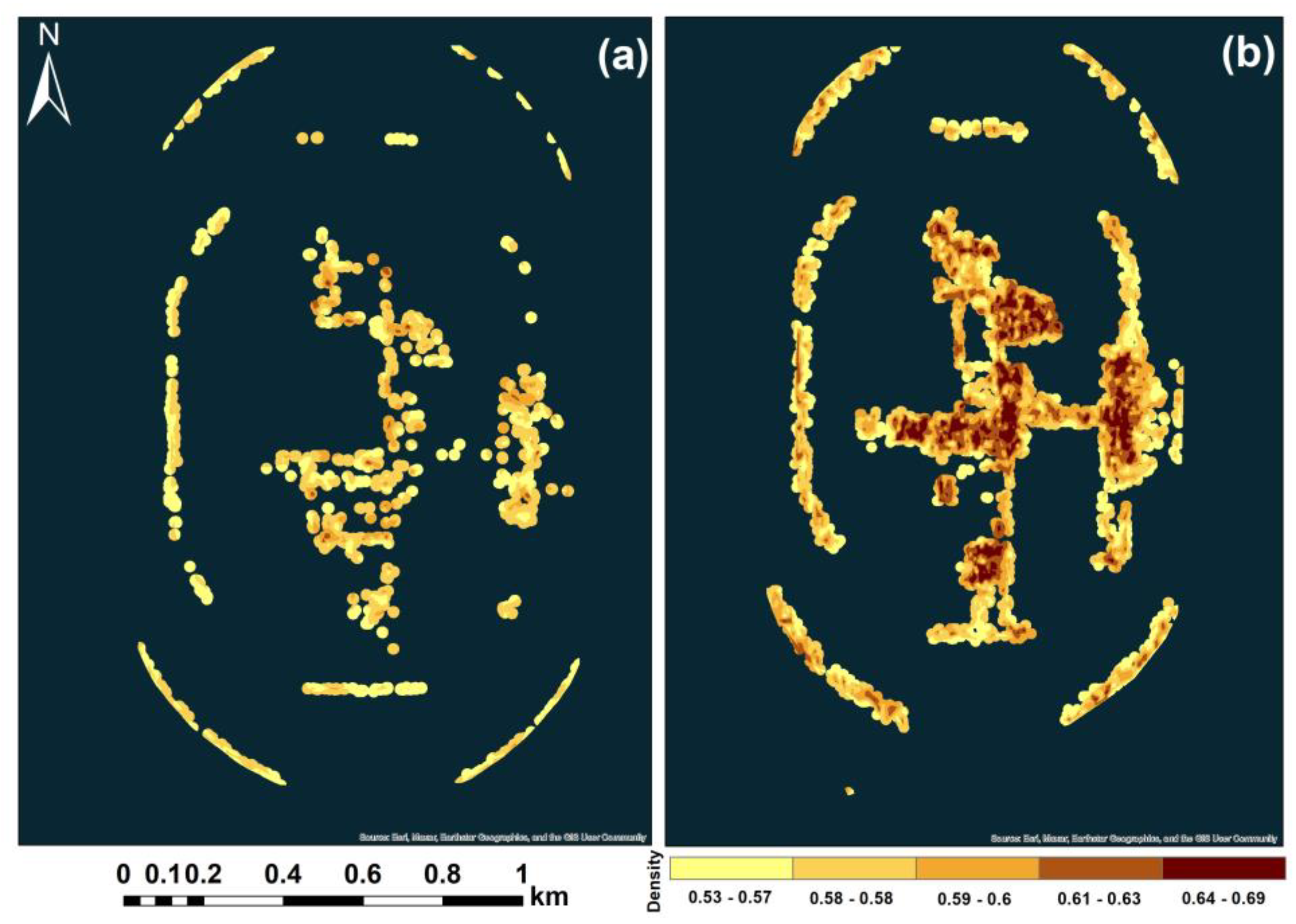
The counts of PS-InSAR-measured points were observed to be 1794 for CSK and 4073 for SNT1 images (
Figure 8a,b). The density of PS-InSAR measurements derived from SNT1 was higher compared to CSK (
Figure 8a,b). This was related to the multi-temporal coherence differences between SNT1 and CSK (
Figure 9a,b).
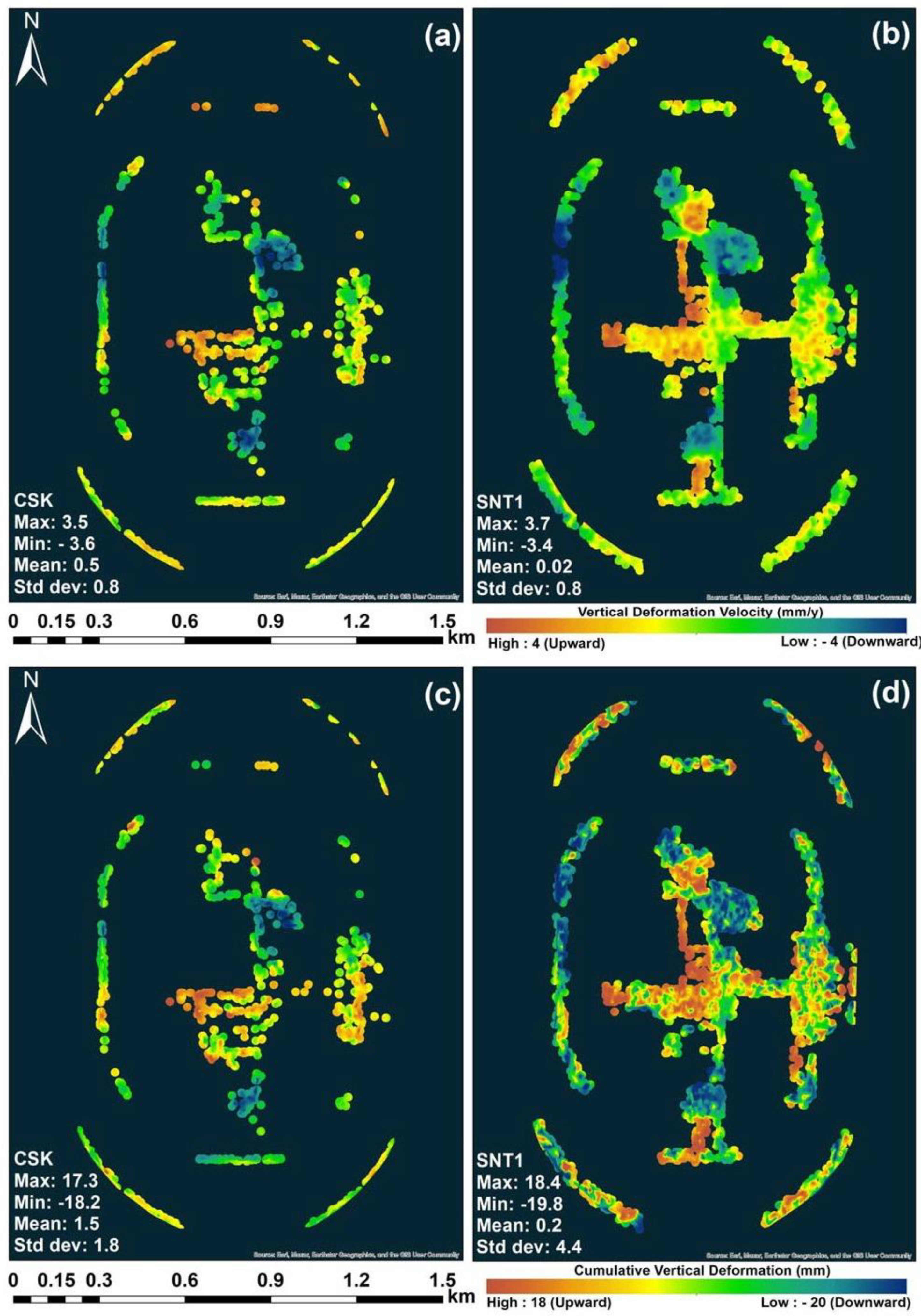
Differential VD derived from 2D decompositions of CSK ASC–DSC LOS and SNT1 ASC–DSC LOS measurements are presented in
Figure 10a,b. PS-InSAR differential vertical deformation measurements derived from CSK and SNT1 showed a good agreement in the spatial subsidence and uplift patterns (
Figure 10a,b). Differential vertical subsidence and uplift velocities for the Kashagan oilfield were observed to be between −4 mm/y and 4 mm/y from both CSK and SNT1 datasets from 9 January 2018 to 30 April 2022 (
Figure 10a,b). Differential cumulative vertical subsidence and uplift velocities for the Kashagan oilfield were observed to be between –20 mm/y and 18 mm/y from both CSK and SNT1 images from 9 January 2018 to 30 April 2022 (
Figure 10c,d). Even though the measured differential vertical velocities and cumulative displacements were not characterized by a dramatic deformation rate, it was possible to clearly observe the spatial variability related to subsidence and uplift hotspots in
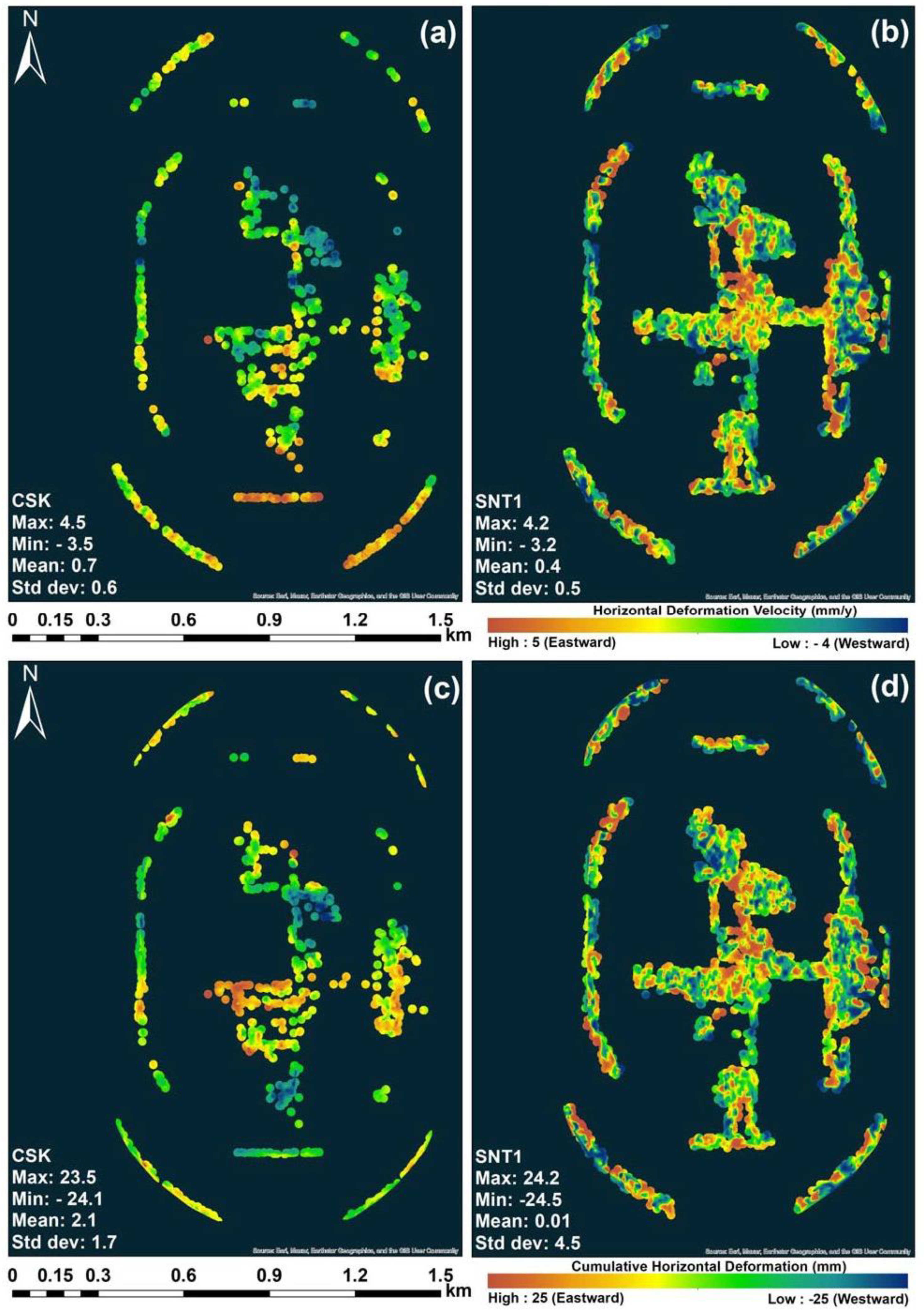
Figure 10a–d. Differential HD derived from 2D decompositions of CSK ASC–DSC LOS and SNT1 ASC–DSC LOS measurements are presented in
Figure 11a,b. PS-InSAR horizontal measurements derived from CSK and SNT1 images did not show identical spatial displacement patterns. Differential horizontal velocities for the Kashagan oilfield were observed to be between −4 mm/y and 5 mm/y for CSK and SNT1 images from 9 January 2018 to 30 April 2022 (
Figure 11a,b). Differential cumulative horizontal velocities for the Kashagan oilfield were observed to be between −25 mm/y and 25 mm/y from 9 January 2018 to 30 April 2022 (
Figure 11c,d).
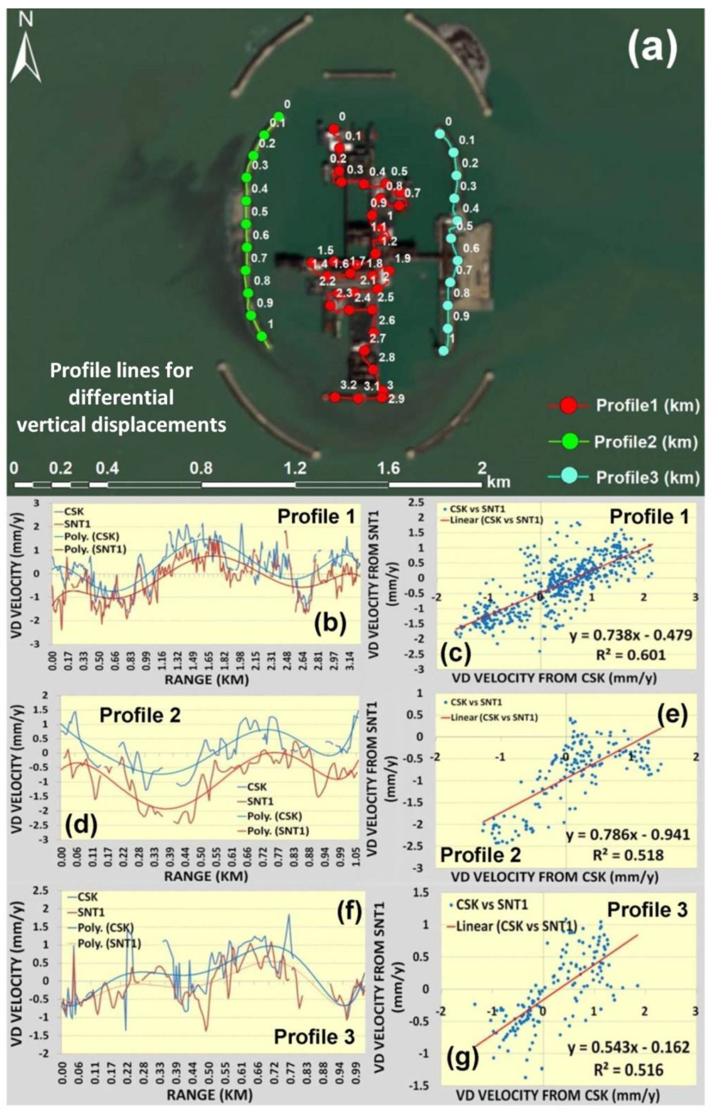
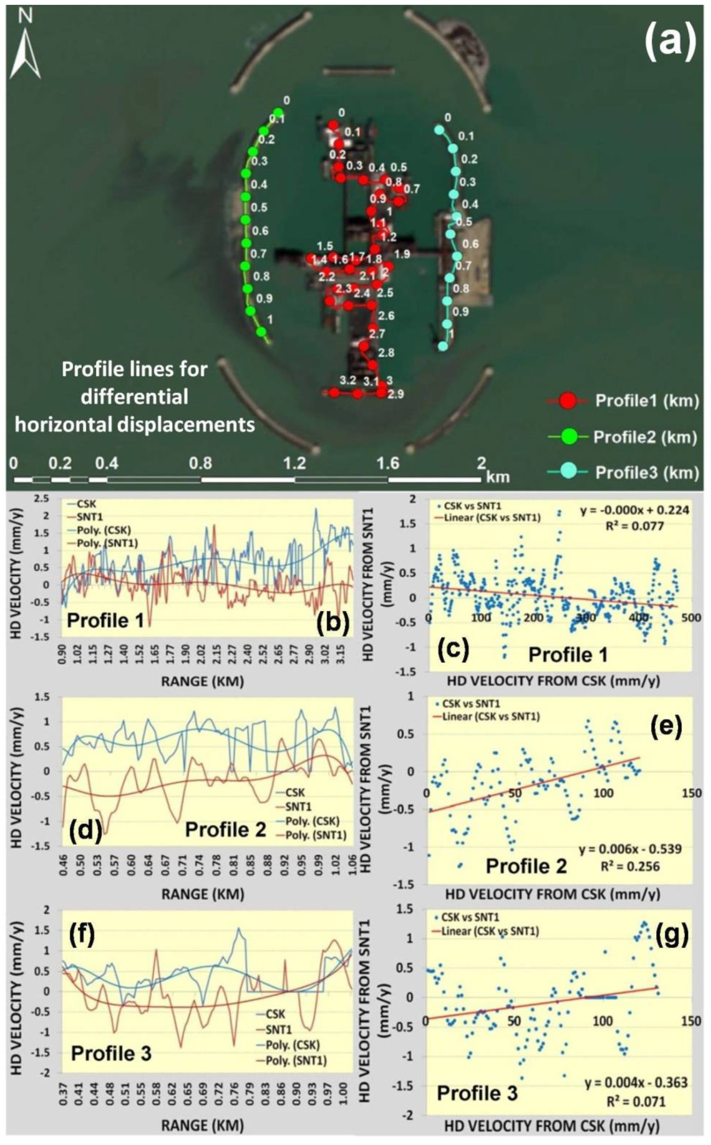
The comparison of differential VDs for three profile lines in
Figure 12a of the Kashagan oilfield showed a moderate agreement with identical polynomial trend lines and R
2 > 0.50 (
Figure 12b–g). Even though a common calibration point was used for PS-InSAR measurements, the observed systematic shift between the trendlines of SNT1 and CSK was observed to be in the range of 0.3 mm–2.4 mm (
Figure 12b,d). This shift could be caused by different natural and man-made factors, as well as the spatial resolutions of the SNT1 and CSK satellite missions affecting the processing quality. However, it is difficult to derive the particular reason because PS-InSAR accuracy is around ±1 mm. As mentioned before, we did not have historical geodetic measurements as a reference, and our PS-InSAR measurements were differential based on the selected reference point (
Figure 7).
The comparison of differential HDs for three profile lines of the Kashagan oilfield did not show identical spatial patterns with poor agreement of R
2 < 0.26. (
Figure 13a–g).
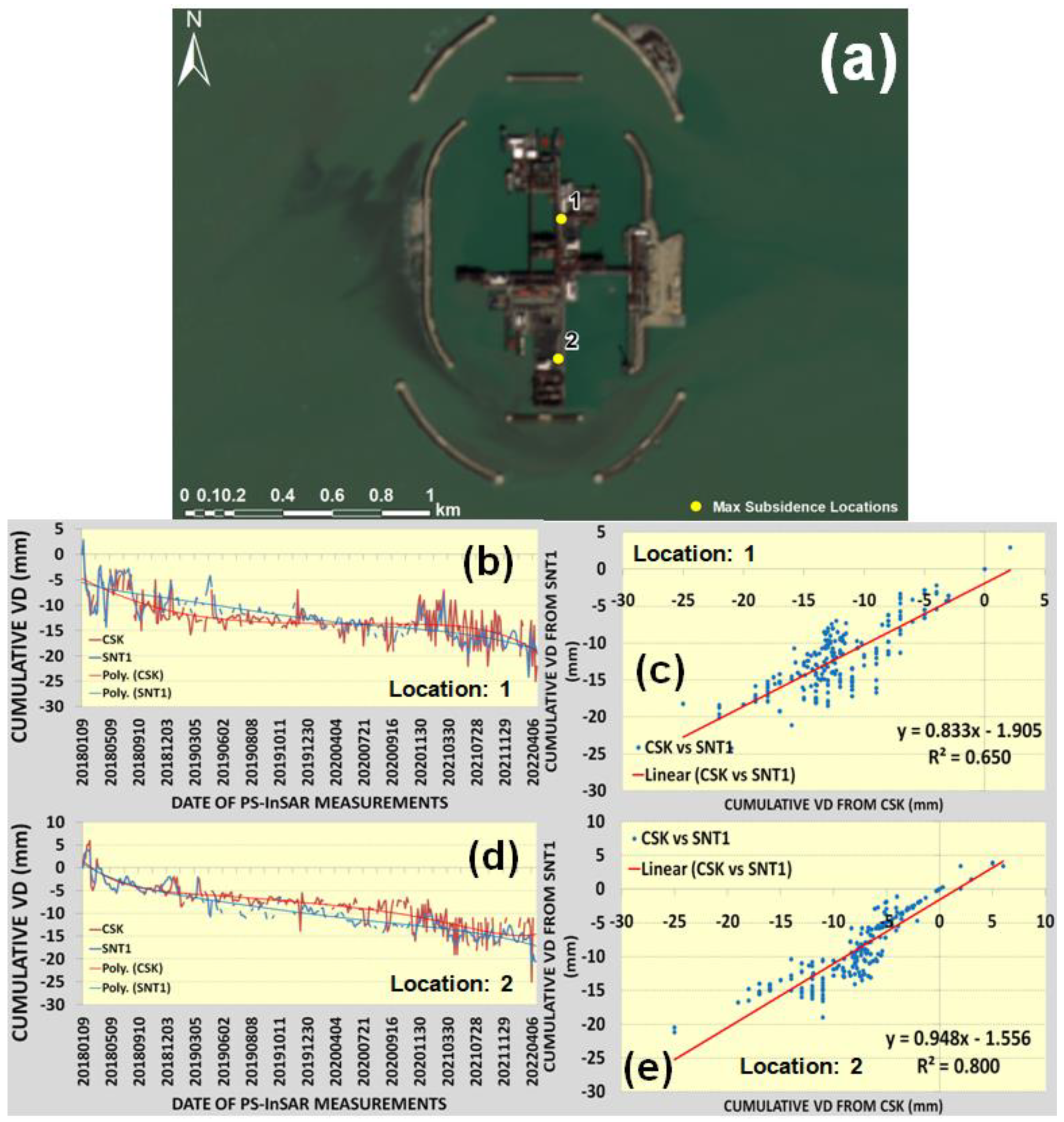
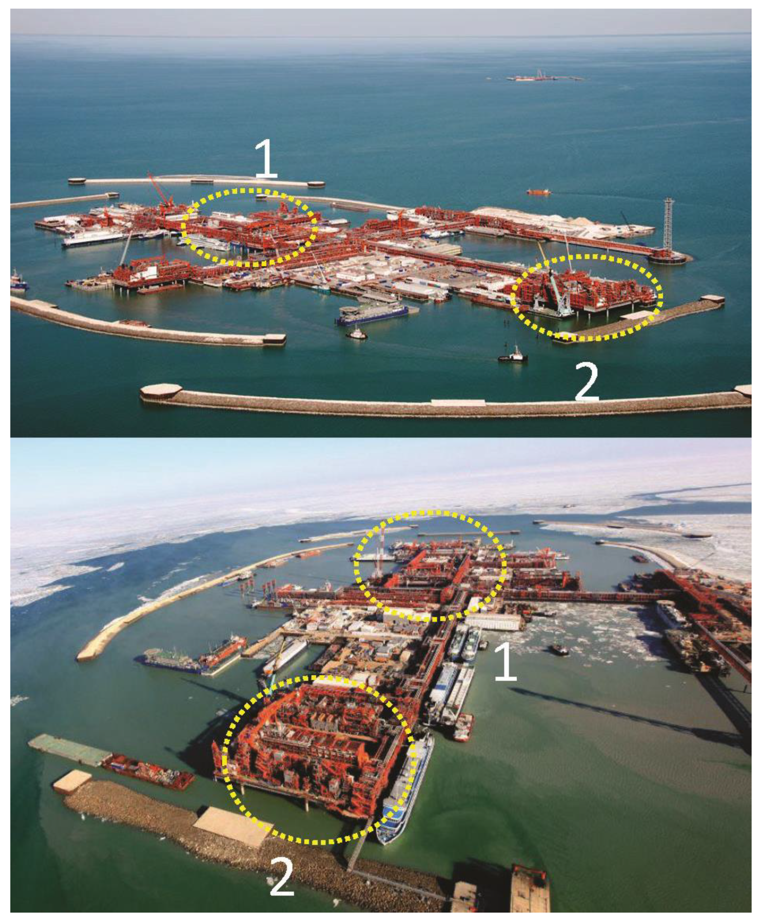
The maximum differential cumulative subsidence reaching around −20 in 2022 was observed for two locations presented in
Figure 14a. The regression analysis between differential cumulative displacements derived from CSK and SNT1 showed a moderate agreement with R
2 > 0.65 for both most subsiding locations (
Figure 14b–e). Based on
Figure 15 of the Kashagan oilfield, it was possible to determine that both of these detected hotspots were located at the oilfield areas installed on piles. This allowed us to assume that these areas were more vulnerable to movements caused by natural and anthropogenic factors.
5. Discussion
As a result of this research, it was possible to conclude that the differential vertical displacement velocities (−4 mm/y and 4 mm/y) and differential cumulative displacements (−20 mm/y and 18 mm/y) at the Kashagan oilfield are not intense, even though the offshore platform was operated since 2013 under extreme weather conditions in terms of winter temperatures and wind speeds, currents, waves, sea ice, and water level fluctuations in the Caspian Sea. However, we are only able to judge it based on the differential measurements, which are relative to our selected reference point on the oilfield. Since we did not have any long-term GPS measurements from the Kashagan Field, we are not able to conclude about either the entire oilfield displacements or regular oscillations caused by natural or man-made factors. We are well aware of this limitation for this study, but nowadays, it is beyond achievable since we experience a lack of critically needed time-series geodetic measurements from the Kashagan oilfield. Kashagan oilfield is built on an artificial island, which makes it different from other types of offshore platforms vulnerable to permanent oscillations. Based on this fact, we could assume that our PS-InSAR measurements are less affected by permanent oscillations caused by wind and currents. However, we could not judge the dynamic behavior of the oilfield caused by significant temperature variations and sea ice.
Even though detected differential vertical deformation velocities and cumulative deformation are not dramatic during the period of 2018–2022, the detected hotspots installed on piles could require future investigations in case the deformation trend is defined as non-compliant by engineering and geotechnical risk assessment standards for offshore platforms. Unfortunately, it was not possible to find some accessible engineering and geotechnical standards to understand what was considered critical criteria for the mitigation of vertical and horizontal displacement risks in marine conditions. The multi-temporal coherence of the PS-InSAR measurements derived from SNT1 was higher than from CSK. Higher temporal decorrelation of X-band CSK images in comparison to C-band SNT1 was also reported by Bayramov et al. [
33] and Morishita et al. [
54]. According to Morishita et al. [
54], one of the reasons why the coherence for the C-band is higher than the X-band is the lower resolution of the C-band. Higher decorrelation of CSK images is also explained by the higher frequencies of this satellite mission and, therefore, a higher sensitivity to small changes in the analyzed surfaces [
55,
56,
57]. The multi-temporal coherence range of 0.53–0.69 was expected to be higher from both SNT1 and CSK since the analysis is focused on a stable marine infrastructure built on artificial islands with ice protection structures. This range of coherence can be explained by the movement/vibration of the steel structures due to winds, currents, waves, and sea ice, as well as atmospheric phase delays caused by extreme weather conditions [
12].
PS-InSAR produced different spatial distributions and densities of measurements from CSK and SNT1 images. To improve the result geolocation and deformation precision, it is highly recommended to start permanent GPS observations for the stable points on the oilfield and also produce an accurate digital elevation model based on LIDAR or drone surveys. At the same time, one of the advantages of interferometric measurements is the wide spatial coverage of observations, which could allow prioritization of the most critical areas for the planning of detailed insitu geohazards risk management campaigns, installation of permanent GPS stations or the implementation of regular geodetic surveys. Based on the successful studies by Palano et al. [
58], GPS stations provided very high precision and reliability in the measurements of vertical and horizontal movements of offshore platforms. However, it is necessary to emphasize that specifically for Kashagan, the application of a high-precision geodetic approach with continuous GPS measurements could not provide a high density of measurements for the entire range of the oilfield as well as extended historical temporal coverage such as PS-InSAR.
PS-InSAR measurements of differential vertical velocity and differential cumulative displacements derived from CSK and SNT1 showed a moderate agreement with R2 > 0.50. PS-InSAR measurements of differential horizontal velocity and differential cumulative displacements derived from CSK and SNT1 showed poor agreement in terms of spatial patterns and R2 < 0.26. However, we could not validate the performance of CSK and SNT1 satellite missions for the measured differential horizontal displacements since we were lacking for the third satellite mission. On the other hand, this allowed us to assume that the Kashagan oilfield is more vulnerable to dynamic differential horizontal movements by direct natural factors like winds, currents, waves, sea level fluctuations, sea ice, and seismicity and also relating to the variations in measurements by different satellite missions.
As previously mentioned, to the extent of our awareness, similar studies have never been performed for the Kashagan oilfield using interferometric techniques as part of the research results accessible to the scientific community. Therefore, we plan to expand present studies with additional satellite missions and methods of interferometric measurements. Additionally, we plan to expand our studies by numerical simulations of PS-InSARmeasurements to make deformation predictions in the Kashagan oilfield [
59,
60].
Since we did not have any insitu reference points with long-term GPS measurements, the cross-validation of differential measurements was only possible based on the comparison of different medium-resolution and high-resolution satellite missions with sufficient descending and ascending acquisitions for the cross-validation of PS-InSAR measurements in this study. Accordingly, it is planned to deploy other interferometric techniques assigned for the deformation monitoring of man-made structural stability as well as to extend the observation period.
6. Conclusions
The differential vertical displacement velocity was observed to be between −4 mm/y (subsidence) and 4 mm/y (uplift), and the horizontal displacement velocity was observed to be between −4 mm/y (westward) and 5 mm/y (eastward)during 2018–2022 in the Kashagan oilfield. However, it was possible to observe the spatial patterns with the subsidence hotspots reaching differential cumulative displacement of −20 mm from both satellite missions—SNT1 and CSK.
The differential vertical displacement velocity and differential cumulative displacements derived from CSK and SNT1 images using PS-InSAR processing methodology showed identical spatial patterns with a moderate agreement of R2 > 0.50. Differences in the wavelengths, frequencies, and spatial resolutions of C-band SNT1 and X-band CSK missions were reflected in the variations in multi-temporal coherence and produced point density by the PS-InSAR measurements. Higher multi-temporal decorrelation of the CSK satellite mission was reflected in a lower point density than SNT1. The differential horizontal displacement velocity and differential cumulative displacements derived from CSK and SNT1 images using PS-InSAR processing methodology did not show identical spatial patterns with poor agreement of R2 < 0.26. It was not possible to ensure the quality of measured differential horizontal displacements since the research was lacking for the third satellite mission. On the other hand, this allowed us to assume that the Kashagan oilfield is more vulnerable to dynamic horizontal movements than vertical by natural factors such as winds, currents, waves, sea level fluctuations, sea ice, and seismicity. Another reason could be related to the atmospheric phase delays, which were, to the extent possible, eliminated using coarse-resolution GACOS corrections.
Based on the differential PS-InSAR measurements during 2018–2022, it was possible to assume that the Kashagan oilfield was not so vulnerable to natural (wind, currents, waves, sea ice, sea level fluctuations, and seismicity) and anthropogenic factors which could cause deformations. However, since we did not have any long-term GPS measurements from the Kashagan oilfield, we were not able to conclude about either the entire oilfield displacements or regular oscillations caused by natural or man-made factors.
Since engineering and geotechnical standards vary in what should be accepted as a critical level of subsidence or uplift depending on the type of marine and onshore petroleum and gas infrastructure, the risk assessment is subject to site verifications for the detection of any existing or potential damages. To prioritize vulnerable areas for site inspection activities and the planning of risk mitigation measures, interferometric technologies could play a significant role for petroleum and gas operators in onshore and offshore conditions.
The role of interferometric technologies is irreplaceable and advantageous because of wide-coverage measurements compared to standard geodetic measurements for selected positions, which are proven to be high precision. However, for the prioritization of locations to be continuously monitored by geodetic stations at subsidence or uplift hotspots, the role of the interferometric approach is crucial to effectively invest in the site measurement campaigns or evaluate whether it is worthwhile and reasonable to make investments from the risk assessment point of view.


