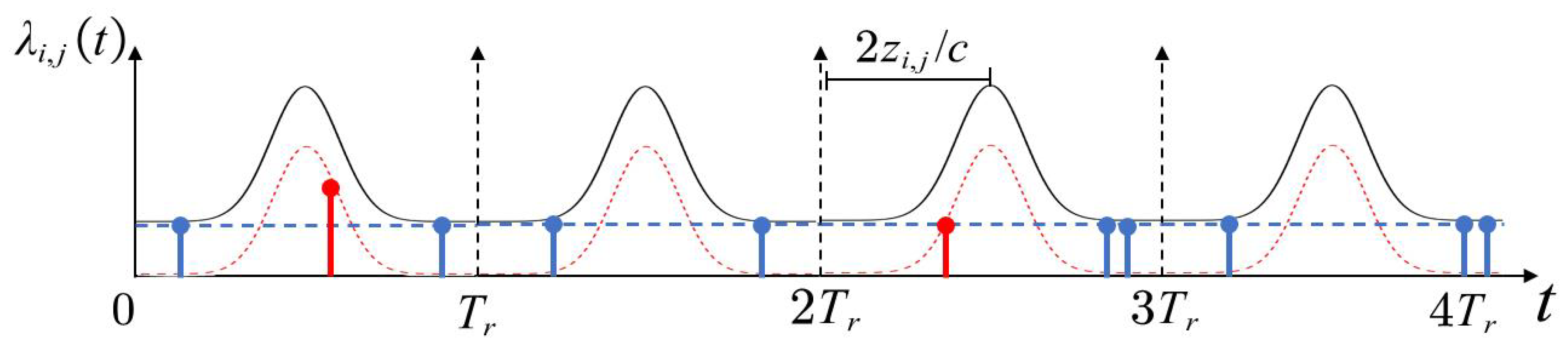
Figure 1.
Echo photon data observation model. Here, we show the generation process of echo photon data in four pulse detection cycles when there is only one target to be measured. When the first and third pulses are emitted, a signal count (red) is generated, and noise counts (blue) are generated after each pulse is emitted. (The red dashed line represents the signal response, the blue dashed line represents the noise response, and the black solid line represents the combined response.)
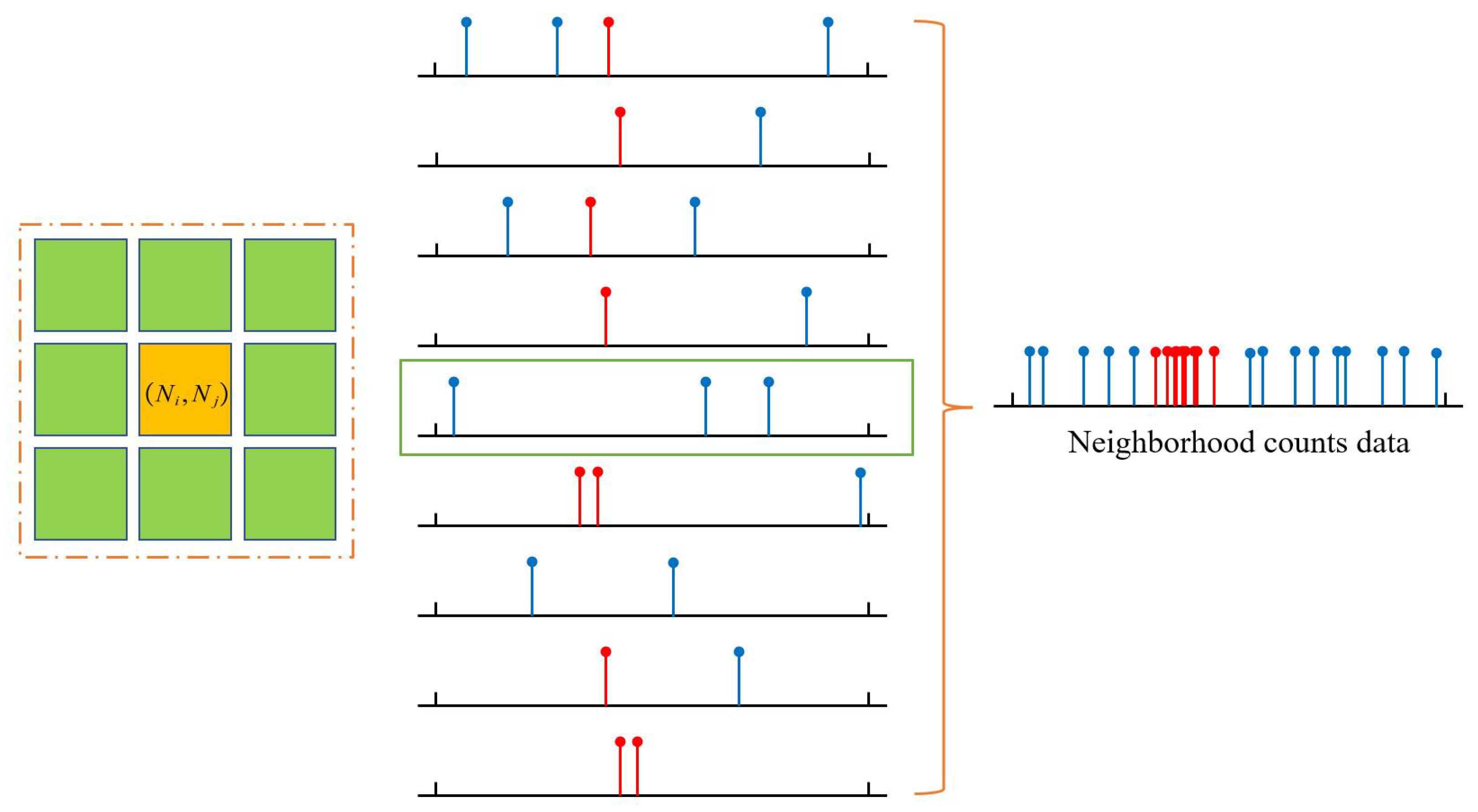
Figure 2.
Space sampling schematic diagram of photon counts. When there is no signal count in the echo photon data of the pixel , the count data of its 3 × 3 neighborhood pixels can be used to form a new dataset, which is helpful in solving the time range of the signal counts of the pixel (The red dashed line represents the signal response and the blue dashed line represents the noise response).
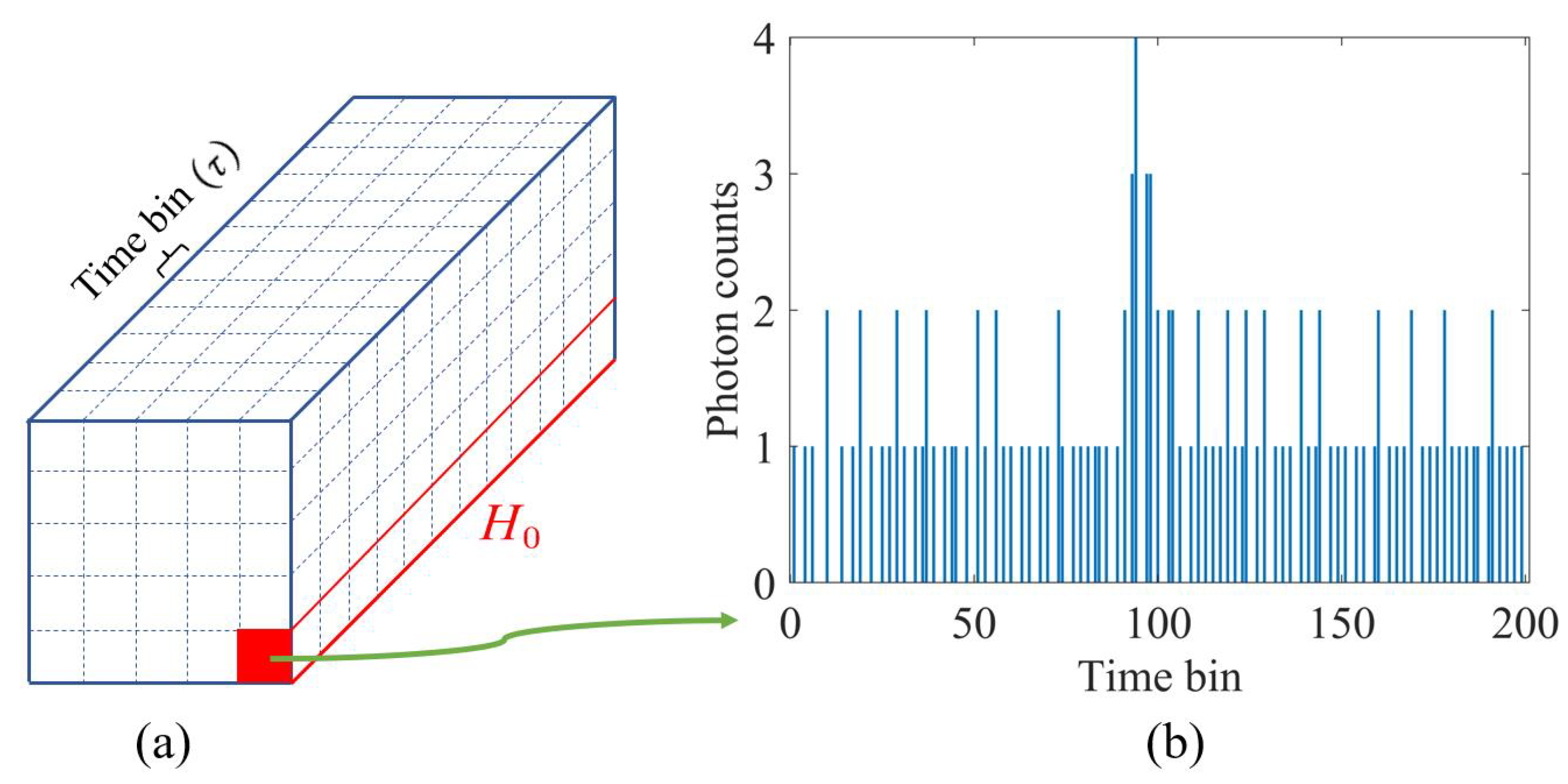
Figure 3.
Three-dimensional echo photon data schematic diagram. (a) The 3D echo data cube is composed of all pixels of the whole image when the time resolution is . (b) Photon statistical histogram of a single pixel in the cube, where the horizontal axis represents the position information of the time bin and the vertical axis represents the number of photons in each time bin.
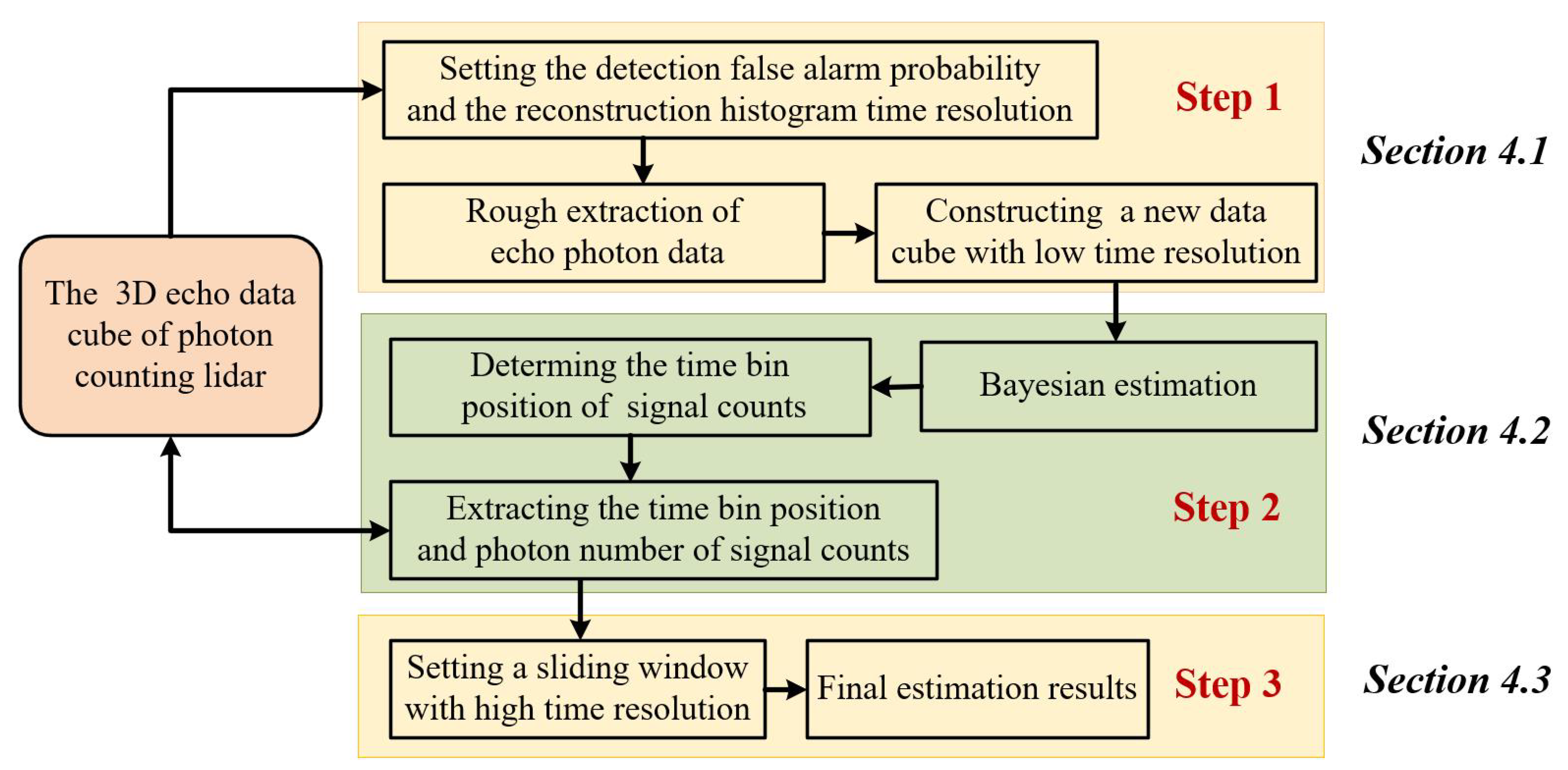
Figure 4.
Framework of our proposed method.
Figure 4.
Framework of our proposed method.
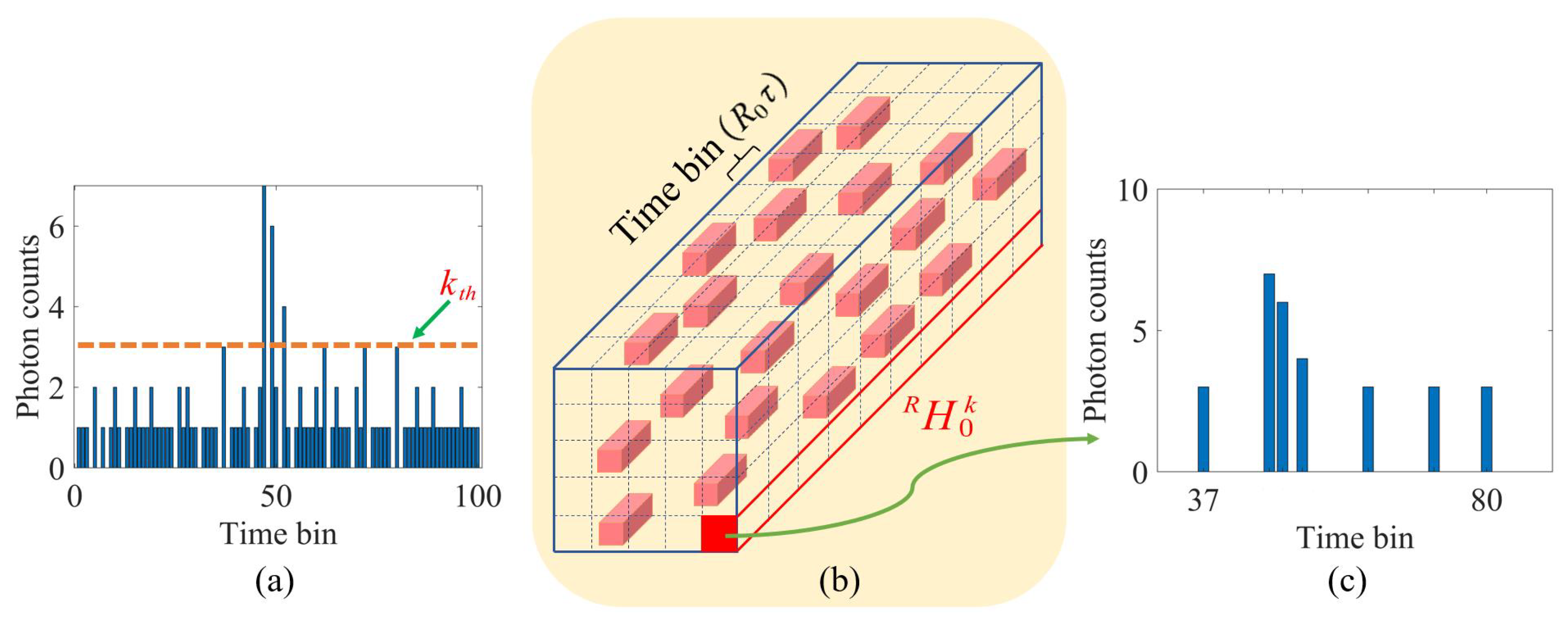
Figure 5.
Photon counting data extraction process under constant false-alarm probability. (a) The reconstructed histogram with a time resolution of . (b) The new cube data with a time resolution of obtained by constant false-alarm detection. (c) Subhistogram of a single pixel in the new cube composed of photon counts higher than the signal recognition threshold ().
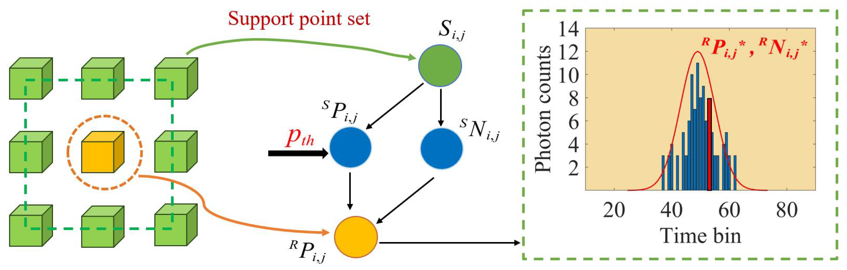
Figure 6.
The overall architecture of the Bayesian estimation method. When the support point set () is known, the preset time bin position detection threshold () is used to determine the position of the time bin where the signal photon cluster is located. Then, it is judged whether the photon counts at this position and the photon data of satisfy the Poisson distribution so as to obtain the time bin position () and the corresponding photon number () of pixel that satisfy the Bayesian model.
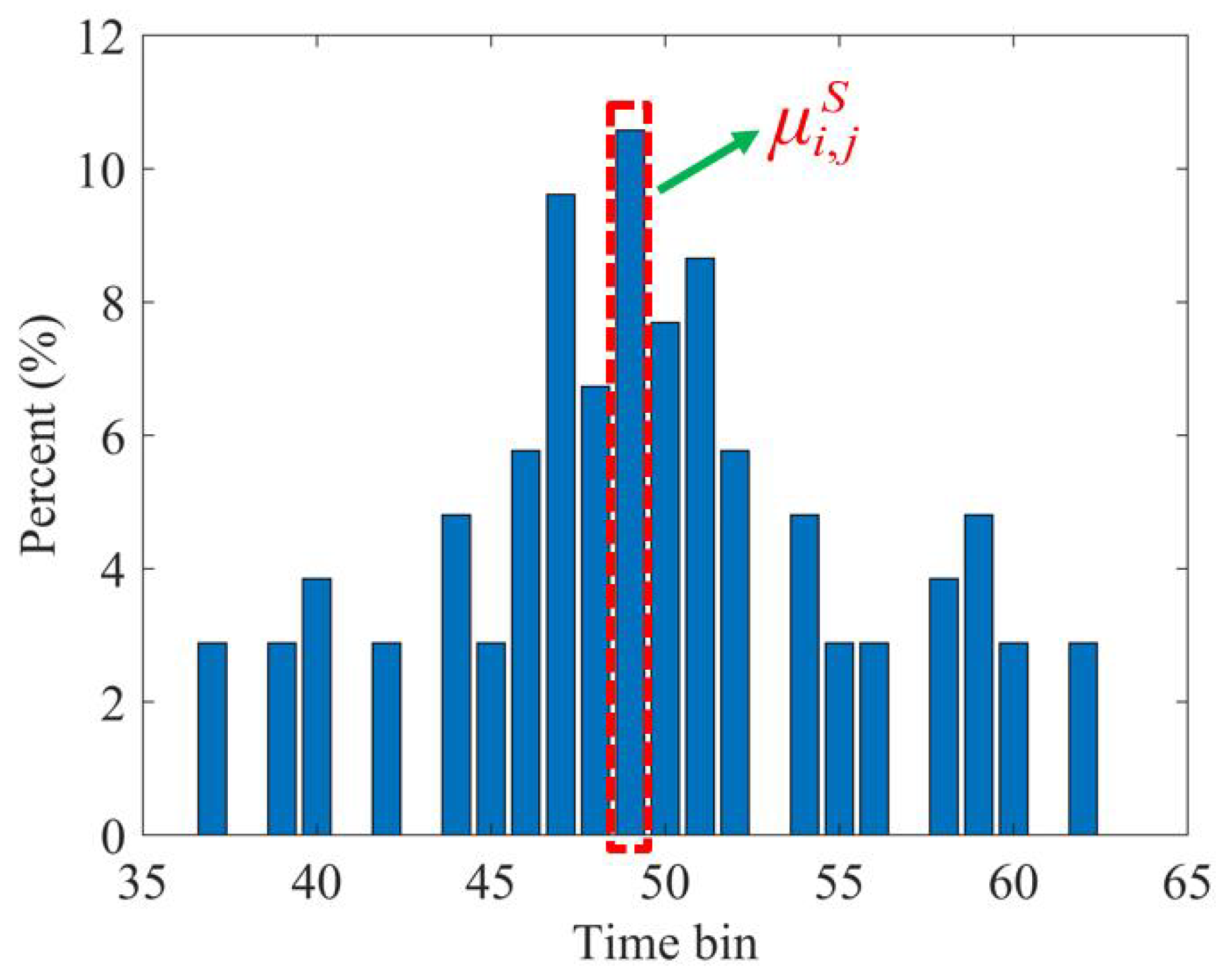
Figure 7.
The selection diagram of the Gaussian distribution mean (). The time bin position () of the echo photon data in the support point set () is accumulated into the same coordinate system, and the time bin position with the most occurrences is selected as the Gaussian distribution mean. The horizontal axis represents the position of the time bin, and the vertical axis represents the proportion of the position of each time bin.
Figure 8.
Discriminant diagram of the Poisson distribution to judge whether the photon number () corresponding to the result obtained under the prior condition and the photon number () in the support point set () satisfy the Poisson distribution. The distribution of the photon counts that conform (green) and do not conform (red) to Poisson distribution in the histogram is shown.
Figure 9.
The extraction of “empty” pixel photon count data and the sliding window diagram. (a) The 3D echo data cube composed of pixel and its 3 × 3 support point set after Bayesian estimation. (b) The number of signal counts of each pixel in the support point set. (c) The time interval of the signal counts in (b) when the time resolution is . We extract the photon count data in this time interval in the 3D echo data cube with a time resolution of and use a sliding window to slide through all the extracted data in turn.
Figure 10.
Undulating terrain detected in three simulation experiments. From left to right: the position of the three terrains on the map, the true value of the depth and the three-dimensional scatter map of the terrain containing noise data. (a) Terrain 1 with a depth variation of 13.3 m. (b) Terrain 2 with a depth variation of 39.2 m. (c) Terrain 3 with a depth variation of 58.1 m.
Figure 11.
The results of Gaussian fitting. The data used for Gaussian fitting are the new cube data () of the whole image, with an image size of 30 × 32 and a PPP level of 3.2. (a) Data () of Terrain 1 equivalent to a detection period. (b) Terrain 1 with a depth variation of 13.3 m. (c) Terrain 2 with a depth variation of 39.2 m. (d) Terrain 3 with a depth variation of 58.1 m.
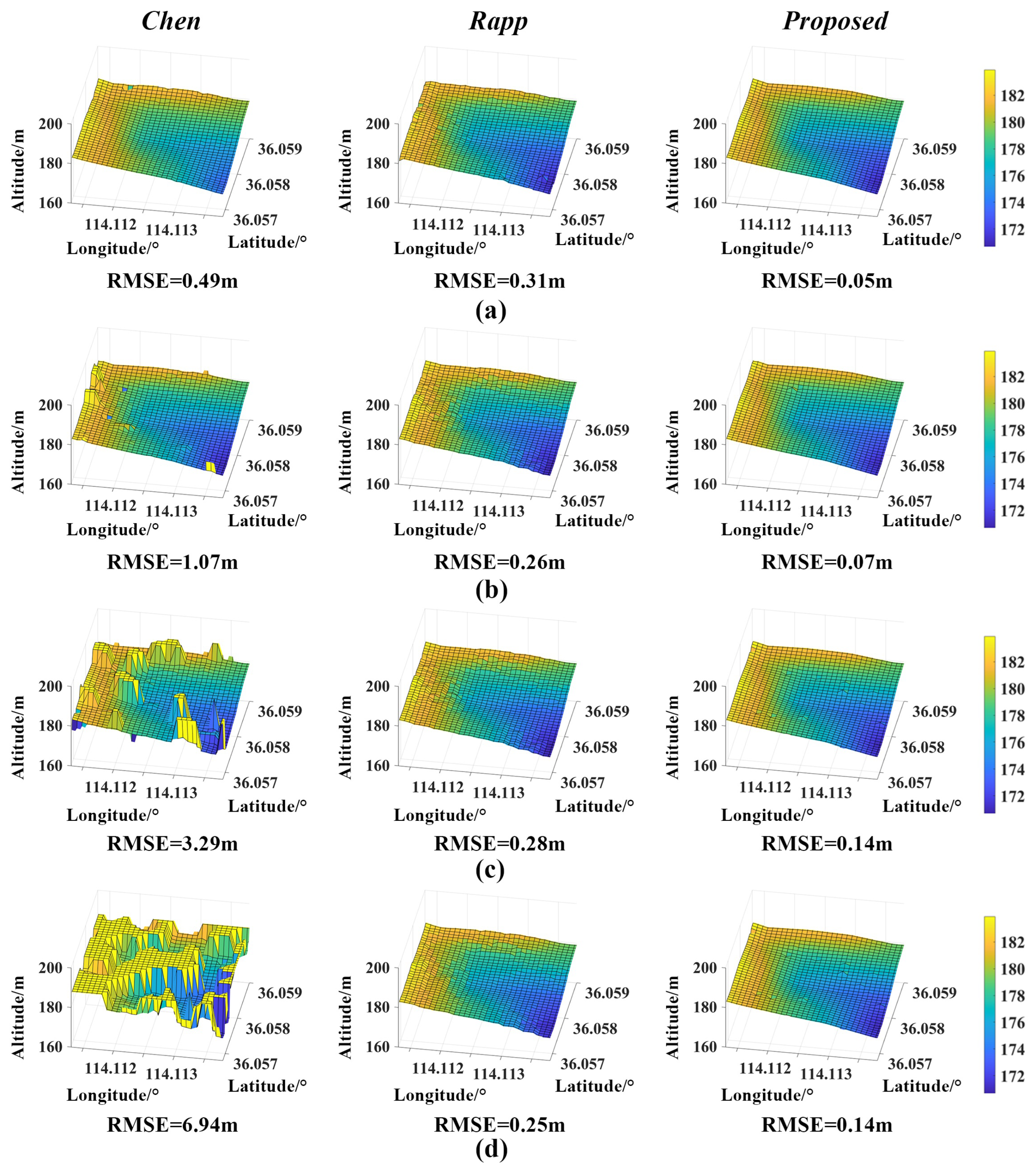
Figure 12.
Reconstruction results of undulating terrain 1. (a) Noise count rate @ 0.10 Mcps. (b) Noise count rate @ 0.77 Mcps. (c) Noise count rate @ 1.41 Mcps. (d) Noise count rate @ 1.84 Mcps.
Figure 12.
Reconstruction results of undulating terrain 1. (a) Noise count rate @ 0.10 Mcps. (b) Noise count rate @ 0.77 Mcps. (c) Noise count rate @ 1.41 Mcps. (d) Noise count rate @ 1.84 Mcps.
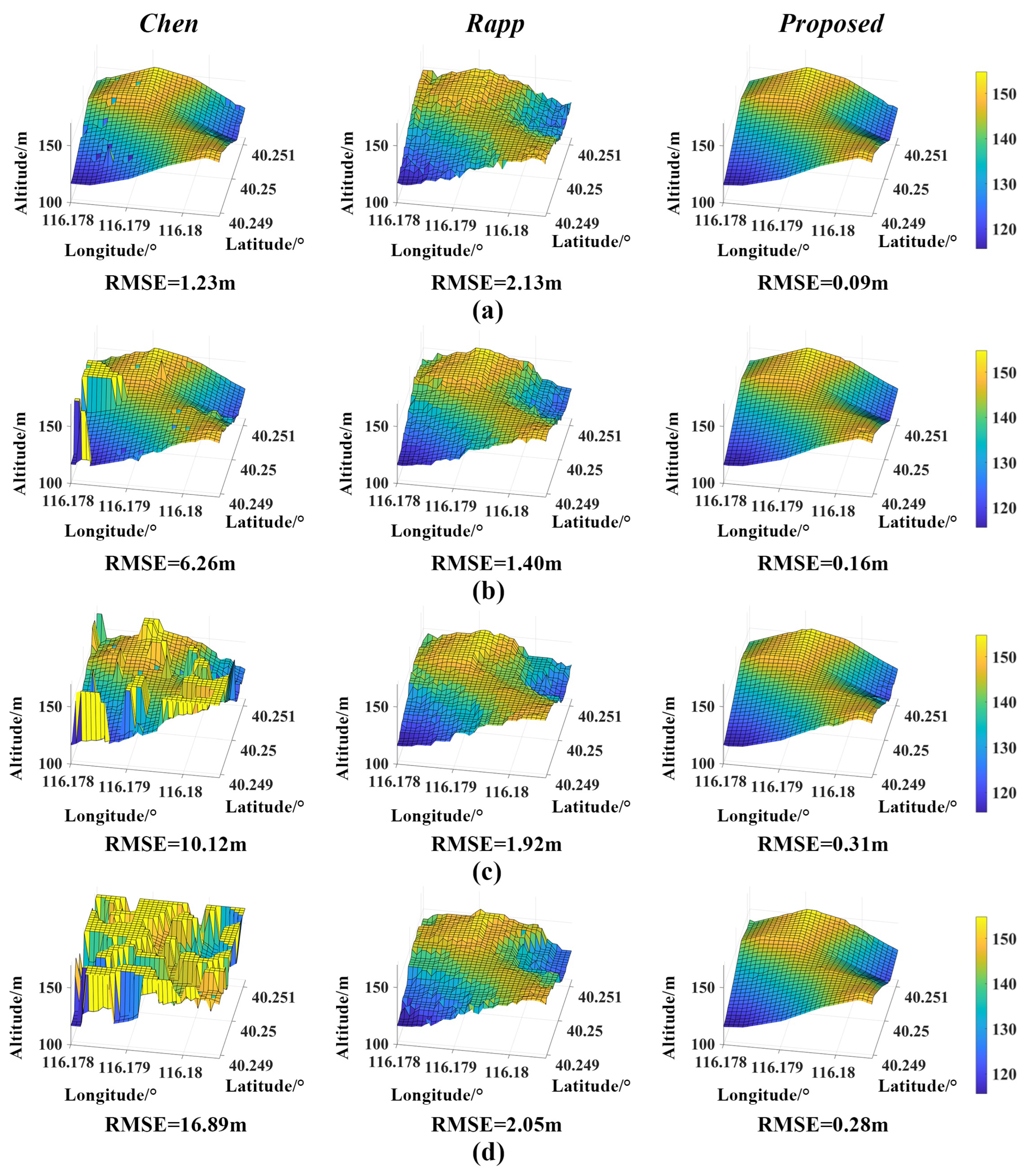
Figure 13.
Reconstruction results of undulating terrain 2. (a) Noise count rate @ 0.10 Mcps. (b) Noise count rate @ 0.77 Mcps. (c) Noise count rate @ 1.41 Mcps. (d) Noise count rate @ 1.84 Mcps.
Figure 13.
Reconstruction results of undulating terrain 2. (a) Noise count rate @ 0.10 Mcps. (b) Noise count rate @ 0.77 Mcps. (c) Noise count rate @ 1.41 Mcps. (d) Noise count rate @ 1.84 Mcps.
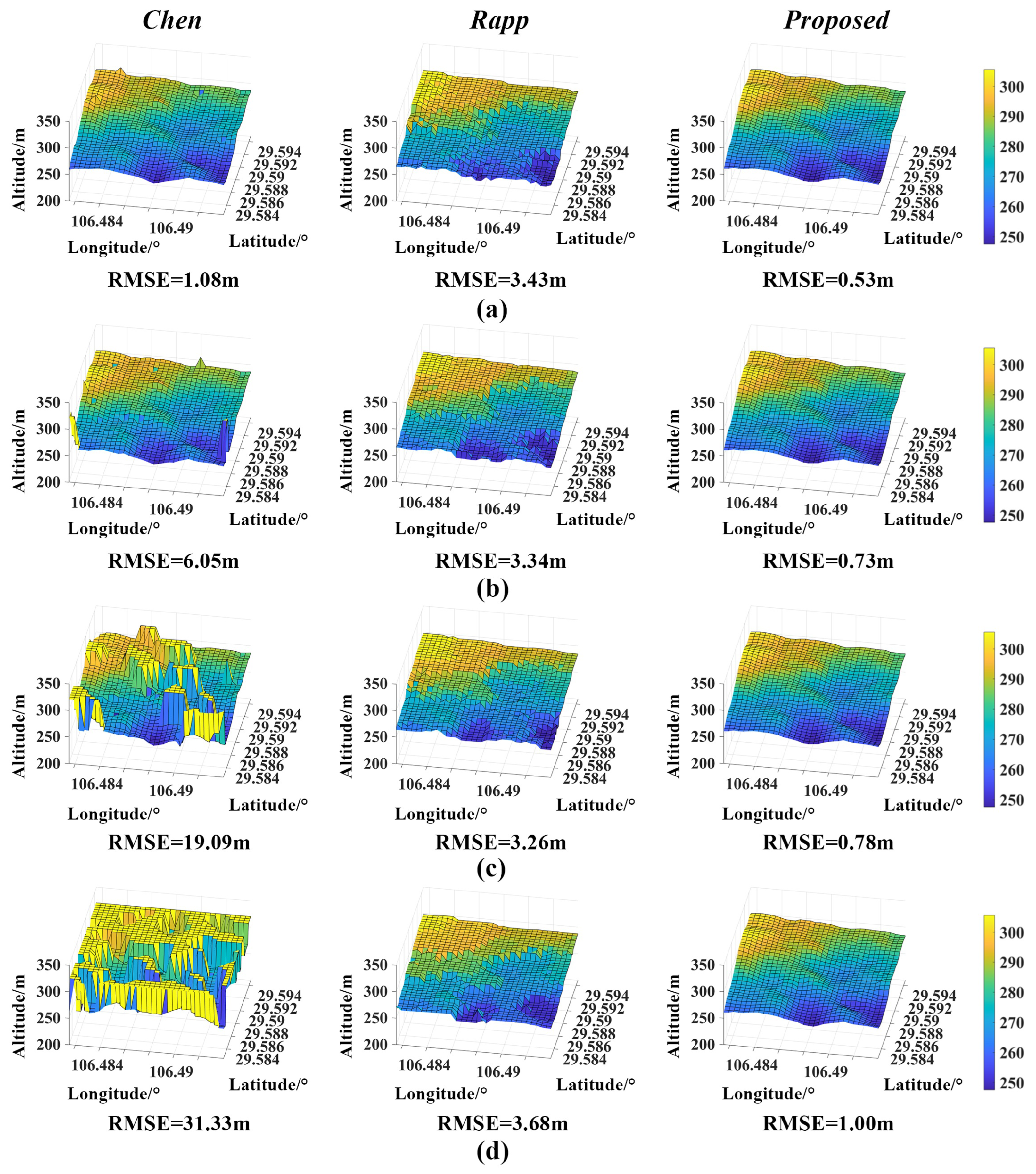
Figure 14.
Reconstruction results of undulating terrain 3. (a) Noise count rate @ 0.10 Mcps. (b) Noise count rate @ 0.77 Mcps. (c) Noise count rate @ 1.41 Mcps. (d) Noise count rate @ 1.84 Mcps.
Figure 14.
Reconstruction results of undulating terrain 3. (a) Noise count rate @ 0.10 Mcps. (b) Noise count rate @ 0.77 Mcps. (c) Noise count rate @ 1.41 Mcps. (d) Noise count rate @ 1.84 Mcps.
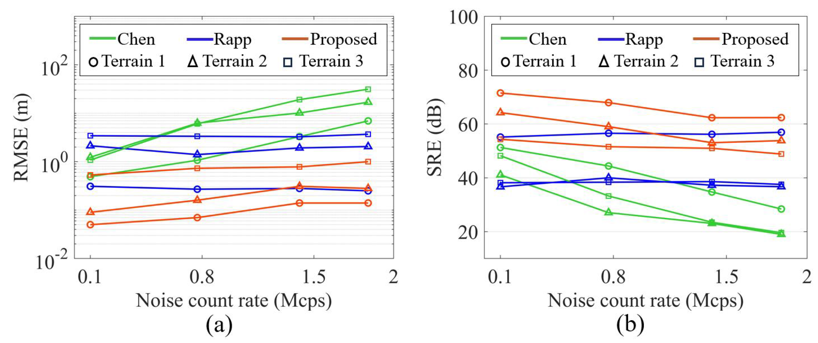
Figure 15.
The simulation results of three undulating terrains using different algorithms under different noise levels. (a) RMSE. (b) SRE.
Figure 15.
The simulation results of three undulating terrains using different algorithms under different noise levels. (a) RMSE. (b) SRE.
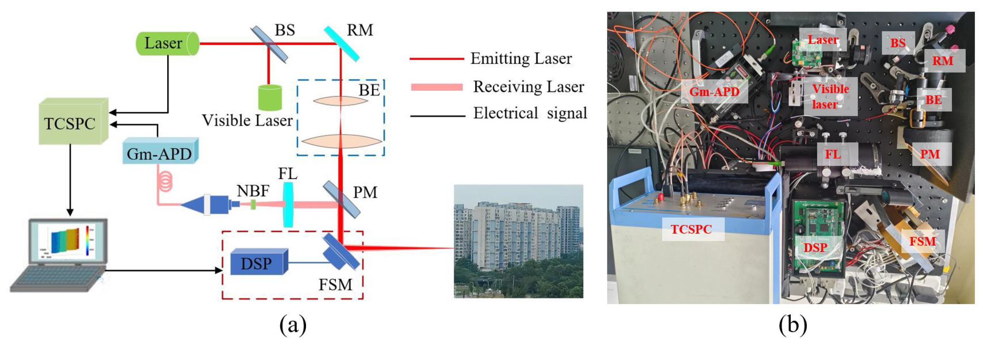
Figure 16.
Experimental setup of our photon counting LiDAR system. (a) Block diagram. (b) Physical image of the experimental device. BS, beam splitter; RM, reflecting mirror; BE, beam expander; PM, 45° perforated reflector; FL, optical focusing lens; NBF, narrow band-pass filter; FSM, fast steering mirror; DSP, digital signal processing; Gm-APD, Geiger mode avalanche photodiode.
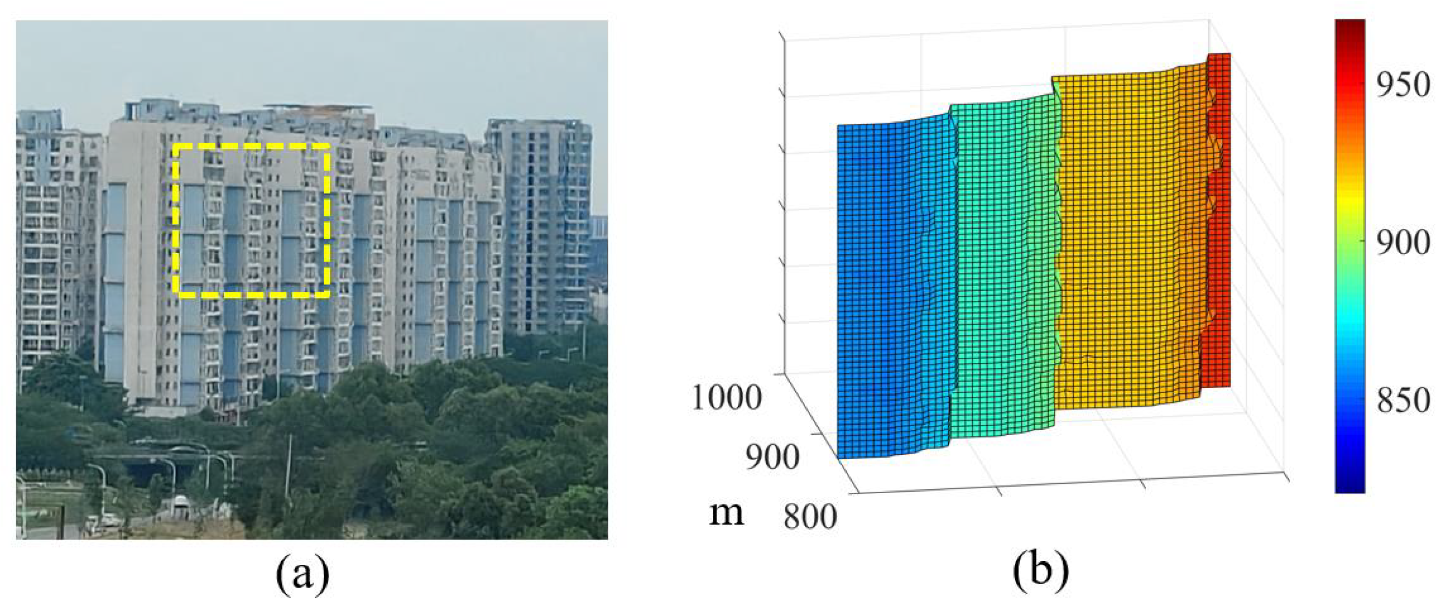
Figure 17.
(a) Image of the building in the visible light band in the range of 850–950 m. (b) Three-dimensional profile corresponding to the selected area shown in (a) (The yellow dashed frame indicates the range of the detection area).
Figure 17.
(a) Image of the building in the visible light band in the range of 850–950 m. (b) Three-dimensional profile corresponding to the selected area shown in (a) (The yellow dashed frame indicates the range of the detection area).
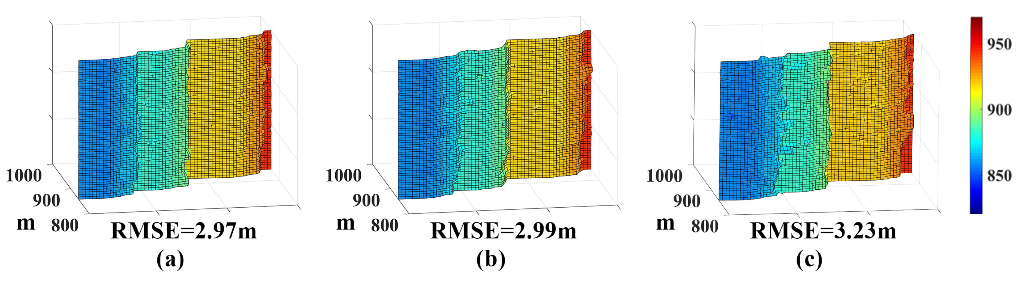
Figure 18.
The building depth estimation results obtained using the proposed method. (a) Noise count rate @ 0.23 Mcps. (b) Noise count rate @ 0.56 Mcps. (c) Noise count rate @ 1.02 Mcps.
Figure 18.
The building depth estimation results obtained using the proposed method. (a) Noise count rate @ 0.23 Mcps. (b) Noise count rate @ 0.56 Mcps. (c) Noise count rate @ 1.02 Mcps.
Table 1.
Application classification of the Bayesian algorithm in different sensors.
Table 1.
Application classification of the Bayesian algorithm in different sensors.
| Paper | Sensor | Approach |
|---|
| Gan [17] | SAR | Sparse Bayesian framework |
| Qu [18] | CCD | Dynamic Bayesian network |
| Riutort-Mayol [19] | CMOS | Bayesian multilevel random effects |
| Harpsoe [20] | EMCCD | Full Bayesian inference |
| Halimi [21] | Multispectral LiDAR | Hierarchical Bayesian |
| Tachella [22] | Photon counting LiDAR | Based on an area interaction process, Strauss process and RJ-MCMC |
| Altmann [23] | Photon counting LiDAR | Adaptive Markov chain and Monte Carlo method |
| Yang [24] | SAR and CCD sensor fusion | Variational Bayesian inference |
| Ravindran [25] | Camera, LiDAR and radar sensor fusion | CLR-BNN |
Table 2.
The RMSE and SRE results of different methods on terrain 1 with a depth variation of 13.3 m.
Table 2.
The RMSE and SRE results of different methods on terrain 1 with a depth variation of 13.3 m.
| Noise Count Rate (Mcps) | Method | RMSE (m) | SRE (dB) |
|---|
| | Chen | 0.49 | 51.27 |
| 0.10 | Rapp | 0.31 | 55.14 |
| | Proposed | 0.05 | 71.52 |
| | Chen | 1.07 | 44.39 |
| 0.77 | Rapp | 0.26 | 56.56 |
| | Proposed | 0.07 | 67.95 |
| | Chen | 3.29 | 34.72 |
| 1.41 | Rapp | 0.28 | 56.17 |
| | Proposed | 0.14 | 62.33 |
| | Chen | 6.94 | 28.41 |
| 1.84 | Rapp | 0.25 | 56.93 |
| | Proposed | 0.14 | 62.38 |
Table 3.
The RMSE and SRE results of different methods on terrain 2 with a depth variation of 39.2 m.
Table 3.
The RMSE and SRE results of different methods on terrain 2 with a depth variation of 39.2 m.
| Noise Count Rate (Mcps) | Method | RMSE (m) | SRE (dB) |
|---|
| | Chen | 1.23 | 41.09 |
| 0.10 | Rapp | 2.13 | 36.35 |
| | Proposed | 0.09 | 64.23 |
| | Chen | 6.26 | 27.05 |
| 0.77 | Rapp | 1.40 | 40.00 |
| | Proposed | 0.16 | 59.01 |
| | Chen | 10.12 | 23.05 |
| 1.41 | Rapp | 1.92 | 37.24 |
| | Proposed | 0.31 | 53.05 |
| | Chen | 16.89 | 18.98 |
| 1.84 | Rapp | 2.05 | 36.70 |
| | Proposed | 0.28 | 53.82 |
Table 4.
The RMSE and SRE results of different methods on terrain 3 with a depth variation of 58.1 m.
Table 4.
The RMSE and SRE results of different methods on terrain 3 with a depth variation of 58.1 m.
| Noise Count Rate (Mcps) | Method | RMSE (m) | SRE (dB) |
|---|
| | Chen | 1.08 | 48.22 |
| 0.10 | Rapp | 3.43 | 38.16 |
| | Proposed | 0.53 | 54.32 |
| | Chen | 6.05 | 33.24 |
| 0.77 | Rapp | 3.34 | 38.37 |
| | Proposed | 0.73 | 51.56 |
| | Chen | 19.09 | 23.48 |
| 1.41 | Rapp | 3.26 | 38.59 |
| | Proposed | 0.78 | 50.97 |
| | Chen | 31.33 | 19.60 |
| 1.84 | Rapp | 3.68 | 37.54 |
| | Proposed | 1.00 | 48.84 |
Table 5.
Main parameters of the experimental system.
Table 5.
Main parameters of the experimental system.
| Parameter | Value |
|---|
| Wavelength | 1064 nm |
| Pulse width | 3.5 ns |
| Time resolution | 64 ps |
| Laser divergence angle | 1.13 mrad |
| Dead time | 41.3 ns |
| Filter bandwidth | ±3 nm |
| Photon detection efficiency | 2.8% |
| Pulse repetition frequency | 5–6 kHz |
Table 6.
The RMSE and SRE results of different methods on an outdoor building at a distance of 850–950 m.
Table 6.
The RMSE and SRE results of different methods on an outdoor building at a distance of 850–950 m.
| Noise Count Rate (Mcps) | SBR | Method | RMSE (m) | SRE (dB) |
|---|
| | | Chen | 3.73 | 47.61 |
| 0.23 | 0.17 | Rapp | 3.73 | 47.61 |
| | | Proposed | 2.97 | 49.60 |
| | | Chen | 4.11 | 46.75 |
| 0.56 | 0.06 | Rapp | 3.31 | 48.64 |
| | | Proposed | 2.99 | 49.52 |
| | | Chen | 6.18 | 43.20 |
| 1.02 | 0.03 | Rapp | 3.78 | 47.51 |
| | | Proposed | 3.23 | 48.86 |


 ,
, 


