HCM-LMB Filter: Pedestrian Number Estimation with Millimeter-Wave Radar in Closed Spaces

Abstract

The electromagnetic wave transmitted by the millimeter-wave radar can penetrate flames, smoke, and the high-temperature field, and is the main sensor for detecting disaster victims in closed spaces. However, a moving target in the closed space will produce a considerable number of false detections in the point cloud data collected by the radar due to multipath scattering. The false detections lead to false trajectories generated by multi-target tracking filters, such as the labeled multi-Bernoulli (LMB) filter, which, therefore, leads to inaccurate estimation of the number of pedestrians. Addressing this problem, in this paper, a three-class combination of the clutter point clouds model is proposed: static clutter, non-continuous dynamic clutter (NCDC), and continuous dynamic clutter (CDC). The model is based on the spatial and temporal distribution characteristics of the CDC sequence captured by a two-dimensional (2D) millimeter-wave (MMW) radar. However, in open space, CDC appears infrequently in radar tracking applications, and thus has not been considered in multi-target tracking filters such as the LMB filter. This leads to confusion between the CDC point cloud collected by the high-resolution radar in closed spaces and the real-target point cloud. To solve this problem, the impact mechanism of the LMB filter on prediction, update, and state estimation is modeled in this paper in different stages based on the temporal and spatial distribution characteristics of CDC. Finally, a hybrid clutter model-based LMB filter (HCM-LMB) is proposed, which focuses on scenes where NCDC and CDC are mixed. The filter introduces the temporal and spatial distribution characteristics of NCDC based on the original LMB filter, and improves the prediction, update, and state estimation of the original filter by combining the impact mechanism model and the new CDC prediction, CDC estimation, and false trajectory label management algorithm. Experiments were conducted on pedestrians in building corridors using 2D MMW radar perception. The experimental results show that under the influence of CDC, the total number of pedestrians estimated by the HCM-LMB filter was reduced by 22.5% compared with that estimated by the LMB filter.

1. Introduction

In closed spaces such as large building complexes or underground roads, emergencies such as fires can quickly produce a large amount of smoke. This makes the detection performance of sensors such as cameras and lidars sharply drop, making it difficult to indicate reliable pedestrian number information for disaster relief operations. The electromagnetic wave transmitted by the millimeter-wave radar can penetrate smoke, flames, and high-temperature fields [1,2,3], and this is one of the main sensors used for target detection and pedestrian number estimation in disaster situations. Therefore, it is of great significance to study the estimation method of the pedestrian target number based on the MMW radar in closed spaces.

Due to the strong adaptability of the 2D MMW radar in open environments, the existing research primarily employs two techniques to estimate the target number: clustering and estimation of the extended information of targets [1]. However, in closed spaces, the radar will be subjected to higher-intensity multipath scattering, leading to a significant number of false detections and uncertainty of data, when the radar is detecting high-resolution point cloud data for moving targets in close-range. Therefore, the impact mechanism of multipath point cloud data on existing clustering or multiple-target tracking techniques, as well as the processing methods for false detection point clouds for these two techniques, will have a direct and significant effect on estimating the number of pedestrians in closed spaces.

A common view is that time series anomaly detection methods can be used to identify and remove false detection point clouds. This is equivalent to representing false detection point clouds as outliers relative to some standard or common signal. Common anomaly detection methods include methods based on statistical models, methods based on deep learning models, and methods based on machine learning models [4]. Methods based on deep learning models rely on a large amount of labeled data for supervised training and have the characteristics of high accuracy and strong generalization, but there is a lack of large-scale datasets in the field of radar false-alarm point cloud detection. Machine learning models also require training of the model, but on the one hand, they have lower requirements for the sample size, and on the other hand, they can use unsupervised learning techniques such as clustering, which do not require labeling of the samples. The advantage of statistical model methods is that they have low complexity, a fast computation speed, and a strong generalization ability. Since there is no training process, they can be quickly put into production even without prior data accumulation. The following will further analyze the statistical and machine learning models based on clustering techniques.

Density-based clustering algorithms, such as density-based spatial clustering of applications with noise (DBSCAN) [5], mean-shift [6], and others [7,8,9], are able to automatically identify the optimal number of clusters and outliers. The idea of these algorithms is to assume that the datasets of different clusters conform to different probability density distributions, which can be estimated by the Mahalanobis distance. Sample points will converge at the maximum local density. However, the biggest drawback is that it is necessary to set parameters such as the radius or bandwidth instead of the number of targets. These parameters or features are not directly related to the number of targets, and the number of targets is susceptible to outliers caused by clutter. Therefore, whether the density difference between the two types of point clouds is substantial enough decides whether the density-based clustering algorithm can separate the false-target point cloud from the real-target-detection point cloud. When the density difference is small, it is difficult to distinguish by density alone, resulting in false-target problems.

Statistical model-based anomaly detection methods mainly include methods based on statistical criteria, test-based methods, and filter methods [10]. The first two methods rely on the residual error between the true value and the predicted value. This means that the prior distribution of the ideal data needs to be known, and then the statistics of the prior distribution, such as the mean variance or specific probability density function, are used for hard threshold filtering or hypothesis testing to remove outliers [11,12]. For the pedestrian number estimation problem based on the radar point cloud, which is the focus of this paper, the temporal and spatial distribution of the normal pedestrian point cloud does not conform to any standard distribution. In comparison, the filter-based method adopts an online learning architecture, which can learn the temporal and spatial characteristics’ distribution of the point cloud in real time according to the prior assumption and the change of actual observation data. In addition, the filter-based method can integrate multiple target ID management methods and solve the anomaly detection and multi-target number estimation problem in a one-stage target state estimation framework. It is different from the statistical criteria or test-based methods, which need to eliminate outliers and then tracking by using filters (two-stage).

The target state estimated by the multi-target tracking filters contains the target identity information, usually the ID or the label, which can be used to estimate the target number. The first widely used multi-target tracking technology combined data association and the Kalman filter, including global nearest neighbor (GNN) [13] and joint probabilistic data association (JPDA) [14]. After that, aiming at the combination explosion problem when there are many targets and measurements, multiple hypothesis tracking (MHT) and other methods combining the advantages of GNN and JPDA algorithms were proposed [15], but there were problems of inaccurate target number estimation due to the decline of the data association effect in high-density targets or high-noise environments.

The probability hypothesis density (PHD) filter [16,17,18,19] replaced the data association method for multi-target tracking via the use of random finite set (RFS) theory. This technique can turn the multi-target state estimation problem into a posterior probability hypothesis density solution problem, which is advantageous in lowering the computation complexity. This yields a conducive environment and a unified theoretical framework for integrating more elements that cause dynamic changes in the target number into multi-target state estimation. However, the PHD filter uses a first-order moment to approximate the posterior probability density, which makes it difficult to ensure that each target has a unique and continuous ID and will lead to unstable results of time-varying target number estimation.

To improve the performance of target number estimation, the cardinalized probability hypothesis density (CPHD) [20,21] was proposed by Mahler, which jointly propagates the first-order and second-order moments in Bayesian recursion. At the same time, the multi-target multi-Bernoulli (MeMBer) [18] filter proposed by Mahler and the cardinalized balanced multi-target multi-Bernoulli (CBMeMBer) [22] filter proposed by Vo et al. propagate parameters of the multi-Bernoulli RFS that approximate the posterior probability density and focus on tracking targets that can appear or disappear from the field-of-view [23]. Since then, in order to obtain better performance, Vo et al. proposed a class of multi-target tracking filters based on the labeled RFS theory and the multi-Bernoulli filter that can generate trajectories while estimating targets’ states and are closed under the Chapman–Kolmogorov equation. Those filters are represented by the delta generalized labeled multi-Bernoulli (δ-GLMB) [24,25,26,27] filter and the labeled multi-Bernoulli (LMB) [28,29] filter. As an efficient approximation of the δ-GLMB, the LMB filter’s tracking accuracy is very close to that of the δ-GLMB filter. Therefore, the LMB filter can be used as a baseline model for the improved target number estimation method in this paper.

In open space, the impact of clutter on target number estimation can be moderately controlled by the target number estimation algorithm using filters such as the LMB filter and others at a relatively low level. However, the clutter model that follows Poisson distribution used in these filters is based on the spatial–temporal distribution characteristics of the open-space clutter model. It is quite different from the clutter characteristics in closed spaces, which is primarily because millimeter-wave radar is susceptible to stronger multipath effects in closed spaces. The spatial–temporal distribution characteristics of point clouds affected by the multipath effect, especially the point cloud density, are similar to those of a real target, unlike the uninterested point clouds observed in open spaces.

RFS-based tracking algorithms are progressively being used in other areas, such as traffic monitoring. While most of the scenarios in these applications are in open spaces, the applications in closed spaces face more challenges. For example, the authors of [30] separate interferences such as pedestrians from vehicles by the signal-to-noise ratio (SNR), but our application scenario contains only pedestrians, which are difficult to separate from each other by SNR. The authors of [31] track the target by estimating its shape and other features of the point cloud while tracking, but our data contain pedestrians collected in closed spaces with a restricted field-of-view, and the data are affected by occlusion and multipath interference, etc., so some point cloud data of the target do not have the characteristics of an extended target, but appear as a point target or are missed. The authors of [32,33] improved the tracking accuracy by adding road restrictions and interactions between vehicles, but did not consider the interference caused by multipath effects. The object of our study is pedestrians, whose trajectory is relatively unpredictable, and the site information has limited improvement on the target number estimation and tracking effect.

Aiming at the problem that false tracking data exist in the LMB filter, in this paper, a spatial–temporal distribution feature model of two-dimensional point cloud data of moving pedestrians in closed-space scenarios using the millimeter-wave radar is analyzed and constructed. This hybrid clutter model (HCM) in closed space divides the data noise into three categories: static clutter, non-continuous dynamic clutter, and continuous dynamic clutter caused by radar indoor multipath scattering. Among them, the dynamic multipath noise sequence has a high similarity with the moving target sequence, which is the main reason for the decrease of the multi-target tracking accuracy and the target number estimation bias. The spatial–temporal feature model of dynamic multipath noise is used in this paper to highlight the feature differences between dynamic multipath noise and the real-target trajectory. In addition, the impact of dynamic multipath noise on the prediction, update, and state estimation stages of the LMB filter in the closed-space scenario is analyzed, along with the reasons for the final target number estimation bias. To reduce the influence of dynamic multipath noise in the update stage, an intensity function of dynamic multipath noise is developed and applied to the LMB filter. Finally, to address the problem of target number estimation bias caused by dynamic multipath noise on the LMB filter, a hybrid clutter model-based LMB (HCM-LMB) filter is proposed. This filter introduces the dynamic multipath noise feature model, improves the original noise model of the LMB filter, and builds a false-trajectory label management mechanism.

This paper is organized as follows: the hybrid clutter model in a closed space is introduced in the Section 2, and the Section 3 analyzes the influence of continuous dynamic clutter on the LMB filter. Section 4 introduces the HCM-LMB filter, while Section 5 includes the introduction of experimental data acquisition, verification experiments, and comparative experiments. Finally, we summarize our algorithm and experiment results in Section 6.

2. Clutter Model in Closed Space

By examining the characteristics of the spatial distribution and spatial–temporal distribution of the point cloud data collected by the 2D MMW radar in a closed space, the uninterested points of the data were divided into three categories: static clutter, non-continuous dynamic clutter, and continuous dynamic clutter, as follows:

• Static clutter—points with zero velocity in the point cloud data—is generated by the environment or static targets. The Doppler frequency shift of stationary targets is close to zero, while the Doppler frequency shift of moving targets is related to the relative motion speed of the target and the radar, which is generally non-zero. Therefore, in the process of radar point cloud generation, since the relative motion speed between the radar and the wall cladding is zero, the multipath scattering of the wall has a Doppler frequency shift close to zero, which will be directly filtered out by the radar processor, and there is a low probability of generating such multipath point clouds. However, there is relative motion between the pedestrian and the radar, and both direct scattering point clouds and multipath point clouds will be retained by the radar processor.
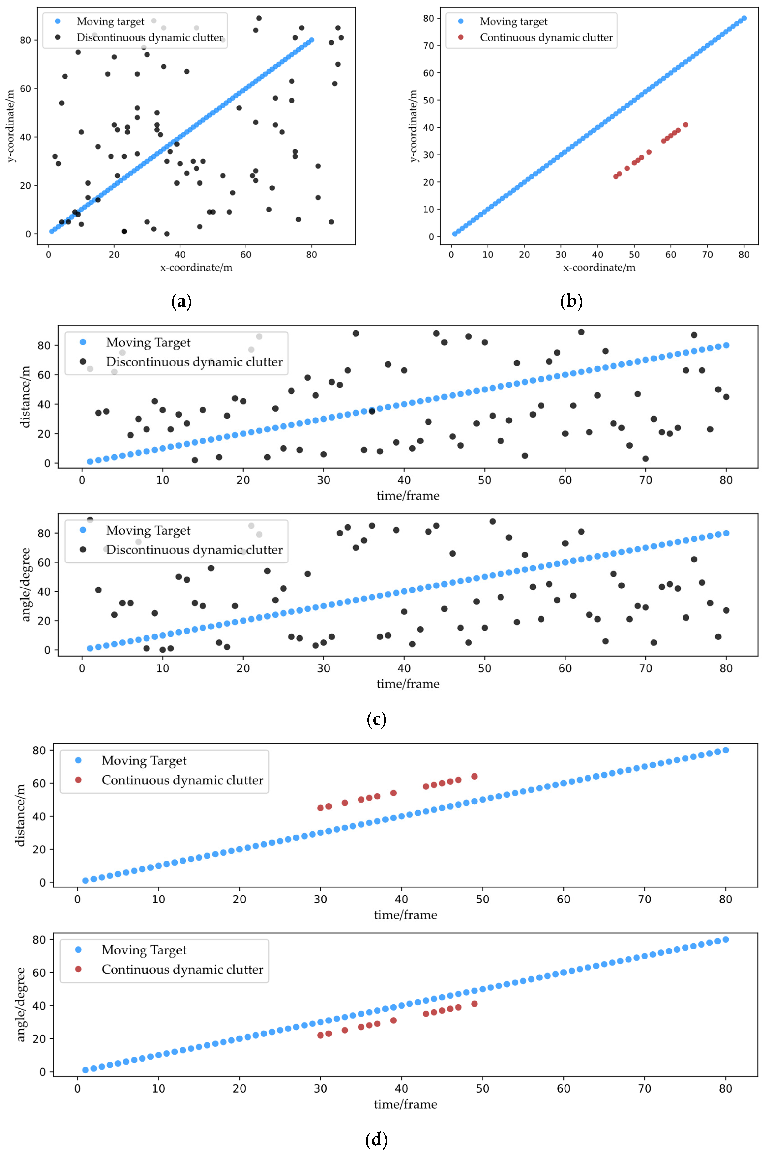
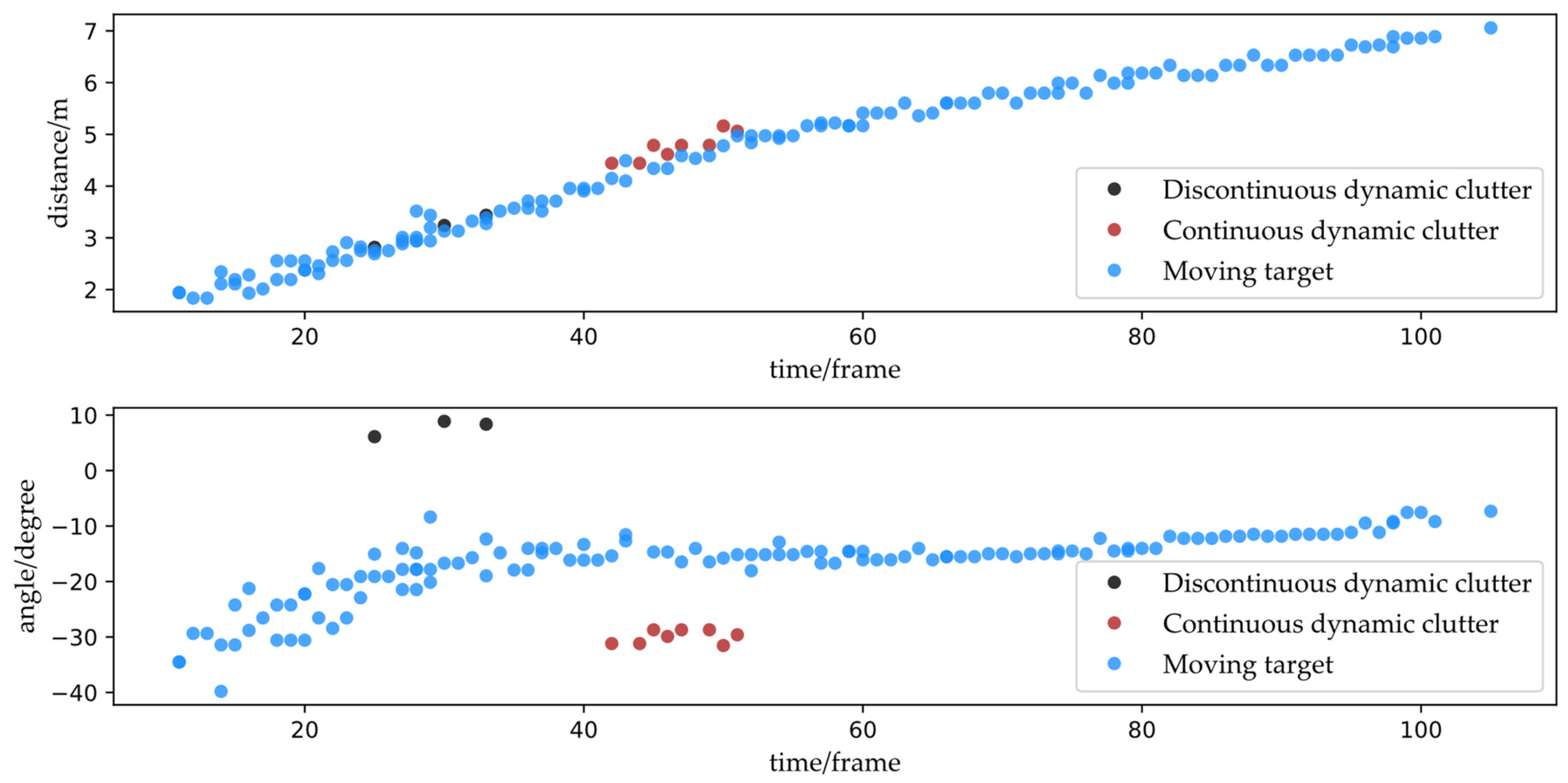
• Non-continuous dynamic clutter (abbreviated as “NCDC” in the following), with non-zero velocity, is generally multipath clutter generated by moving targets or noise generated by random environments. When comparing the spatial distribution of NCDC and moving target observations, NCDC is often distributed more scatteringly and can be regarded as independent of other NCDC or the moving targets. Its sequence also clearly shows discontinuity, making it more challenging to create a continuous sequence characteristic. Figure 1a,b, respectively, depict the simulation diagrams of the spatial and the spatial–temporal distributions of NCDC and moving target observations.
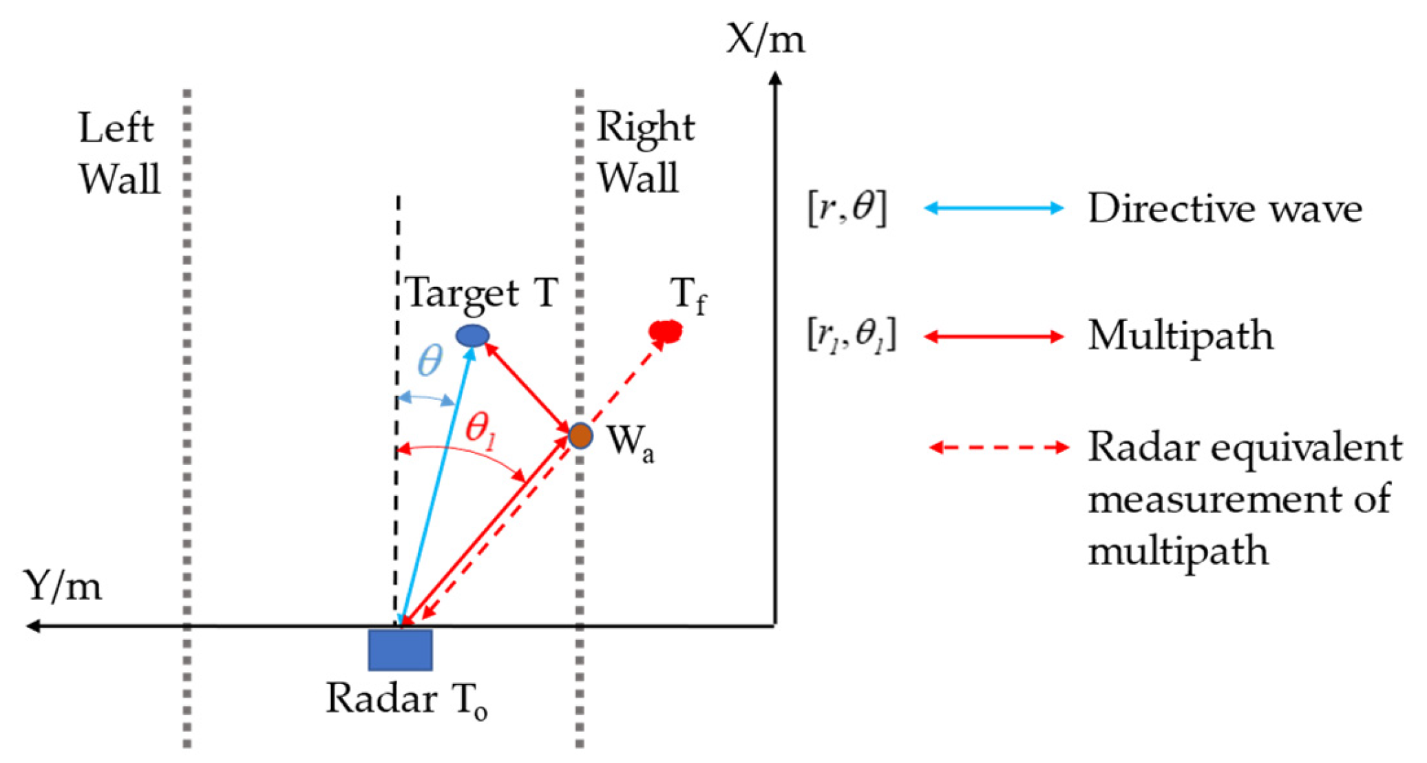
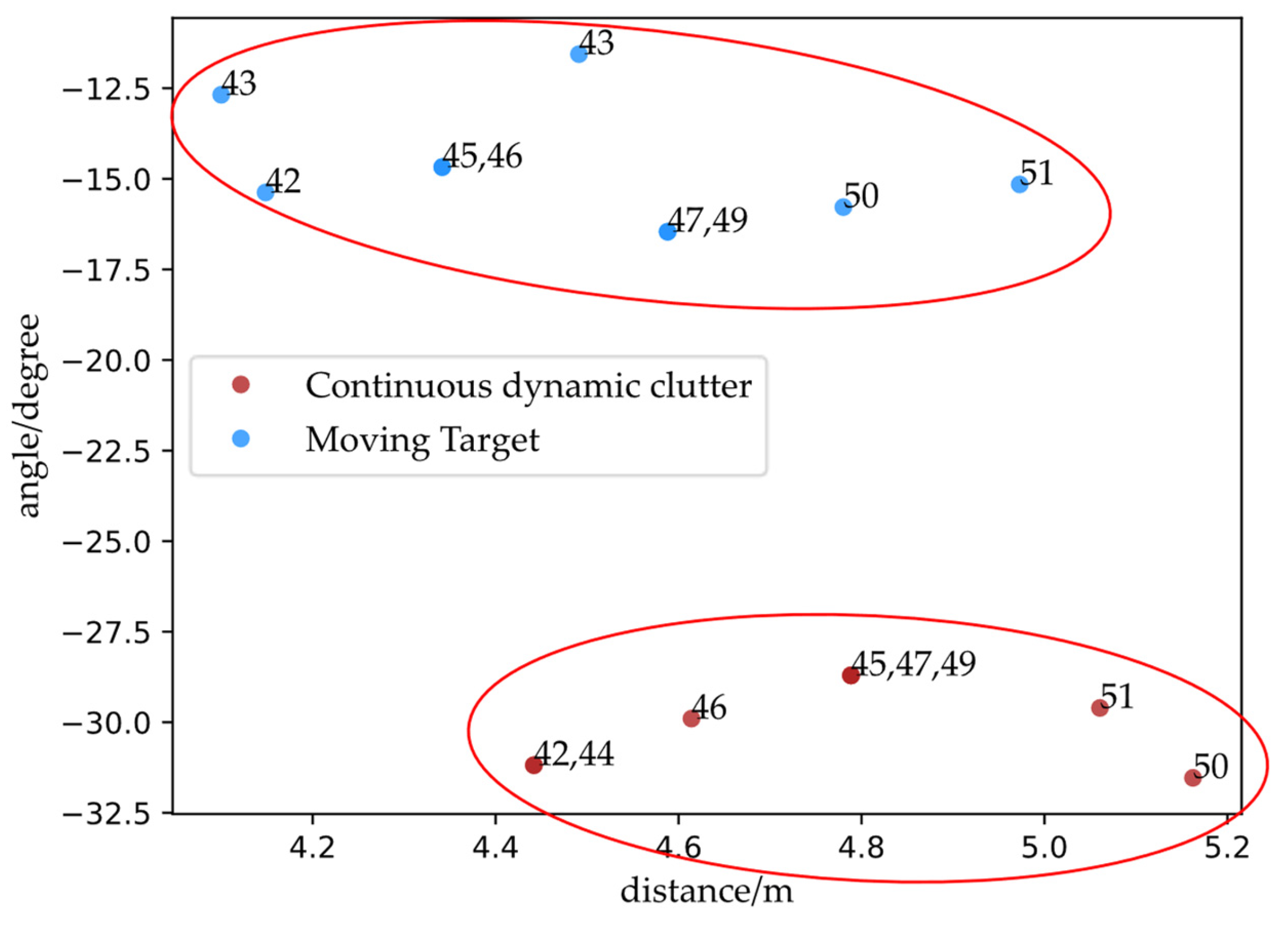
• Continuous dynamic clutter, caused by radar indoor multipath scattering (abbreviated as “CDC” in the following) with non-zero velocity, are points generated from a moving target by multipath wave. A moving target usually generates at most one CDC point in a frame, which may be because the power of the multipath wave is significantly lower than that of the direct wave power, so it is difficult to observe higher-order multipath scattering detected through the constant false-alarm rate (CFAR) detection of the radar. Although the CDC sequence shows a shorter duration and is sparser than the moving target sequence, it nevertheless displays continuity and similarity to the trajectory detected by the direct wave from the same moving target. Figure 1c,d show the simulation diagrams of the spatial–temporal distribution of the CDC and the moving target observations, respectively.

The spatial similarity between the CDC sequence and its related moving target sequences detected by the direct wave can be directly perceived from the above figure, and both sequences exhibited some continuity. This is an important reason why CDC sequences are prone to be estimated as “false targets”. Therefore, finding the characteristics to distinguish the two is a focus of this study.

In order to find the characteristics that make the CDC sequence distinctive from the direct wave observation sequence of the moving target, it is necessary to analyze the CDC sequence in terms of its primary cause, the multipath effect. Figure 2 is a schematic diagram of the multipath effect wherein a MMV radar is detecting a moving target, where the solid blue line is the direct wave from the radar to the moving target, $T$, the solid red line is the multipath from the radar coordinate system, $T_0$, passing through the reflection point of the wall, $W_a$, reaching the moving target, $T$, and then returning to the radar. The detection through the solid red line is equivalent to the dashed red line, and then generates the measurement points, $T_f$.

The coordinates $\left[r,\mathsf{\theta }\right]$ and $\left[r_1,{\mathsf{\theta }}_1\right]$ of the moving target $T$ and the dynamic equivalence point $T_f$ of the multipath with respect to the radar origin $T_0$ satisfy:

$$r=r_{T_{0}T}$$

(1)

$$\mathsf{\theta }={\mathsf{\theta }}_{T_{0}T}$$

(2)

$$r_1=\frac{r_{T_0{W}_a}+r_{W_{a}T}+r_{T{T}_0}}{2}$$

(3)

$${\mathsf{\theta }}_1={\mathsf{\theta }}_{T_0{W}_a}$$

(4)

From Figure 2 and Equations (1) and (3), we know $r_{T_{0}Wa}+r_{WaT}>r_{T_{0}T}$, so it can be observed that the CDC’s distance is larger than that of its related moving target point, i.e., $r_1>r$. In the scene of Figure 2, if the moving target moves continuously and linearly, and the multipath generates a continuous equivalent observation sequence over a period of time, the angle ${\mathsf{\theta }}_1$ will also change in a certain range with the moving direction of the moving target.

The CDC sequence affected by the multipath effect is related to the reflection point $W_a$; however, in the application scenario, the reflection point may not necessarily be a wall, it could also be other pedestrians. Due to the random motion of the observed moving target pedestrians and the low angular resolution of the 2D millimeter-wave radar, the wall position is of limited use as a priori information to remove false trajectories.

Consequently, if the moving target moves continuously, the CDC sequence caused by radar indoor multipath scattering has the following characteristics:

• CDC’s distance is related to the geometry of the moving target and the reflection point, and the value is greater than the direct wave observation related to it.
• The angle is related to the location of the moving target.
• A moving target does not generate or generates only one CDC passing through the same reflector at the same moment.

The statistical validation of the above characteristics using data collected in the closed space is described in Section 5.2, where the detection rates of the two dynamic clutter sequences and their related moving target sequences are used to verify the continuity of the sequences, and the Pearson correlation coefficients between the sequence features are used to verify the correlation of the sequences, which is:

$${\rho }_{XY}=\frac{{\displaystyle \sum \left(X-\overline{X}\right)\left(Y-\overline{Y}\right)}}{\left(\sqrt{{\displaystyle \sum _{i=1}^n{\left(X_i-\overline{X}\right)}^2}}\right)\left(\sqrt{{\displaystyle \sum _{i=1}^n{\left(Y_i-\overline{Y}\right)}^2}}\right)}$$

(5)

where $X$ and $Y$ represent different sets of characteristics of the sequence, respectively.

3. Influence of Continuous Dynamic Clutter on LMB Filter

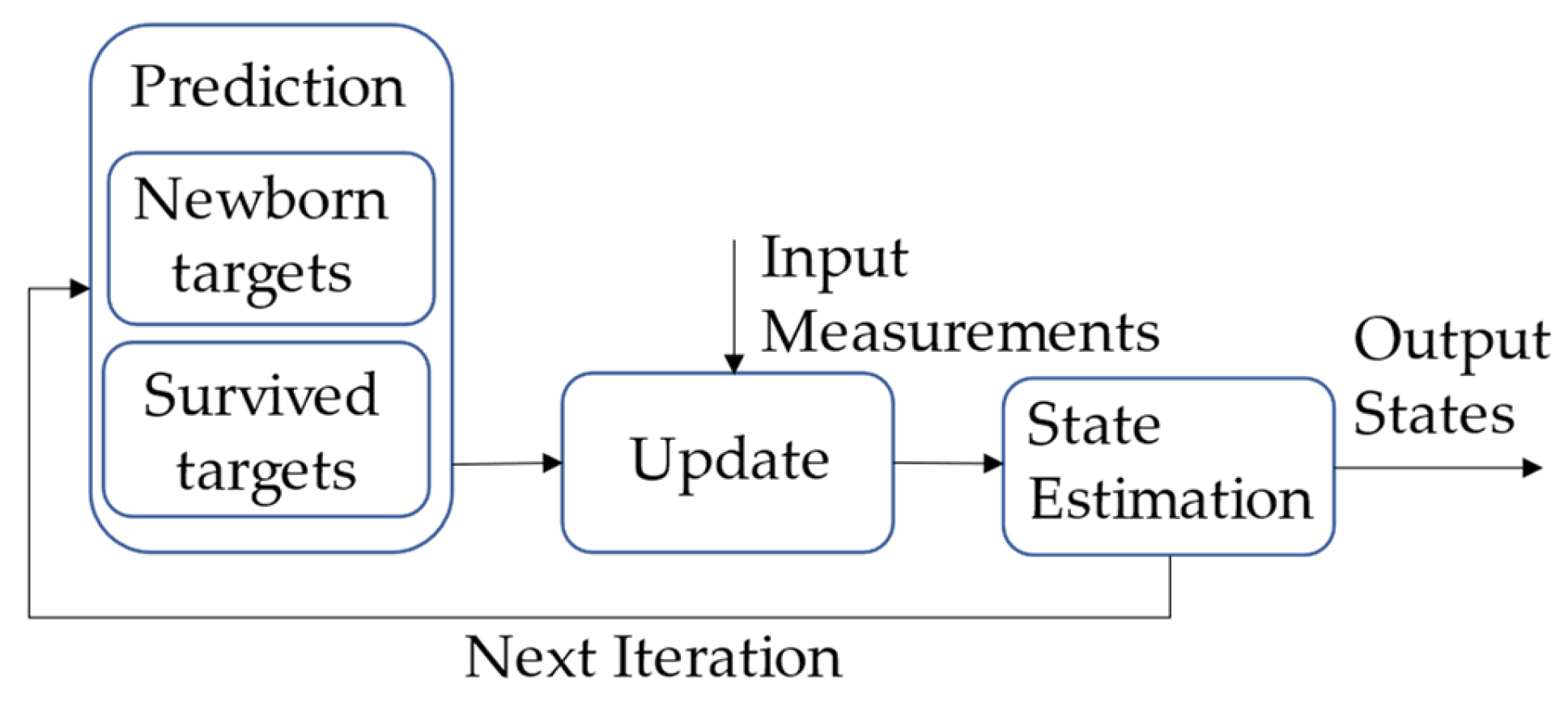
3.1. Introduction of Labeled Multi-Bernoulli Filter

It is known that the CDC sequence caused by radar indoor multipath scattering has a high similarity with the moving target trajectory and is the main cause of the false trajectory. It is crucial to analyze the reasons for the cardinality bias and false trajectories caused by CDCs, and therefore, distinguish the CDCs from the real-target trajectory.

The scheme of the LMB filter is shown in Figure 3, which includes three main stages: prediction, update, and state estimation. The LMB filter approximates the Bayes multi-target filter, which approximates predicted and posterior densities of a target as a labeled multi-Bernoulli process [29]. Therefore, the predicted and posterior densities are described as the densities of LMB RFSs.

In the prediction stage, the target states to be processed consist of two categories: the newborn target, generated by the birth model, and the survived target, estimated from the previous iteration. Symbols related to newborn targets are identified by the subscript “B” and symbols related to targets estimated from the previous iteration, also known as the “survived target” or “a priori”, are identified by the subscript “S” in the following part of this paper. Each target trajectory is identified by a unique label, $\mathcal{l}=(k,i)$, in discrete label space $\mathbb{L}$ to the state $x$ in state space $\mathbb{X}$, where $k$ is the birth time of the target and $i$ is a unique index.

Then, in the update stage, the newborn targets and survived targets are merged into a set of “predicted targets”, which will be identified by the subscript “+”. The updated targets’ states are calculated by predicted target states, along with the measurements.

Finally, in the state estimation stage, the updated targets are pruned according to the parameters of their posterior densities. The remaining target states are also prior states in the next iteration. Nevertheless, only some of the updated states are extracted as real-target states and output. Besides, the states’ extraction is based on the cardinality that is simultaneously calculated by the LMB filter.

In the following, the iteration at time k is omitted for convenience. We follow the notations representation of LMB filters in the literature [28].

A label, $\mathcal{l}\in \mathbb{L}$, is appended in the state $x\in \mathbb{X}$ as the identity of the trajectory. Define $\mathcal{L}\left(\left(x,\mathcal{l}\right)\right)=\mathcal{l}$ as the projection from the discrete label space $\mathbb{L}$ to state space $\mathbb{X}$. Then, $\mathcal{L}\left(x\right)=\left\{\mathcal{L}\left(x\right):x\in X\right\}$ gives a LMB RFS the set of labels, where $\mathcal{L}:\mathbb{X}\times \mathbb{L}\to \mathbb{L}$. To identify the targets, ensure the cardinality of the label set equals the cardinality of the state vectors set, i.e., $\left|\mathcal{L}\left(\mathbf{X}\right)\right|=\left|\mathbf{X}\right|$, by using the distinct label indicator:

$$\Delta \left(\mathbf{X}\right)={\delta }_{\left|\mathrm{X}\right|}\left(\mathcal{L}\left(\mathbf{X}\right)\right)$$

(6)

The LMB filter describes the predicted and posterior multi-target densities as LMB RFSs, with the parameter set $\pi ={\{r^{(\mathcal{l})},p{(x)}^{(\mathcal{l})}\}}_{\mathcal{l}\in \mathbb{L}}$, which can be simplified to:

$$\pi \left(\mathbf{X}\right)=\Delta \left(\mathbf{X}\right)w\left(\mathcal{L}\left(\mathbf{X}\right)\right)p^{\mathbf{X}}$$

(7)

$$w\left(L\right)={\displaystyle \prod _{i\in \mathbb{L}}\left(1-r^{\left(i\right)}\right)}{\displaystyle \prod _{\mathcal{l}\in L}\frac{l_{\mathbb{L}}\left(\mathcal{l}\right)r^{\left(\mathcal{l}\right)}}{1-r^{\left(\mathcal{l}\right)}}}$$

(8)

$$p\left(x,\mathcal{l}\right)=p^{\left(\mathcal{l}\right)}\left(x\right)$$

(9)

The parameter set $\pi$ contains the existence probability, $r^{\left(\mathcal{l}\right)}$, of the trajectory with the label $\mathcal{l}$ and the spatial distribution, $p\left(x\right)$, and $1-r^{\left(\mathcal{l}\right)}$ represents the missed detection rate of the trajectory.

The cardinality distribution of a LMB RFS is as follows:

$$\rho \left(n\right)={\displaystyle \prod _{i\in \mathbb{L}}\left(1-r^{\left(i\right)}\right)}\cdot {\displaystyle \sum _{L\in {\mathcal{F}}_n\left(\mathbb{L}\right)}{\displaystyle \prod _{\mathcal{l}\in L}\frac{r^{\left(\mathcal{l}\right)}}{1-r^{\left(\mathcal{l}\right)}}}}$$

(10)

3.2. The Impact of Continuous Dynamic Clutter on Prediction of LMB Filter

In the prediction stage, the LMB filter’s birth model generates newborn target components as newborn target predictions, and at the same time, the LMB filter predicts the survived targets according to prior/survival targets at time k − 1 and its motion model. A survived target can be described as a LMB RFS on the space $\mathbb{X}\times \mathbb{L}$, and its density can be represented by the set of parameters: $\mathsf{\pi }={\{r^{(\mathcal{l})},p{(x)}^{(\mathcal{l})}\}}_{\mathcal{l}\in \mathbb{L}}$, while the LMB RFS density of a newborn target on the space $\mathbb{X}\times \mathbb{B}$ is: ${\mathsf{\pi }}_B={\{r_B{}^{(\mathcal{l})},p_B{(x)}^{(\mathcal{l})}\}}_{\mathcal{l}\in \mathbb{B}}$. The label space $\mathbb{B}$ is the finite label space of newborn targets, then:

$$\mathsf{\pi }\left(\mathbf{X}\right)=\Delta \left(\mathbf{X}\right)w\left(\mathcal{L}\left(\mathbf{X}\right)\right)p^{\mathbf{X}}$$

(11)

$${\mathsf{\pi }}_B\left(\mathbf{X}\right)=\Delta \left(\mathbf{X}\right)w_B\left(\mathcal{L}\left(\mathbf{X}\right)\right)p_B{}^{\mathbf{X}}$$

(12)

The label space of the predicted targets ${\mathbb{L}}_{+}$ is the union of that of newborn targets and survived targets, i.e., ${\mathbb{L}}_{+}=\mathbb{B}\cup \mathbb{L}$, where the label space of survived targets is different from that of newborn targets, i.e., $\mathbb{B}\cap \mathbb{L}=Ø$. However, false targets may exist both in newborn and survived targets, as the LMB filter keeps all possible trajectories in every iteration and outputs the states in trajectories, estimated as real targets.

The birth of a component/hypothesis in the LMB filter depends on its birth model, but whether the component can be estimated as a target state is also related to the measurement. On the one hand, the LMB filter tends to initialize all possible newborn targets at the prediction stage via generating $N_B$ Gaussian components at the beginning of the prediction stage by the birth model, which increases the uncertainty of whether a newborn target trajectory is a false trajectory. On the other hand, the initial existence probabilities of the components remain low until they match any measurement well during the following update stage, which manifests measurement-driven characteristics.

As a result, there is a higher likelihood that two CDCs in adjacent frames are matched together and form a potential false-target trajectory. However, in most cases, the continuity of the CDC sequence is still lower than that of the related real target, which results in a lower probability of its existence than that of the correlated real-target trajectory.

Then, the density of a predicted target is a LMB RFS on $\mathbb{X}\times {\mathbb{L}}_{+}$, whose parameter set is given by:

$${\mathsf{\pi }}_{+}=\left\{{\left(r_{+,S}^{\left(\mathcal{l}\right)},p_{+,S}^{\left(\mathcal{l}\right)}\right)}_{\mathcal{l}\in \mathbb{L}}\cup {\left(r_B^{\left(\mathcal{l}\right)},p_B^{\left(\mathcal{l}\right)}\right)}_{\mathcal{l}\in \mathbb{B}}\right\}$$

(13)

where,

$$r_{+,S}^{\left(\mathcal{l}\right)}={\mathsf{\eta }}_S\left(\mathcal{l}\right)r^{\left(\mathcal{l}\right)}$$

(14)

$$p_{+,S}^{\left(\mathcal{l}\right)}=〈p_S\left(\cdot ,\mathcal{l}\right)f\left(x|\cdot ,\mathcal{l}\right),p\left(\cdot ,\mathcal{l}\right)〉/{\mathsf{\eta }}_S\left(\mathcal{l}\right)$$

(15)

$${\mathsf{\eta }}_S\left(\mathcal{l}\right)=〈p_S\left(\cdot ,\mathcal{l}\right),p\left(\cdot ,\mathcal{l}\right)〉$$

(16)

and $p_S\left(\cdot ,\mathcal{l}\right)$ denotes the persistence probability of trajectory $\mathcal{l}$ for all the dependent states, ${\mathsf{\eta }}_S\left(\mathcal{l}\right)$ denotes the survival probability of trajectory $\mathcal{l}$, and $f\left(x|\cdot ,\mathcal{l}\right)$ denotes the transition density of those states related to trajectory $\mathcal{l}$. The transition density reflects the state of the moving targets.

The transition density reflects both the target’s motion state and the correlation between CDCs and direct wave measurements from the same moving target. The spatial structure of the scene, occlusions, and other elements can also make multipath observations less certain, which can result in unstable and inaccurate target number estimates.

In summary, the impact of the CDC on the target number estimation at the prediction stage is mainly reflected in the birth mechanism of the LMB filter. The birth mechanism of the LMB filter generates many potential target births as it can deal with data uncertainty and retain many potential hypotheses. The observations then determine whether the newborn target hypotheses are retained in the next update stage. This facilitates the initialization of false trajectories. Due to the mechanism of the LMB filter for retaining data uncertainty, false trajectories may not be immediately pruned but kept in the next iteration with a low existence probability and could be estimated as true targets. Therefore, it is necessary to distinguish the false trajectories from the true target trajectories and reduce the existence probabilities of false trajectories.

Since it is quite likely that the same moving target’s multipath and direct waves will generate the CDC measurement and its related real-target measurement separately, CDCs may be continuously estimated as a false trajectory due to the similarity of the spatial distribution to a real-target trajectory; however, the lower continuity makes its existence probability, $r$, smaller than that of its related real-target trajectory. The false trajectory may be estimated as a real target even though it has low continuity since the LMB filter accounts for the potential missing detection of the target owing to factors such as occlusion.

3.3. The Impact of Continuous Dynamic Clutter on Update of LMB Filter

For a given predicted target state set: $X=\left\{x_1,x_2,\dots ,x_n\right\}$, the measurement set $Z$ includes the state set $Z\left[T\left(X\right)\right]$ generated by the moving target and the clutter set $Z\left(C\right)$. They are independent of each other. The measurement set $Z$ has the following form:

$$Z=Z\left[T\left(X\right)\right]{\displaystyle \cup Z\left(C\right)}$$

(17)

where the form of the moving targets’ measurement set $Z\left[T\left(X\right)\right]$ is:

$$Z\left[T\left(X\right)\right]=Z\left(x_1\right){\displaystyle \cup \dots {\displaystyle \cup Z\left(x_n\right)}}$$

(18)

The NCDC observation $Z\left(C\right)$ is a Poisson point process with intensity $\lambda$, whose spatial distribution $c(z)$ has a uniform distribution over the field-of-view. Assuming that $S$ is the size of the field-of-view, the intensity function of the clutter is:

$$\begin{array}{l}k\left(Z,X\right)={\displaystyle \prod _{z\in Z}\lambda c\left(z\right)}\\ \hspace{1em}\hspace{1em}={\left(\frac{\lambda }{S}\right)}^{\left|Z\right|}\end{array}$$

(19)

where $\left|Z\right|$ denotes the cardinality of set $Z$.

Since CDC is not formed in the clutter set, its similarity to the real-target trajectory may result in an inaccurate target estimation.

Newborn and survived targets during prediction are treated in parallel as predicted targets in the update stage. The density of a predicted LMB RFS with state $\mathbb{X}\times {\mathbb{L}}_{+}$ is given by the parameter set: ${\mathsf{\pi }}_{+}={\left\{\left(r_{+}^{\left(\mathcal{l}\right)},p_{+}^{\left(\mathcal{l}\right)}\right)\right\}}_{\mathcal{l}\in \mathbb{L}}$, where the density of LMB RFS, $\mathsf{\pi }\left(\cdot |Z\right)={\left\{\left(r^{\left(\mathcal{l}\right)},p^{\left(\mathcal{l}\right)}\left(\cdot \right)\right)\right\}}_{\mathcal{l}\in {\mathbb{L}}_{+}}$, is used to approximate the multi-target posterior density, where:

$$r^{\left(\mathcal{l}\right)}={\displaystyle \sum _{\left(I_{+},\mathsf{\theta }\right)\in {\mathcal{F}}_n\left({\mathbb{L}}_{+}\right)\times {\mathsf{\Theta }}_{I_{+}}}{w}^{\left(I_{+},\mathsf{\theta }\right)}\left(Z\right)l_{I_{+}}\left(\mathcal{l}\right)}$$

(20)

$$p^{\left(\mathcal{l}\right)}\left(x\right)=\frac{1}{r^{\left(\mathcal{l}\right)}}{\displaystyle \sum _{\left(I_{+},\mathsf{\theta }\right)\in {\mathcal{F}}_n\left({\mathbb{L}}_{+}\right)\times {\mathsf{\Theta }}_{I_{+}}}{w}^{\left(I_{+},\mathsf{\theta }\right)}\left(Z\right)l_{I_{+}}\left(\mathcal{l}\right)}{p}^{\left(\mathsf{\theta }\right)}\left(x,\mathcal{l}\right)$$

(21)

where $Z=\left\{z_1,z_2,\dots ,z_{\left|Z\right|}\right\}$ is the measurement set, and ${\mathsf{\Theta }}_{I_{+}}$ denotes the space ${\mathrm{I}}_{+}$ of the trajectory label to the measurement’s $Z$ assignment $\mathsf{\theta }:{\mathrm{I}}_{+}\to \left\{0,1,\dots ,\left|Z\right|\right\}$, where $\mathsf{\theta }\left(i\right)=\mathsf{\theta }\left(i^{\prime }\right)>0$ implies $i=i^{\prime }$.

The existence probability and the posterior spatial distribution of each trajectory are obtained by:

$$w^{\left(I_{+},\mathsf{\theta }\right)}\left(Z\right)\propto w_{+}\left(I_{+}\right){\left[{\mathsf{\eta }}_Z^{\left(\mathsf{\theta }\right)}\right]}^{I_{+}},$$

(22)

$$p^{\left(\mathsf{\theta }\right)}\left(x,\mathcal{l}|Z\right)=\frac{p_{+}\left(x,\mathcal{l}\right){\mathsf{\psi }}_Z\left(x,\mathcal{l};\mathsf{\theta }\right)}{{\mathsf{\eta }}_Z^{\left(\mathsf{\theta }\right)}\left(\mathcal{l}\right)},$$

(23)

$${\mathsf{\eta }}_Z^{\left(\mathsf{\theta }\right)}\left(\mathcal{l}\right)=〈p_{+}\left(\cdot ,\mathcal{l}\right),{\mathsf{\psi }}_Z\left(\cdot ,\mathcal{l};\mathsf{\theta }\right)〉,$$

(24)

$${\mathsf{\psi }}_Z\left(x,\mathcal{l};\mathsf{\theta }\right)=\left\{\begin{array}{c}\frac{p_D\left(x,\mathcal{l}\right)g\left(z_{\mathsf{\theta }\left(\mathcal{l}\right)}|x,\mathcal{l}\right)}{k\left(z_{\mathsf{\theta }\left(\mathcal{l}\right)}\right)},if \mathsf{\theta }\left(\mathcal{l}\right)>0\\ q_D\left(x,\mathcal{l}\right),if \mathsf{\theta }\left(\mathcal{l}\right)=0\end{array}\right.,$$

(25)

where $p_D\left(x,\mathcal{l}\right)$ denotes the detection probability of trajectory with state $x$, $q_D\left(x,\mathcal{l}\right)=1-p_D\left(x,\mathcal{l}\right)$ denotes the missed detection probability of the trajectory, $g\left(z|x,\mathcal{l}\right)$ denotes the single-target measurement likelihood, and $k\left(\cdot \right)$ denotes the intensity of the clutter measurements.

In scenarios with both NCDC and CDC observations, the intensity of the clutter measurement $k\left(\cdot \right)$ is often greater than that in scenarios with only NCDC, and an unsuitable clutter intensity affects the posterior spatial distribution and the existence probability.

If a newborn target hypothesis does not match any observations in the update stage, it will be retained in the following iteration with a very low existence probability until it is pruned at the state estimation stage due to the existence probability being too low. If a newborn target hypothesis matches a NCDC, it will be retained in the following iteration with a certain existence probability, but it will not be estimated as a true target with certainty. In contrast, if a newborn target hypothesis matches a CDC, it will gain a high existence probability because it may continuously match the CDC sequence and can, therefore, be easily estimated as a false trajectory. The hypothesis rarely matches any observation in subsequent iterations, which will assign it a lower existence probability and end up causing it to be pruned.

From another perspective, false-target trajectories generated by CDC show larger continuity than those of its related target trajectory of the direct wave, which is reflected by the difference in their respective detection rates, i.e., $p_C\left(X^{\prime }\right)\le p_S\left(X\right)$. Further, because of the geometric similarity between the CDC sequence and its related target trajectory generated by the direct wave, the existence probability $r^{\prime }$ of a false-target trajectory is close to but not larger than the existence probability $r$ of its related target trajectory, i.e., $r^{\prime }\le r$. Therefore, it is meaningful to distinguish real trajectories from false ones in terms of spatial distribution and continuity.

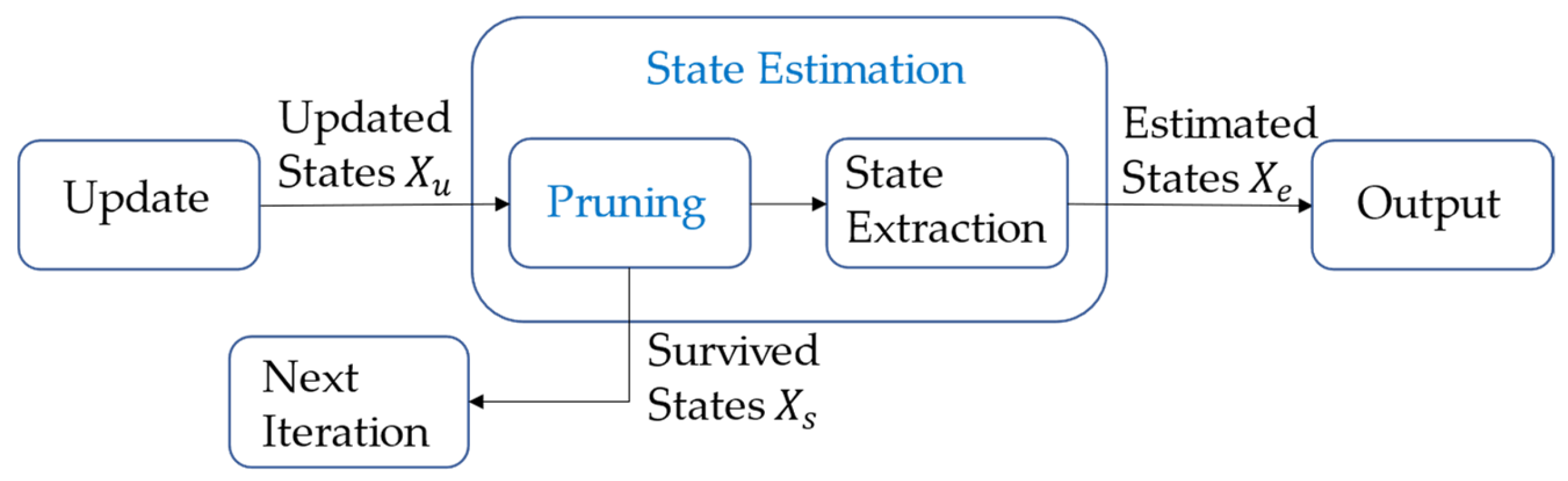
3.4. The Impact of Continuous Dynamic Clutter on State Estimation of LMB Filter

The state estimation stage mainly consists of two operations: trajectory pruning and state extraction. The mechanism for trajectory pruning is deleting trajectories whose existence probability is lower than the threshold, and other trajectories with higher existence probabilities are reserved for the next iteration:

$$\widehat{X}=\left\{\left(\widehat{x},\mathcal{l}\right):r^{\left(\mathcal{l}\right)}>\vartheta \right\}$$

(26)

where $\widehat{x}={\arg }_x\max p^{\left(\mathcal{l}\right)}\left(x\right)$.

The cardinality distribution, which is given by (10), provides the estimated target cardinality $N$, which is also the target number estimated by the LMB. States whose existence probability $r$ ranked at the top $N$ are extracted as estimated states.

The cardinality $N$ is calculated according to the existence probability $r$ and weight $w$, which are related to the posterior density in the update stage, according to (10) and (22). This is why unsuitable clutter intensity causes cardinality bias and further influences the tracking performance.

By comparing the differences in the spatial distribution of adjacent frames, the LMB filter can distinguish real-target trajectories from NCDC, but it can rarely do so from CDC. The challenges of inaccurate target number estimates can thus be addressed from the multipath propagation geometric characteristics (state-dependent characteristics) of CDC and the difference in the spatial distribution characteristics of longer frame sequences. Therefore, the hybrid clutter model LMB filter (HCM-LMB filter), which combines the characteristics of CDC and NCDC, is proposed based on the clutter model of the LMB filter that already conformed with the characteristics of NCDC.

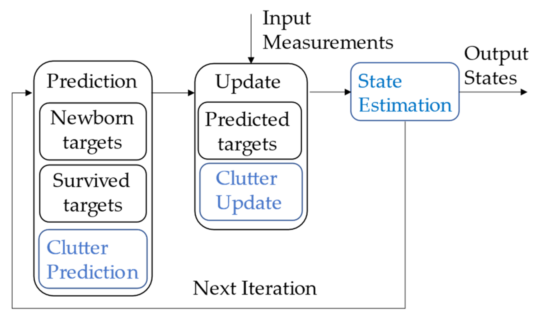
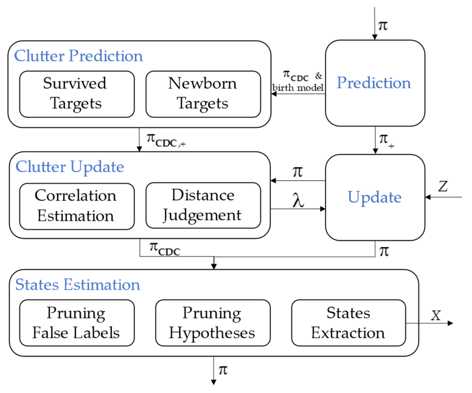
4. Hybrid Clutter Model LMB Filter

Based on the characteristics of the clutter model construct, the HCM-LMB filter aims to distinguish CDCs from real-target trajectories, thus reducing false trajectories caused by CDCs. The HCM-LMB filter’s prediction and update stages are the same as those of the LMB filter. However, the HCM-LMB filter also adds clutter prediction and update mechanisms, as well as a false trajectories management mechanism, to obtain a more accurate clutter estimation. The HCM-LMB filter changes the clutter intensity from a priori information to time-varying during the update stage. As a result, this section does not concentrate on the same parts that both the HCM-LMB filter and the LMB filter implement, instead emphasizing the hybrid clutter model and the newly added method for clutter prediction and update.

The framework of the HCM-LMB filter is depicted in Figure 4. It synchronously predicts and updates the clutter intensity, while the LMB filter predicts and estimates target states. In the clutter prediction stage, clutter intensity is simultaneously predicted during the LMB filter prediction based on the prior information from the previous iteration and the birth model. In the clutter estimation stage, the clutter intensity is updated based on the historical states of the target in each hypothesis and associated observations. In addition, the HCM-LMB filter adds a label space $\mathbb{F}$ of false trajectories to manage all potential false targets.

Accurate clutter intensity will act to obtain a more accurate posterior density, and thus improve the filter performance. The spatial distribution and mean value of the clutter are related to the calculation of clutter intensity. Therefore, it is necessary to combine the characteristics of dynamic clutters to estimate the clutter intensity.

The clutter model in the LMB filter is matched more closely to the NCDC’s characteristics; however, the CDC sequence’s characteristics are similar to a moving target trajectory, making it simple to be estimated as a target trajectory. To reduce the bias of the target number estimation, the clutter model of the LMB filter must be improved. Based on the clutter characteristics observed in Section 2, the clutter observation in the HCM-LMB filter is defined as:

• Time-varying: clutter is a Poisson point process, but the intensity is time-varying.
• Continuity: CDC sequences’ detection rates are no higher than their corresponding sequences generated from the same moving targets.
• Correlation: CDC is a clutter that is correlated with the moving target states, but they are independent of each other.
• Spatial distribution characteristics: the distance of CDC is always greater than the distance of its corresponding target state.

Non-continuous dynamic clutter, $C_{NCDC}$, is a Poisson point process with a mean value of ${\lambda }_{NCDC}$, and its spatial distribution, $c_{NCDC}\left(z\right)$, is assumed to be uniform in the field-of-view range. Continuous dynamic clutter, $C_{CDC}\left(X\right)$, is a Poisson point process with a clutter rate of ${\lambda }_{CDC}\left(X\right)$, and a spatial distribution of $c_{CDC}\left(z\left|X\right.\right)$, and its spatial distribution is assumed to be Gaussian with respect to the spatial state of its corresponding target. The static clutter of the three types of clutter is easily removed by the velocity characteristics of the point cloud, and the other two types of clutter, CDC and NCDC, are the main forms of clutter that need to be estimated. The average clutter rate is accumulated from the clutter rates of CDC and NCDC, as described in Equation (28). However, the final clutter rate and the spatial distribution of the clutter together contribute to the computation of the clutter intensity, as described in Equation (27), which in turn leads to a more accurate state update and target number estimation of the filters, as described in Equations (10), (20), and (25). The subscript “CDC” is used to denote the variables associated with CDC, and the subscript “NCDC” denotes the variables associated with NCDC. Therefore, the intensity function of the composite clutter process is:

$$k\left(Z,X\right)={\displaystyle \prod _{z\in Z}\lambda \left(X\right)c\left(z|X\right)}$$

(27)

where,

$$\lambda \left(X\right)\triangleq {\displaystyle \sum _{i=1}^n{\lambda }_{CDC}\left(x_i\right)+{\lambda }_{NCDC}},$$

(28)

$$c\left(z|X\right)\triangleq \frac{{\lambda }_{NCDC}{c}_{NCDC}\left(z\right)+{\displaystyle \sum _{i=1}^n{\lambda }_{CDC}\left(x_i\right)c_{CDC}\left(z|x_i\right)}}{{\displaystyle \sum _{i=1}^n{\lambda }_{CDC}\left(x_i\right)+{\lambda }_{NCDC}}},$$

(29)

according to the proof of the derivation of the measurement equation for the state-dependent false alarms in [18].

It is worth noting that the estimated states in the output of the LMB filter are not equivalent to the survived states in the next iteration. The relationship between the updated state set $X_u$, the survived state set $X_s$, and the estimated state set $X_e$ is shown in Figure 5, and the relationship between the three satisfies $X_e\subseteq X_s\subseteq X_u$. Therefore, the false state set $X_f$ will be used later to describe the updated state sets that are not output in this iteration, i.e., $X_f=X_u\cap \neg X_e$. The target trajectory related to the false-target states is regarded as a potential false target and will be assigned a false label, $f$, in the label space $\mathbb{F}$ of false targets.

The next section provides a detailed explanation of the HCM-LMB filter’s clutter prediction, clutter update, and false-track label management methods.

4.1. Clutter Prediction

The LMB filter processes the targets as newborn targets and survived targets in the prediction stage, then processes them in parallel in the subsequent stages. However, the update of clutter needs to use the historical states of the targets, and there is a significant difference in the number of historical states of the newborn and survived targets. In the stage of clutter update, the false trajectories generated by the CDC sequence are separately estimated as newborn false tracks and survived false tracks, i.e., the average rate of CDC is:

$${\lambda }_{CDC}\left(\mathrm{X}\right)={\lambda }_{CDC,B}\left(\mathrm{X}\right)+{\lambda }_{CDC,S}\left(\mathrm{X}\right)$$

(30)

where ${\lambda }_{CDC,B}\left(\mathrm{X}\right)$ is the CDC rate generated by the birth model, and ${\lambda }_{CDC,S}\left(\mathrm{X}\right)$ is the CDC rate of false trajectories in survived targets.

In the clutter prediction stage, the clutter rate is predicted based on the prior clutter rate and the birth model. The birth model produces Gaussian components in the prediction stage at time k, identified by the label: $\mathcal{l}=(k,i),\mathcal{l}\in \mathbb{B}$, where $i$ is the index. The newborn CDC average rate, ${\lambda }_{CDC,B}\left(\mathrm{X}\right)$, is predicted based on the number of birth components, and the survived CDC average rate, ${\lambda }_{CDC,S}\left(\mathrm{X}\right)$, is predicted based on the average clutter rate estimated in the last iteration, so the predicted clutter average rate, ${\lambda }_{CDC,+}\left(\mathrm{X}\right)$, is given by:

$$\begin{array}{l}{\lambda }_{CDC,+}\left(\mathrm{X}\right)={\lambda }_{CDC,B}\left(\mathrm{X}\right)+{\lambda }_{CDC,S}\left(\mathrm{X}\right)\\ \hspace{1em}\hspace{1em}=N_B+p_C\left(\mathrm{X}\right)\cdot {\lambda }_{k-1}\end{array}$$

(31)

where $N_B$ is the number of birth components, $p_C\left(\mathrm{X}\right)$ is the detection rate of the CDC sequence, and ${\lambda }_{k-1}$ is the average clutter rate estimated at time $k-1$.

4.2. Clutter Update

Since the clutter model of the HCM-LMB filter takes into consideration the characteristics of the CDC, it modifies the form of the observation model compared to the LMB filter.

For a given predicted target state set: $X=\left\{x_1,x_2,\dots ,x_n\right\}$, the observation set $Z$ of the HCM-LMB filter includes the target observation set $Z\left[T\left(X\right)\right]$ generated by the target direct wave and the clutter observation set $C\left(X\right)$, and the observation model is of the form:

$$Z=Z\left[T\left(X\right)\right]{\displaystyle \cup C\left(X\right)}$$

(32)

where the moving target observation is as in Equation (18), and the clutter observation set $C\left(X\right)$ contains the NCDC set $C_{NCDC}$ and the CDC set $C_{CDC}\left(X\right)$, which is given by:

$$C\left(X\right)=C_{NCDC}{\displaystyle \cup C_{CDC}\left(x_1\right){\displaystyle \cup \dots {\displaystyle \cup C_{CDC}\left(x_n\right)}}}$$

(33)

In the clutter update stage, the intensity of clutter measurements, $k\left(\cdot \right)$, utilized in (25), takes the following form:

$$k\left(Z,X;\mathsf{\theta }\right)=\lambda \left(Z,X\right)\cdot c\left(z_{\mathsf{\theta }\left(\mathcal{l}\right)}\left|X\right.\right)$$

(34)

According to the adaptive birth model, newborn targets are driven by measurement; thus, the measurement should be connected to updating the newborn continuous clutter rate, ${\lambda }_{CDC,B}\left(Z,X\right)$, and the clutter rate $\lambda \left(Z,X\right)$, as follows:

$$\lambda \left(Z,X\right)=\left\{\begin{array}{c}{\lambda }_{CDC,B}\left(Z\right)+{\displaystyle \prod _{i\in \mathbb{F}}\left(1-w_{CDC}\left(X,X^{\prime }\right)\right)}\cdot {\displaystyle \sum _{L\in {\mathcal{F}}_n\left(\mathbb{F}\right)}{\displaystyle \prod _{\mathcal{l}\in F}\frac{w_{CDC}\left(X,X^{\prime }\right)}{1-w_{CDC}\left(X,X^{\prime }\right)}}}+{\lambda }_{NCDC},if\left|Z\right|\ne Ø,\\ {\lambda }_{CDC,+}\left(X\right)+{\lambda }_{NCDC},if\left|Z\right|=Ø.\end{array}\right.$$

(35)

where,

$${\lambda }_{CDC,B}\left(Z\right)={\displaystyle \sum _{z\in Z}{\displaystyle \sum _{j=1}^{N_B}\neg {\mathrm{l}}_{S_{\mathsf{\alpha },j}}(z)}\cdot \left[1-f_{Gaus,j}\left(\left|z-{\overline{x}}_{B,j}\right|\right)\right]},$$

(36)

$$w_{CDC}\left(X,X^{\prime }\right)=\frac{{\rho }_{X{X}^{\prime }}\cdot p_D\left(X^{\prime }\right)}{p_D\left(X\right)},$$

(37)

where $S_{\mathsf{\alpha }}$ represents the birth area of the Gaussian confidence ellipse generated from the Gaussian birth components or distributions, with a confidence level of $1-\mathsf{\alpha }$. ${\mathrm{l}}_{S_{\mathsf{\alpha }}}(Z)$ denotes the inclusion relationship between the measurement and the birth area, $S_{\mathsf{\alpha }}$, $f_{Gaus}\left(\cdot \right)$ denotes the Gaussian probability density function of a Gaussian distribution in the birth model, ${\overline{x}}_B$ is the expected number of the Gaussian birth distribution, $w_{CDC}\left(X,X^{\prime }\right)$ represents the relevance weight, which is an application of correlation and continuity in the clutter model, and ${\rho }_{X{X}^{\prime }}$ denotes the Pearson correlation coefficient of a pair of random variables $\left(X,X^{\prime }\right)$.

4.3. Management of False Labels

The label space $\mathbb{L}$ of the predicted targets of the LMB filter consists of the label space ${\mathbb{L}}_{+}$ of the newborn targets at time $k$ and the label space $\mathbb{B}$ of the survived targets at time $k-1$, i.e., ${\mathbb{L}}_{+}=\mathbb{B}\cup \mathbb{L}$. In the scenario studied in this paper, the false label and its management mechanism are added based on the original label space, which means a trajectory may have both label $\mathcal{l}$ in label space $\mathbb{L}$ and false label $f$ in false label space $\mathbb{F}$. Since the filter copes well with NCDC, and CDC is the main reason why the filter fails to recognize and causes bias in the estimation of the number of targets, false labels are mainly used to mark false trajectories that may be caused by CDC.

If the state $x$ relates to a false label $f=Ø$, the state is considered not possible to be a false alarm caused by CDC. If $f\ne Ø$, the state $x$ is considered possible to be a false alarm caused by CDC, and its false label $f=\left(k,i\right),f\in \mathbb{F}$ relates to the track with the label $\mathcal{l}=\left(k,i\right),\mathcal{l}\in \mathbb{L}$. This correspondence, established by the false label, facilitates the quick identification of its corresponding target in the update stage. The trajectories with false labels that are not null also have states:

$${\mathsf{\pi }}_{CDC}=w_{CDC}{}^{\left(f\right)},f\in \mathbb{F}$$

(38)

where $w_{CDC}$ is given by (37) and (38).

Since a moving target may cause target observations and dynamic clutter observations, $\mathbb{F}\to \mathbb{L}$ is a single-shot, non-full-shot or double-shot relationship. The correspondence between states related to direct and multipath reflections from the same target is denoted by an apostrophe (‘), e.g., $X^{\prime }{}_{{\mathcal{l}}_1\in \mathbb{L},f_1\in \mathbb{F}}^{\left({\mathcal{l}}_1,f_1\right)}\to X_{{\mathcal{l}}_2\in \mathbb{L}}^{\left({\mathcal{l}}_2\right)}$, where $f_1\to {\mathcal{l}}_2$ is abbreviated as $X^{\prime }\to X$.

The construction of false labels occurs with hypotheses of both newborn and survived targets, and the principle of the construction is that all trajectories that may be false should be labeled with the false label $f\in \mathbb{F}$, with its relevance weight $w_{CDC}\left(X,X^{\prime }\right)$. The mechanisms of false label construction are different between newborn and survived hypotheses. The workflow scheme of clutter estimation in the HCM-LMB filter is shown in Figure 6.

For newborn hypotheses, they are generated by the birth model. In the stage of clutter prediction, every newborn hypothesis is considered as a false target, which means it is labeled with an original false label $f$. Therefore, the predicted clutter rate is also related to the number of birth components, which is also described in Equation (31).

In the stage of clutter update, the false labels and relevance weights are updated according to measurement set $Z$. As described in Equation (35), if there is no measurement, the newborn hypotheses gain a high probability of being a false target, and the false label $f$ will be kept. If any measurement, $z$, locates in any birth confidence region, $S_{\mathsf{\alpha }}$, of a birth hypothesis, the newborn hypothesis related to the measurement will not be considered as a false target, and its false label $f$ will be set as null. If any measurement conversely locates outside all birth confidence regions, the newborn hypothesis related to the measurement will increase the clutter rate, as described in Equation (37), and its false label $f$ will be kept. The newborn hypothesis with the original false label $f$ will be related to the survived hypothesis that is closest to it in spatial distribution.

For survived hypotheses, hypotheses without false labels are compared to each other via the historical spatial distribution of states, and if there is a hypothesis satisfying the condition that all its states’ distances are greater than a corresponding hypothesis, a false label $f\in \mathbb{F}$ is constructed for it. This is performed in accordance with the spatial distribution characteristics of the CDC model.

In the states’ extraction stage, the HCM-LMB filter prunes the trajectories with an existence probability below a certain threshold, and removes the false labels by nulling certain trajectories whose relevance weights, $w_{CDC}\left(X,X^{\prime }\right)$, are below the threshold or whose updated spatial states do not satisfy the condition that the distance is greater than that of their corresponding trajectories.

5. Experiments and Analysis

5.1. Experimental Data

The experimental scenario was based in a lobby that connected to a corridor with three elevator entrances. Pedestrians were collected by the radar when they passed through the lobby, as shown in Figure 7a. The appearing and disappearing locations included the right corridor and the three elevator entrances. The scenario’s plan view with the radar scanning range and a coordinate system is shown in Figure 7b. The scanning distance of the millimeter-wave radar can reach up to 250 m, which is much further than the farthest distance of the field-of-view. The figure only shows the coverage capability of the radar in this specific scenario, where the radar covered the lobby almost completely.

The experimental system consists of two main devices: a 77 GHz 2D millimeter-wave radar and a camera. Both devices were fixed on a tripod, and the radar was connected to a computer and transmitted data through a CAN interface, as shown in Figure 8. The radar used in the experimental system is Continental’s ARS408-21 FMCW (Frequency-Modulated Continuous Wave) radar, with its data sheet as shown in

Table 1. Data sheet of the millimeter-wave radar.

Measuring Performance	Value
Data rate	17 Hz
Antenna channels	4TX/2x6RX
Accuracy of distance measurement	$\pm$0.1 m
Distance range	0.20 m to 250 m
Accuracy of azimuth angle	$\pm$0.1°
Range of azimuth angle	−60° to 60°

. The image data captured by the camera were solely used for distinguishing targets and confirming the target number, which served as the foundation for a later evaluation of the accuracy of the filter’s target number estimation.

There were 22 sets of data collected in the scenario depicted in Figure 8, which were used in the following experiments. Section 5.2 details the verification of the consistency between the real data and the characteristics model of the two dynamic clutters analyzed in Section 2. In Section 5.3, two typical sets of data, which contain both CDC and NCDC, are used to evaluate the pedestrian counting and tracking performance of HDBSCAN, the HCM-LMB filter, and the LMB filter. Then, the pedestrian counting and tracking performance of the 3 algorithms applied to the 22 sets of data are also measured.

5.2. Clutter Characteristics Model Validation with Real Data

A typical set of data that includes both NCDC and CDC caused by radar indoor multipath scattering was collected for analysis in the scenario shown in Figure 9 and used to validate the characteristics of the clutters. As shown in Figure 9, points in different colors were processed by HDBSCAN [9], having been sieved for static clutter by velocity limitation, where the red and blue sequences were considered by HDBSCAN as two different clusters and the black sequences were considered as outliers. The outliers were considered as non-continuous dynamic clutter since they both showed the same characteristics.

From Figure 9, the distance of the CDC sequence was larger than that of its related moving target sequence. In addition, the geometric correspondence between the CDC sequence and the moving target sequence can be observed more visually in the spatial distribution, as shown in Figure 10.

The Pearson correlation coefficients, $\rho$, shown in Equation (5) and the detection rates, $p_D$, were calculated to verify the sequence correlation and continuity of clutter and targets in the above data. The results are shown in

Table 2. Detection rate and continuity evaluation.

Sequence	Detection Probability, ${\mathit{p}}_{\mathit{D}}$	Range–Angle Correlation Coefficient, ${\mathit{\rho }}_{\mathit{R}\mathit{A}}$	Time–Range Correlation Coefficient, ${\mathit{\rho }}_{\mathit{T}\mathit{R}}$	Time–Angle Correlation Coefficient, ${\mathit{\rho }}_{\mathit{T}\mathit{A}}$
Continuous dynamic clutter	0.800	0.158	0.898	0.245
Moving target 1	0.900	0.682	0.897	0.876
Non-continuous dynamic clutter	0.111	−0.166	0.977	−0.341
Moving target 2	1.000	0.691	0.976	0.762

, which contains a CDC sequence, a NCDC sequence, and their related moving target sequences. The CDC sequence corresponds to the moving target sequence 1 and its occurrence time is 42–51 frames, and the NCDC sequence corresponds to the moving target sequence 2, with an occurrence time of 25–87 frames.

From the above results, both the CDC sequence and the moving target sequences showed high continuity, but the continuity of the NCDC sequence was lower. As shown in Figure 6, the point cloud of CDC was sparser compared to the point cloud of the moving target. Therefore, the difference in the detection rates can be used to distinguish the two kinds of clutter sequences and their moving target sequences.

The time-distance correlation coefficient, ${\mathsf{\rho }}_{TR}$, of the CDC sequence was similar to that of the moving target sequence, but the distance-angle correlation coefficient, ${\mathsf{\rho }}_{RA}$, and time-angle correlation coefficient, ${\mathsf{\rho }}_{TA}$, were different from that of the moving target sequence. It is speculated that this may be caused by the multipath wave of the radar on both sides of the moving target and the generated sequences, which made the angular uncertainty increase and the variance become larger. While the angular resolution of the millimeter-wave radar is lower, the multipath effect on the angular characteristics distinguishes the CDC sequence from the moving target sequence. Therefore, the time-distance correlation coefficient, ${\mathsf{\rho }}_{TR}$, can also be used to distinguish the two kinds of clutter sequences and the moving target sequences.

5.3. Performance Evaluation in Pedestrian Counting and Tracking

To evaluate the performance of the HCM-LMB filter in counting pedestrians and tracking, the LMB filter was implemented with the same parameters as the HCM-LMB filter in two scenes as a comparison. In scenes A and B, the observed CDCs were generated after or along with the birth of their related moving targets, causing different degrees of complexity to the filters. The moving targets in the two scenes appeared or disappeared from different locations in the field-of-view.

Generally, the target point cloud generated by the millimeter-wave radar is extended target data. However, quite a lot of the collected moving target data appear as point target data, due to the small field-of-view of the experimental scene, the low radar accuracy, and occlusions of targets. In order to fit the assumption of the LMB filter that the target is a point target, pre-processing of raw data is necessary.

The processing flow of the experimental data is shown in Figure 11. The raw point cloud data captured by the 2D millimeter-wave radar were first restricted by the velocity information, which was removed from the static noise, and then the dynamic point cloud data were obtained. After being pre-processed by a clustering method, the dynamic point cloud data were used for tracking and target number estimation.

The pre-processing was based on the principle that the detection rate and approximate spatial distribution of the moving target and CDC sequences were not affected as much as possible, and a simple HDBSCAN clustering process was performed on the experimental raw data. In the process of clustering, two or more points with very high spatial similarity among the denser clusters in each frame were combined into one point by taking the mean value. The outliers estimated by HDBSCAN were kept, as they showed the same characteristics as the NCDCs.

The LMB and HCM-LMB filters in scenes A and B both implement a Gaussian mixture solution. In scene A, three targets approached the radar and one was moving away, and CDC was observed on one side of one of the approaching targets and on both sides of the leaving target.

Figure 12 shows the results estimated by the LMB filter, the HCM-LMB filter, and HDBSCAN in scene A, where the two filters had the same prior and filter parameters. The prior detection rate, $p_D$, was 0.75, the prior clutter intensity, $\lambda$, was 1.5, and there were two Gaussian components in the birth model, which means it produces two newborn targets at the prediction stage in each iteration.

HDBSCAN is a hierarchical density-based clustering method and can separate clusters with different densities. The parameters of HDBSCAN in Figure 12 include a cluster selection epsilon of 0.052 and a minimum sample size of 3.

The false trajectories estimated by the LMB filter are marked by black boxes in Figure 12a, where HDBSCAN also estimated false-target trajectories in the region. The trajectories are marked by the black and red boxes in Figure 12e, where two of the approaching trajectories were also estimated by HDBSCAN as one target. This may be because the clutters in the middle of the two trajectories made the point clouds of the two trajectories reachable, and the two trajectories were mistakenly considered as the same target. The trajectories mentioned in Figure 12c were more accurately estimated by the HCM-LMB filter, although there were a few assignment errors.

The green boxes in Figure 12a,e mark a fragmented trajectory with ID switches of trajectories. The possible reasons are the high local missed detection rate of the trajectory and the uneven distribution of clutter. However, the HCM-LMB filter in Figure 12c did not estimate false trajectories in this region, and the degree of trajectory fragmentation was reduced. All three algorithms are capable of handling NCDCs well and do not estimate false trajectories caused by NCDCs, but occasionally, NCDCs have an impact on the two filters’ assignment of measurement, which can reduce the tracking accuracy.

The tracking results of the three algorithms in scene B are shown in Figure 13. In scene B, the CDC sequence appeared almost simultaneously with the pedestrians and lasted longer than that in scene A, and the missed detection rate was higher. In scene B, three targets approached the radar and one was moving away. Two of the approaching targets were occluded and showed a high missed detection rate, and a more complex CDC was observed near the distant target.

Figure 13 shows the results estimated by the LMB filter, the HCM-LMB filter, and HDBSCAN in scene B, where the two filters had the same prior and filter parameters. The prior detection rate, $p_D$, was 0.8, and the prior clutter intensity, $\lambda$, was 2. There were also two Gaussian components in the birth model. The parameters of HDBSCAN in Figure 13 include a cluster selection epsilon of 0.4 and a minimum sample size of 4.

The black boxes in Figure 13a,e mark false trajectories caused by CDCs that do not appear in Figure 13c, in the results estimated by the HCM-LMB filter. Additionally, in comparison to HDBSCAN, the LMB filter can deal with CDCs with a high missed detection rate without mistaking them as false targets. The green box in Figure 13e marks two target trajectories in the region; however, they were mistakenly considered as the same target trajectory by HDBSCAN, and there were also false trajectories. In Figure 13c, the HCM-LMB filter accurately estimated the total number of targets, although some of the trajectories exhibited a certain rate of missed detection, which may also be related to the occlusion between targets. The NCDCs also did not affect the target number estimation of the three algorithms in scene B but they did influence the observation point assignment of the two filters.

The cardinality estimation with time for the LMB filter, the HCM-LMB filter, and HDBSCAN in scenes A and B is shown in Figure 14a,b, respectively. The bias of the HCM-LMB filter for the target number estimation was more accurate compared to the LMB filter and HDBSCAN.

Table 3. Performance evaluation based on data of scenes A and B.

Scene	Evaluation Indicators	LMB Filter	HCM-LMB Filter	HDBSCAN
Scene A	Number bias of pedestrians	4	1	7
	MOTA	0.669	0.819	0.666
	Total cardinality bias	58	37	36
	False positives	47	5	18
	False negatives	11	32	18
Scene B	Number bias of pedestrians	1	0	3
	MOTA	0.812	0.829	0.518
	Total cardinality bias	44	42	72
	False positives	21	2	10
	False negatives	23	40	62

lists the evaluation of the cardinality estimation and tracking accuracy of the above results. The number bias of pedestrians, total cardinality bias, total missed detections (false negatives), and total false alarms (false positives) in all frames were used as evaluation indicators. The true value of the target number was obtained by manually discriminating the data collected by the camera in the experimental system. The cardinality bias measures the ability of the algorithm to identify the targets by the label number of the trajectories, which is calculated as shown in Equation (39). The total number of missed detections and false alarms in all frames accumulate the number of missed detections and false alarms per frame, which measures the accuracy of the algorithm’s cardinality estimation. Tracking accuracy was evaluated using multiple-object tracking accuracy (MOTA) [34], which incorporates the three issues of missed detection, false alarm, and target ID retention into the measure, and the higher its value, the higher the tracking accuracy.

$$Bias=\left|\left|{\mathbb{L}}_{est}\right|-N_{true}\right|$$

(39)

where $\left|{\mathbb{L}}_{est}\right|$ denotes the cardinality of the label space of the algorithm-estimated state, i.e., the number of pedestrians estimated by the algorithm, and $N_{true}$ denotes the number of real moving targets, i.e., the true number of pedestrians.

According to Table 3, compared to HDBSCAN, the HCM-LMB filter performed better in pedestrian number bias, MOTA, and false alarms/false positives, and performed better or comparable to HDBSCAN in the total cardinality bias. The HCM-LMB filter showed higher missed detections/false negatives in scene A and lower missed detections in scene B. Compared to the LMB filter, the HCM-LMB filter performed better in pedestrian number bias, MOTA, total cardinality bias, and false alarms, but showed higher missed detections. In total, the HCM-LMB filter reduced the total cardinality bias by 22.5% and 26.9% compared to the LMB filter and HDBSCAN, respectively, for a total of 270 frames in both scenes.

The worse performance of the HCM-LMB filter in missed detections is related to the fact that the measurements showed a certain rate of missed detections. At some point, the false alarms of HDBSCAN and the LMB filter compensated for the missed detections, making HDBSCAN and the LMB filter perform better than the HCM-LMB filter in missed detections.

To further evaluate the performance of the HCM-LMB filter, a total of 1046 frames of data processed by the LMB filter and the HCM-LMB filter were statistically evaluated and analyzed with the following indicators: average missed detection rate, false-alarm rate, MOTA, and average number bias of pedestrians. As shown in

Table 4. Performance evaluation based on data.

Evaluation Indicators	LMB Filter	HCM-LMB Filter
Average number bias of pedestrians	2.4	0.8
MOTA	0.858	0.902
Missed detection rate	7.6%	8.6%
False-alarm rate	8.1%	1.9%

, although the HCM-LMB filter still had a larger missed detection rate, it not only improved its performance in counting pedestrians by reducing the pedestrian number bias, but it also reduced the false-alarm rate, subsequently affecting the tracking accuracy performance in the closed-space scenario.

6. Conclusions

In this paper, we addressed the problem of target number estimation bias caused by the multipath effect of the LMB filter when the millimeter-wave radar is utilized to monitor pedestrians. First, we analyzed the millimeter-wave radar point cloud data collected from closed scenes for spatial and spatial–temporal distribution characteristics and classified and modeled the clutters into three classes: static clutter, NCDC, and CDC. Then, we proposed the hybrid clutter model labeled multi-Bernoulli (HCM-LMB) filter based on these clutter characteristics. Finally, as an experiment, we performed a statistical analysis on the detection rate and correlation of the data collected within an enclosed space. This analysis aimed to validate the alignment with the clutter characteristic model. Furthermore, a comparative evaluation was conducted between the performance of the HCM-LMB filter and both the LMB filter, utilizing identical parameters, and the HDBSCAN method. The results demonstrated the efficacy of the HCM-LMB filter in reducing the target number estimation bias in enclosed spaces.

CDC was found as the main cause of bias in estimating pedestrian numbers. CDC shows similarity in characteristics to the point cloud of moving targets generated by the direct wave and differs from NCDC (outliers) in density and statistics. This similarity often leads to CDC being incorrectly estimated as a moving target, which biases the number of pedestrian targets. Thus, we proposed the HCM-LMB filter, using CDC’s dynamic clutter average rate during predictive density estimation, creating a CDC clutter intensity model, and adding a noise rate computation weight based on Pearson’s correlation coefficient during updating, which were all necessary to achieve this. The HCM-LMB filter improved the probability density estimated for CDC assumption states in the LMB. This ultimately mitigated the impact of CDC on the pedestrian target count estimation by effectively managing false labels.

The HCM-LMB filter proposed in this paper can more accurately estimate the number of targets under the multipath effect, but it also has a drawback of having a marginally higher probability of missed detection than the LMB filter, which will need to be addressed in the future. Regular walking was the type of pedestrian posture we observed in the experiment, but it is important to consider how running or other pedestrian posture changes would affect the filter, which is another issue to investigate in the future.

References

1. Zhou, T.; Yang, M.; Jiang, K.; Wong, H.; Yang, D. MMW radar-based technologies in autonomous driving: A review. Sensors 2020, 20, 7283. [Google Scholar] [CrossRef] [PubMed]
2. Zhou, Y.; Dong, Y.; Hou, F.; Wu, J. Review on Millimeter-Wave Radar and Camera Fusion Technology. Sustainability 2022, 14, 5114. [Google Scholar] [CrossRef]
3. Li, Y.; Wei, Y.; Wang, Y.; Lin, Y.; Shen, W.; Jiang, W. False Detections Revising Algorithm for Millimeter Wave Radar SLAM in Tunnel. Remote Sens. 2023, 15, 277. [Google Scholar] [CrossRef]
4. Cook, A.A.; Mısırlı, G.; Fan, Z. Anomaly Detection for IoT Time-Series Data: A Survey. IEEE Internet Things J. 2020, 7, 6481–6494. [Google Scholar] [CrossRef]
5. Ester, M.; Kriegel, H.P.; Sander, J.; Xu, X. A density-based algorithm for discovering clusters in large spatial databases with noise. kdd 1996, 96, 34. [Google Scholar]
6. Comaniciu, D.; Meer, P. Mean shift: A robust approach toward feature space analysis. IEEE Trans. Pattern Anal. Mach. Intell. 2002, 24, 603–619. [Google Scholar] [CrossRef]
7. Ankerst, M.; Breunig, M.M.; Kriegel, H.P.; Sander, J. OPTICS: Ordering points to identify the clustering structure. ACM Sigmod Rec. 1999, 28, 49–60. [Google Scholar] [CrossRef]
8. Zhang, T.; Ramakrishnan, R.; Livny, M. BIRCH: An efficient data clustering method for very large databases. ACM Sigmod Rec. 1996, 25, 103–114. [Google Scholar] [CrossRef]
9. Campello, R.; Moulavi, D.; Sander, J. Density-Based Clustering Based on Hierarchical Density Estimates in Advances in Knowledge Discovery and Data Mining; Springer: Berlin/Heidelberg, Germany, 2013; pp. 160–172. [Google Scholar]
10. Bhuyan, M.H.; Bhattacharyya, D.K.; Kalita, J.K. Network Anomaly Detection: Methods, Systems and Tools. IEEE Commun. Surv. Tutor. 2014, 16, 303–336. [Google Scholar] [CrossRef]
11. Zoubir, A.M.; Koivunen, V.; Chakhchoukh, Y.; Muma, M. Robust estimation in signal processing: A tutorial-style treatment of fundamental concepts. IEEE Signal Process. Mag. 2012, 29, 61–80. [Google Scholar] [CrossRef]
12. Ross, S.M. Peirce’s criterion for the elimination of suspect experimental data. J. Eng. Technol. 2003, 20, 38–41. [Google Scholar]
13. Blackman, S.S.; Popoli, R. Design and Analysis of Modern Tracking Systems; Artech House: Boston, MA, USA, 1999. [Google Scholar]
14. Fortmann, T.; Bar-Shalom, Y.; Scheffe, M. Sonar tracking of multiple targets using joint probabilistic data association. IEEE J. Ocean. Eng. 1983, 8, 173–184. [Google Scholar] [CrossRef]
15. Reid, D. An algorithm for tracking multiple targets. IEEE Trans. Autom. Control 1979, 24, 843–854. [Google Scholar] [CrossRef]
16. Mahler, R. Multitarget Bayes filtering via first-order multitarget moments. IEEE Trans. Aerosp. Electron. Syst. 2003, 39, 1152–1178. [Google Scholar] [CrossRef]
17. Vo, B.-N.; Ma, W.-K. The Gaussian mixture probability hypothesis density filter. IEEE Trans. Signal Process. 2006, 54, 4091–4104. [Google Scholar] [CrossRef]
18. Mahler, R. Statistical Multisource-Multitarget Information Fusion; Artech House: Norwood, MA, USA, 2007; Volume 685. [Google Scholar]
19. Ristic, B.; Clark, D.; Vo, B.-N.; Vo, B.-T. Adaptive Target Birth Intensity for PHD and CPHD Filters. IEEE Trans. Aerosp. Electron. Syst. 2012, 48, 1656–1668. [Google Scholar] [CrossRef]
20. Mahler, R. PHD filters of higher order in target number. IEEE Trans. Aerosp. Electron. Syst. 2007, 43, 1523–1543. [Google Scholar] [CrossRef]
21. Vo, B.-T.; Vo, B.-N.; Cantoni, A. Analytic Implementations of the Cardinalized Probability Hypothesis Density Filter. IEEE Trans. Signal Process. 2007, 55, 3553–3567. [Google Scholar] [CrossRef]
22. Vo, B.-T.; Vo, B.-N.; Cantoni, A. The Cardinality Balanced Multi-Target Multi-Bernoulli Filter and Its Implementations. IEEE Trans. Signal Process. 2009, 57, 409–423. [Google Scholar] [CrossRef]
23. Ristic, B.; Vo, B.-T.; Vo, B.-N.; Farina, A. A Tutorial on Bernoulli Filters: Theory, Implementation and Applications. IEEE Trans. Signal Process. 2013, 61, 3406–3430. [Google Scholar] [CrossRef]
24. Vo, B.-T.; Vo, B.-N. A random finite set conjugate prior and application to multi-target tracking. In Proceedings of the 2011 Seventh International Conference on Intelligent Sensors, Sensor Networks and Information Processing, Adelaide, SA, Australia, 6–9 December 2011; pp. 431–436. [Google Scholar] [CrossRef]
25. Vo, B.-T.; Vo, B.-N. Labeled Random Finite Sets and Multi-Object Conjugate Priors. IEEE Trans. Signal Process. 2013, 61, 3460–3475. [Google Scholar] [CrossRef]
26. Vo, B.-N.; Vo, B.-T.; Phung, D. Labeled Random Finite Sets and the Bayes Multi-Target Tracking Filter. IEEE Trans. Signal Process. 2014, 62, 6554–6567. [Google Scholar] [CrossRef]
27. Vo, B.-N.; Vo, B.-T.; Hoang, H.G. An Efficient Implementation of the Generalized Labeled Multi-Bernoulli Filter. IEEE Trans. Signal Process. 2017, 65, 1975–1987. [Google Scholar] [CrossRef]
28. Reuter, S.; Vo, B.-T.; Vo, B.-N.; Dietmayer, K. Multi-object tracking using labeled multi-Bernoulli random finite sets. In Proceedings of the 17th International Conference on Information Fusion (FUSION), Salamanca, Spain, 7–10 July 2014; pp. 1–8. [Google Scholar]
29. Reuter, S.; Vo, B.-T.; Vo, B.-N.; Dietmayer, K. The Labeled Multi-Bernoulli Filter. IEEE Trans. Signal Process. 2014, 62, 3246–3260. [Google Scholar] [CrossRef]
30. Suzuki, K.; Yamano, C.; Ikoma, N. Multiple Target Tracking in Automotive FCM Radar by Multi-Bernoulli Filter with Elimination of Other Targets. In Proceedings of the 2018 21st International Conference on Information Fusion (FUSION), Cambridge, UK, 10–13 July 2018; pp. 527–534. [Google Scholar] [CrossRef]
31. Fröhle, M.; Granström, K.; Wymeersch, H. Decentralized Poisson Multi-Bernoulli Filtering for Vehicle Tracking. IEEE Access 2020, 8, 126414–126427. [Google Scholar] [CrossRef]
32. Ishtiaq, N.; Gostar, A.K.; Bab-Hadiashar, A.; Palmer, J.; Hosseinezhad, R. Interaction-Aware Labeled Multi-Bernoulli Filter with Road Constraints. In Proceedings of the 2022 11th International Conference on Control, Automation and Information Sciences (ICCAIS), Hanoi, Vietnam, 21–24 November 2022; pp. 248–254. [Google Scholar] [CrossRef]
33. Ishtiaq, N.; Gostar, A.K.; Bab-Hadiashar, A.; Hoseinnezhad, R. Interaction-Aware Labeled Multi-Bernoulli Filter. Available online: https://arxiv.org/abs/2204.08655 (accessed on 19 April 2022).
34. Bernardin, K.; Stiefelhagen, R. Evaluating multiple object tracking performance: The clear mot metrics. EURASIP J. Image Video Process. 2008, 2008, 1–10. [Google Scholar] [CrossRef]
Figure 1. Simulation diagrams of dynamic clutters and the moving target, where black points represent non-continuous dynamic clutters, red points represent continuous dynamic clutters, and blue points represent observations of a moving target. (a) Spatial distribution of non-continuous dynamic clutter. (b) Spatial–temporal distribution of non-continuous dynamic clutter. (c) Spatial distribution of continuous dynamic clutter. (d) Spatial–temporal distribution of continuous dynamic clutter caused by radar indoor multipath scattering.
Remotesensing 15 04698 g001
Figure 2. Schematic diagram of continuous dynamic clutter caused by radar indoor multipath scattering.
Remotesensing 15 04698 g002
Figure 3. Scheme of the LMB filter.
Remotesensing 15 04698 g003
Figure 4. Scheme of the hybrid clutter model LMB filter, where parts in blue are those that distinguish the HCM-LMB filter from the LMB filter.
Remotesensing 15 04698 g004
Figure 5. Illustration of the relationship between updated states, survived states, and estimated states.
Remotesensing 15 04698 g005
Figure 6. The workflow scheme of clutter estimation in the HCM-LMB filter.
Remotesensing 15 04698 g006
Figure 7. Experimental scenario: (a) the experimental system capturing pedestrian data, and (b) the plan view with the radar scanning range.
Remotesensing 15 04698 g007
Figure 8. Experimental system: (a) the local details of 77GHz radar and camera, and (b) radar and camera are installed on a tripod.
Remotesensing 15 04698 g008
Figure 9. Spatial-temporal distribution of a single target moving away, where blue points represent measurement of the target, black points represent non-continuous dynamic clutter, and red points represent continuous dynamic clutter caused by radar indoor multipath scattering.
Remotesensing 15 04698 g009
Figure 10. Spatial distribution of continuous dynamic clutter–target measurement pairs, where blue points represent measurement of targets and red points represent continuous dynamic clutter, and each sequence is marked by a red circle.
Remotesensing 15 04698 g010
Figure 11. Overview of the data processing chain.
Remotesensing 15 04698 g011
Figure 12. Results plot of scene A, where dots with same color are states with same label or states in same trajectory and gray crosses are measurements. The green box marks the phenomenon of ID switch, the black box marks the phenomenon of false trajectories, and the red box marks the phenomenon of trajectory overlap or missed detection. (a) Two-dimensional view of the LMB filter’s spatial–temporal distribution result. (b) Three-dimensional view of the LMB filter’s spatial–temporal distribution result. (c) Two-dimensional view of the HCM-LMB filter’s spatial-temporal distribution result. (d) Three-dimensional view of the HCM-LMB filter’s spatial-temporal distribution result. (e) Two-dimensional view of HDBSCAN’s spatial–temporal distribution result. (f) Three-dimensional view of HDBSCAN’s spatial-temporal distribution result.
Remotesensing 15 04698 g012
Figure 13. Results plot of scene A, where dots with same color are states with same label or states in same trajectory and gray crosses are measurements. The green box marks the phenomenon of ID switch, the black box marks the phenomenon of false trajectories, and the red box marks the phenomenon of trajectory overlap or missed detection. (a) Two-dimensional view of the LMB filter’s spatial–temporal distribution result. (b) Three-dimensional view of the LMB filter’s spatial–temporal distribution result. (c) Two-dimensional view of the HCM-LMB filter’s spatial–temporal distribution result. (d) Three-dimensional view of the HCM-LMB filter’s spatial–temporal distribution result. (e) Two-dimensional view of HDBSCAN’s spatial–temporal distribution result. (f) Three-dimensional view of HDBSCAN’s spatial–temporal distribution result.
Remotesensing 15 04698 g013
Figure 14. Cardinality estimation: (a) estimated cardinalities in scene A, and (b) estimated cardinalities in scene B.
Remotesensing 15 04698 g014