Article

Weighted Maximum Correntropy Criterion-Based Interacting Multiple-Model Filter for Maneuvering Target Tracking

1
School of Electronics and Information, Northwestern Polytechnical University, Xi’an 710072, China
2
AVIC Leihua Electronic Technology Research Institute, Wuxi 214063, China
3
School of Automation Science and Engineering, Xi’an Jiaotong University, Xi’an 710049, China
*
Author to whom correspondence should be addressed.
Remote Sens. 2023, 15(18), 4513; https://doi.org/10.3390/rs15184513
Submission received: 2 August 2023 / Revised: 6 September 2023 / Accepted: 7 September 2023 / Published: 13 September 2023
(This article belongs to the Special Issue Advances in Radar Systems for Target Detection and Tracking)

Abstract

:
During the process of maneuvering target tracking, the measurement may be disturbed by outliers, which leads to a decrease in the state estimation performance of the classic interacting multiple-model (IMM) filter. To solve this problem, a weighted maximum correntropy criterion (WMCC)-based IMM filter is proposed. In the proposed filter, the fusion state is used as the input of each sub-model to reduce the computational complexity of state interaction and the WMCC is adopted to derive the sub-model state update and state fusion to improve the state estimation performance under outlier interference. Through principal analysis, the superiority of the proposed filter over the classic IMM filter in fusion strategy is revealed. The specific form of the proposed filter in radar maneuvering target tracking is provided. Two experimental cases of maneuvering target tracking are tested to illustrate the effectiveness of the proposed filter.

1. Introduction

The state estimation problem has received widespread attention because of its existence in various fields such as target tracking [1], navigation and positioning [2], and signal processing [3]. For target tracking, the state estimation is the most important step in its implementation process. When the maneuvering ability of the target is weak, its motion characteristics can be modeled by using the constant velocity (CV) model [4] or the constant turn (CT) model [5]. The Kalman filter (KF) or the extended Kalman filter (EKF) can be used to solve its state estimation problem. The KF is an optimal Bayesian state estimator of the single-model linear system in the Gaussian noise environment [6,7,8], and the EKF is an approximate KF applied to the single-model nonlinear system. Both of these filters assume that the process noise and the measurement noise follow the Gaussian distribution, which means that the estimation performance of both filters will decrease in the non-Gaussian noise environment.
When the target has strong maneuverability, the single model methods have limited estimation ability and the multiple model methods need to be used for state estimation. Unfortunately, the optimal filter for a multiple-model linear system does not exist because the computational process of analytical solutions is very difficult. As a pseudo-Bayesian sub-optimal algorithm, the interactive multiple-model (IMM) filter [9,10,11] is the most frequently used approach to solve the problem of multiple-model state estimation. Similar to the KF and EKF, the classic IMM filter [9,10,11] also models the noise as the Gaussian distribution, which also causes its estimation performance to deteriorate under the non-Gaussian noise.
In practical applications, due to the low cost and instability of the sensor, the measurement is susceptible to outliers, which leads its noise to follow the non-Gaussian distribution. To improve the robustness, some filters based on the variational Bayesian (VB) method are proposed, such as the IMM-VB filter, the Gaussian–Pearson type VII mixture model-based robust VB-KF, and the inverse gamma model and generalized hyperbolic skew Student’s t model-based VB-KF [12,13,14]. Although the IMM-VB filter can effectively improve the state estimation accuracy of the multiple-model system under a non-Gaussian measurement noise environment, the computational burden is large, and an accurate non-Gaussian noise model needs to be required. Recently, a maximum correntropy criterion (MCC) method [15] has been widely used to solve the problem of state estimation under outlier interference. Compared with the VB, the MCC has higher computational efficiency and does not need an accurate noise model. To solve the problem of state estimation under outlier interference, the MCC-based KF (MCCKF) [16], cubature Kalman filter (MCCCKF) [17], and unscented Kalman filter (MCCUKF) [18] are successively proposed. Based on these filters, Ref. [19] proposes an improved MCCCKF, which can adaptively estimate the kernel bandwidth to improve the positioning performance of a cooperative localization system. Ref. [20] proposes an improved MCCUKF to overcome the problem of numerical instability under large shot noise, and Ref. [21] proposes a distributed MCCKF to improve estimation performance in the presence of impulsive noise. In addition, a novel MCC-based Rauch–Tung–Striebel smoother [22] is proposed to solve the state estimation problem under non-Gaussian process and measurement noises. For the maneuvering target tracking, the multiple-model-based filter is currently the mainstream method [23,24,25]. Unfortunately, the above MCC-based filters are designed based on a single model, and they cannot solve the multiple-model state estimation problem under outlier interference. How to design multiple-model filters based on the maximum entropy criterion to improve the state estimation accuracy of maneuvering targets under outlier interference needs to be solved.
Currently, an MCC-based filter, which is called the IMM-MCC filter [26], is designed based on the multiple model, and this filter can be considered as a combination of the IMM filter and MCCKF. To further improve the state estimation accuracy of a maneuvering target under outlier interference, a weighted MCC-based IMM (WMCC-IMM) filter is proposed. The proposed filter is also designed based on the multiple model. The main contributions of this article are as follows.
(1)
Different from the IMM-MCC filter, the proposed filter adopts another Gaussian kernel function [20] to construct the cost function. Based on this Gaussian kernel function, the weighted maximum correntropy criterion is defined, and a new cost function is given.
(2)
The sub-model state update and state fusion steps are derived under the framework of WMCC, and the previous fusion state is used as the input of each sub-model to simplify the state interaction step.
(3)
The difference between the IMM-MCC filter and WMCC-IMM filter is discussed, which reveals the superiority of the proposed filter in fusion strategy.
(4)
To solve the state estimation problem of a maneuvering target in a radar system, the specific steps of the WMCC-IMM filter in radar maneuvering target tracking is given.
(5)
The effectiveness of the WMCC-IMM filter is tested using a set of simulation data and a set of actual test data. Simulation results show that the WMCC-IMM filter has better state estimation performance than the IMM-MCC filter. The great feedback from actual test data indicates that the proposed filter has potential value for practical engineering applications.
The structure of this article is as follows. In Section 2, the problem under consideration is formulated, and the IMM filter is introduced. In Section 3, the main results are presented, where the WMCC is defined, the WMCC-IMM filter is derived, the difference between the IMM-MCC filter and WMCC-IMM filter is discussed, and the specific steps of the WMCC-IMM filter in radar maneuvering target tracking is given. In Section 4, two maneuvering target tracking cases are tested to verify the effectiveness of the WMCC-IMM filter. Lastly, the conclusion is drawn in Section 5.

2. Problem Formulation

The discrete linear multiple-model system at time k + 1 can be represented by the following equations:
x k + 1 = F k i x k + w k i
z k + 1 = H k + 1 i x k + 1 + v k + 1 i
where Equations (1) and (2) are the state transition equation and measurement equation, respectively. x k + 1 n × 1 and z k + 1 m × 1 represent the state vector and measurement vector, respectively. F k i n × n and H k + 1 i m × n ( n > m ) represent the state transition matrix and the measurement matrix of the i-th sub-model, respectively. It is assumed that the total number of sub-models is M . w k i and v k + 1 i represent the process noise and the measurement noise, respectively. Q k i n × n and R k + 1 i m × m represent the corresponding nominal covariance matrix, respectively. For the above-mentioned system, the IMM filter can be used to implement the state estimation, and the IMM filter is divided into four steps:

2.1. State Interaction

It is assumed that the mean and covariance of state from the i-th sub-model at time k are x k k i and P k k i , respectively. μ k k i is its weight, and π is the Markov transition matrix. The input state x k k i , 0 and covariance P k k i , 0 of the i-th sub-model are formulated as
x k k i , 0 = j = 1 l μ k k i j x k k j
P k k i , 0 = j = 1 l μ k k i j ( P k k j + ( x k k j , 0 x k k j ) ( x k k j , 0 x k k j ) T )
μ k k i j = π i j μ k k j j = 1 l π i j μ k k j
where l is the total number of sub-models, μ k k i j is the transfer weight from j-th sub-model to i-th sub-model, and π i j is the Markov transition probability from j-th sub-model to i-th sub-model.

2.2. Sub-Model State Update

It is assumed that the state prior information and noises follow the Gaussian distribution. Using the KF to calculate the state posterior information, the state posterior information still follows the Gaussian distribution, and the following five equations can be obtained.
x k + 1 k i = F k i x k k i , 0
P k + 1 k i = F k i P k k i , 0 ( F k i ) T + Q k i
x k + 1 k + 1 i = x k + 1 k i + K k + 1 i ( z k + 1 H k + 1 i x k + 1 k i )
K k + 1 i = P k + 1 k i ( H k + 1 i ) T ( H k + 1 i P k + 1 k i ( H k + 1 i ) T + R k + 1 i ) 1
P k + 1 k + 1 i = P k + 1 k i K k + 1 i H k + 1 i P k + 1 k i
where x k + 1 k i and P k + 1 k i are the predicted state and covariance of the i-th sub-model, respectively. x k + 1 k + 1 i and P k + 1 k + 1 i are the update state and covariance of the i-th sub-model, respectively. K k + 1 i is the Kalman gain matrix.

2.3. Model Probability Update

Using the innovation Δ z k + 1 i and covariance S k + 1 i of the i-th sub-model to calculate the likelihood function Λ k + 1 i . Δ z k + 1 i , S k + 1 i and Λ k + 1 i are formulated as
Δ z k + 1 i = z k + 1 H k + 1 i x k + 1 k i
S k + 1 i = H k + 1 i P k + 1 k i ( H k + 1 i ) T + R k + 1 i
Λ k + 1 i = ( 2 π ) m / 2 S k + 1 i 0.5 exp 0.5 tr [ ( S k + 1 i ) 1 Δ z k + 1 i ( Δ z k + 1 i ) T ]
Using Λ k + 1 i to update the model weight, the model weight μ k + 1 k + 1 j is formulated as
μ k + 1 k + 1 j = Λ k + 1 i j = 1 l π ij μ k k j m = 1 l ( Λ k + 1 m j = 1 l π ij μ k k j )

2.4. State Fusion

The weighted fusion method is used to process the state and weight of each sub-model. The fusion state x k + 1 k + 1 and covariance P k + 1 k + 1 are formulated as
x k + 1 k + 1 = i = 1 l μ k + 1 k + 1 i x k + 1 k + 1 i
P k + 1 k + 1 = i = 1 l μ k + 1 k + 1 i ( P k + 1 k + 1 i + ( x k + 1 k + 1 x k + 1 k + 1 i ) ( x k + 1 k + 1 x k + 1 k + 1 i ) T )
Due to the IMM filter, it is assumed that the process noise and measurement noise both follow the Gaussian distribution. Therefore, when the measurement is disturbed by outliers, the estimation performance of the IMM filter is degraded because of the mismatch of measurement noise modeling. How to design a robust filter to improve the state estimation accuracy of multiple-model systems under outlier interference is the purpose of this article.

3. Main Results

3.1. Weighted Maximum Correntropy Criterion

Due to the fact that the Gaussian kernel function of the IMM-MCC filter [21] ignores the covariance of uncertain variables, to make full use of statistical information, another Gaussian kernel function [20] is adopted in this article. Based on this function, the MCC realizes the calculation of uncertain variables by maximizing the following cost function.
θ ^ = arg max θ i = 1 N G σ ( e ( θ , θ i ) , Σ i )
G σ ( e ( θ , θ i ) , Σ i ) = exp ( e ( θ , θ i ) T Σ i 1 e ( θ , θ i ) / 2 σ 2 )
where e ( θ , θ i ) represents the error vector, σ is the kernel bandwidth, and θ i and Σ i are the mean and covariance of the uncertain variable θ . G σ ( e ( θ , θ i ) , Σ i ) is the Gaussian kernel function. It can be found from Equation (17) that the cost function of the MCC has the same weight for each Gaussian kernel function. When the system favors a certain set of statistical information, it is a simple and effective way to weigh each Gaussian kernel function to construct the cost function. Because of this, the WMCC is proposed to realize the calculation of θ .
θ ^ = arg max θ i = 1 N μ i G σ ( e ( θ , θ i ) , Σ i )
where μ i represents the weight of G σ ( e ( θ , θ i ) , Σ i ) , and i = 1 N μ i = 1 . In the state fusion step, the multiple-model system’s degree of dependence on the state statistics information obtained by each sub-model is different. At this time, the WMCC is more flexible than the MCC. Because of this, a novel IMM filter is derived under the framework of the WMCC to solve the multiple-model state estimation problem under outlier interference.

3.2. WMCC-IMM Filter

To improve the robustness of the multiple-model filter under outlier interference, in the initial plan, we intend to improve all four steps of the IMM filter in the framework of the WMCC. However, in the process of derivation, we find that there is reliable state information that can be used as the input of each sub-model in the state interaction step. Compared with using the WMCC to calculate the input of each sub-model, this way can effectively improve the computational efficiency. In addition, uncertain variables are not involved in the model probability update step. Therefore, the proposed WMCC-IMM filter only uses the WMCC in the sub-model state update and state fusion steps. The derivation process of the WMCC-IMM filter is as follows.

3.2.1. State Interaction

When the IMM filter is effective, the fusion state is close to the real state. Because of this, the fusion state can be used as reliable information for each sub-model. Therefore, in the WMCC-IMM filter, we directly use the fusion state as the input of each sub-model. This approach effectively improves the computational efficiency of state interaction because it avoids the calculation of the input of each sub-model. At this time, the input state x k k i , 0 is formulated as
x k k i , 0 = x k k
where x k k is the fusion state and covariance at time k . The input covariance P k k i , 0 can be calculated by using Equation (4).

3.2.2. Sub-Model State Update

For each sub-model, based on the state transition equation, the predicted state x k + 1 k i and covariance P k + 1 k i can be calculated. Therefore, the following two sets of Gaussian kernel functions based on the state space system can be obtained.
G 1 = G σ ( x k + 1 x k + 1 k i , P k + 1 k i ) G 2 = G σ ( z k + 1 H k + 1 i x k + 1 , R k + 1 i )
where x k + 1 k i and P k + 1 k i are formulated as
x k + 1 k i = F k i x k k i , 0 = F k i x k k P k + 1 k i = F k i P k k i , 0 ( F k i ) T + Q k
where x k + 1 k i and z k + 1 are the useful information of state. Therefore, the Gaussian kernel functions from Equation (21) can be used to calculate the state. In Equation (21), x k + 1 is an unknown variable, and it will be calculated by using the WMCC. z k + 1 can be obtained through actual devices, therefore z k + 1 is known. According to Equations (18) and (21), it can be found that G 1 represents the likelihood of state and predicted information and G 2 represents the likelihood of state and measurement information. It is assumed that the dependence of the sub-model on the state transition and measurement equations is the same. Based on the WMCC, the state update of each sub-model can be realized by maximizing the following cost function.
x k + 1 k + 1 i = arg max x k + 1 a G 1 + ( 1 a ) G 2
where a is the weight parameter. Firstly, the partial derivative of x k + 1 in Equation (23) is considered to obtain the extreme point. The corresponding equation is as follows. In the sub-model state update step, the WMCC is essentially a maximum likelihood estimation method:
( aG 1 + ( 1 a ) G 2 ) / x k + 1 = aG 1 ( P k + 1 k i ) 1 ( x k + 1 x k + 1 k i ) / σ 2 ( 1 a ) G 2 ( H k + 1 i ) T ( R k + 1 i ) 1 ( z k + 1 H k + 1 i x k + 1 ) / σ 2  
Let ( aG 2 + ( 1 a ) G 2 ) / x k + 1 = 0 , then we have
x k + 1 = x k + 1 k i + ( aG 1 ( P k + 1 k i ) 1 + ( 1 a ) G 2 ( H k + 1 i ) T ( R k + 1 i ) 1 H k + 1 i ) 1 × ( 1 a ) G 2 ( H k + 1 i ) T ( R k + 1 i ) 1 ( z k + 1 H k + 1 i x k + 1 k i )
Using x k + 1 k i to approximate x k + 1 to calculate G 1 and G 2 , it can be found that the number of extreme points is one. Since Equation (23) is continuously differentiable and has the maximum value, the unique solution in Equation (25) is x k + 1 k + 1 i , and we have
x k + 1 k + 1 i = x k + 1 k i + K k + 1 i ( z k + 1 H k + 1 i x k + 1 k i )
K k + 1 i = ( ( P k + 1 k i ) 1 + ( H k + 1 i ) T ( a R k + 1 i / ( G 3 ( 1 a ) ) ) 1 H k + 1 i ) 1 ( H k + 1 i ) T ( a R k + 1 i / ( G 3 ( 1 a ) ) ) 1 = P k + 1 k i ( H k + 1 i ) T ( ( H k + 1 i P k + 1 k i ( H k + 1 i ) T + ( a R k + 1 i / ( G 3 ( 1 a ) ) ) ) 1
G 3 = G σ ( z k + 1 H k + 1 i x k + 1 k i , R k + 1 i )
The derivation of K k + 1 i is shown in Appendix A. According to Equation (26), the state estimation error x ˜ k + 1 i is formulated as
x ˜ k + 1 i = x k + 1 x k + 1 k + 1 i = ( I K k + 1 i H k + 1 i ) ( x k + 1 x k + 1 k i ) K k + 1 i v k + 1 i
According to Equations (26), (27), and (29) and the framework of KF, it can be found that the measurement noise covariance of a sub-model is modified as a R k + 1 i / ( G 3 ( 1 a ) ) , and the estimation error covariance P k + 1 k + 1 i is formulated as
P k + 1 k + 1 i = ( I K k + 1 i H k + 1 i ) P k + 1 k i
Remark 1.
According to Equations (21)–(30), it can be seen that the WMCC-based filter has the following features:
(a)
The proposed filter is equivalent to the KF with Gaussian measurement noise covariance a R k + 1 i / ( G 3 ( 1 a ) ) . When outlier interference occurs, the measurement usually deviates from the measurement prediction center H k + 1 i x k + 1 k i . At this time, the proposed filter will reduce the trust degree of measurement and increase the measurement noise covariance. This is the main reason why the WMCC-based filter has better robustness than the KF under outlier interference. However, if the prediction center has bad estimation performance, the G 3 will be incorrect, which leads to further increase in the estimation error of state. Therefore, before using the WMCC-IMM filter, the target motion characteristics need to be accurately modeled.
(b)
The different weight parameter a means that the proposed filter works in different modes. When a = 0.5 , the WMCC-based filter becomes the MCC-based filter. When a = 1 , the WMCC-based filter only implements the state prediction step. When a = 0 , the WMCC-based filter only uses the measurement to realize the sub-model state update.
(c)
In terms of parameter setting, since G 3 is still less than 1 when the measurement is not disturbed by outliers, a value slightly less than 0.5 can be assigned to a to compensate for the measurement noise covariance.

3.2.3. Model probability update

The model probability update step of the WMCC-IMM filter is similar to that of the IMM filter; the only difference is that the innovation covariance S k + 1 i is changed as
S k + 1 i = H k + 1 i P k + 1 k ( H k + 1 i ) T + a R k + 1 i / ( G 3 ( 1 a ) )

3.2.4. State Fusion

In the process of state fusion, the Gaussian kernel function can be obtained based on the state information sub-model as follows.
G 4 i = G σ ( x k + 1 x k + 1 k + 1 i , P k + 1 k + 1 i )
According to Equation (32), the WMCC realizes the state fusion by maximizing the following cost function.
x k + 1 k + 1 = arg max x k + 1 i = 1 M μ k + 1 k + 1 i G 4 i
where G 4 i = G σ ( x k + 1 x k + 1 k + 1 i , P k + 1 k + 1 i ) , μ k + 1 k + 1 i is the updated weight of sub-model i. The partial derivative of x k + 1 in Equation (33) is considered to obtain the extreme point. The corresponding equation is as follows.
i = 1 M μ k + 1 k + 1 i G 4 i / x k + 1 = ( i = 1 M μ k + 1 k + 1 i G 4 i ( P k + 1 k + 1 i ) 1 ( x k + 1 x k + 1 k + 1 i ) ) / σ 2
Using i = 1 M μ k + 1 k + 1 i x k + 1 k + 1 i to approximate x k + 1 to calculate G 4 i , based on the similar principle from the sub-model state update step, x k + 1 k + 1 is formulated as
x k + 1 k + 1 = ( i = 1 M ( G 5 i μ k + 1 k + 1 i ( P k + 1 k + 1 i ) 1 ) ) 1 i = 1 M ( G 5 i μ k + 1 k + 1 i ( P k + 1 k + 1 i ) 1 x k + 1 k + 1 i )
G 5 i = G σ ( i = 1 M μ k + 1 k + 1 i x k + 1 k + 1 i x k + 1 k + 1 i , P k + 1 k + 1 i )
According to Equation (35), the fusion state estimation error x ˜ k + 1 is formulated as
x ˜ k + 1 = x k + 1 x k + 1 k + 1 = ( i = 1 M ( G 5 i μ k + 1 k + 1 i ( P k + 1 k + 1 i ) 1 ) ) 1 i = 1 M ( G 5 i μ k + 1 k + 1 i ( P k + 1 k + 1 i ) 1 ( x k + 1 x k + 1 k + 1 i ) )
Using Equation (37), we can obtain that
i = 1 M ( G 5 i μ k + 1 k + 1 i ( P k + 1 k + 1 i ) 1 ) x ˜ k + 1 = i = 1 M ( G 5 i μ k + 1 k + 1 i ( P k + 1 k + 1 i ) 1 ( x k + 1 x k + 1 k + 1 i ) )
According to Equation (38), the fusion state estimation error covariance P k + 1 k + 1 satisfies the following equation.
( i = 1 M ( G 5 i μ k + 1 k + 1 i ( P k + 1 k + 1 i ) 1 ) ) P k + 1 k + 1 ( i = 1 M ( G 5 i μ k + 1 k + 1 i ( P k + 1 k + 1 i ) 1 ) ) T = i = 1 M ( G 5 i μ k + 1 k + 1 i ( P k + 1 k + 1 i ) 1 ( x k + 1 x k + 1 k + 1 i ) ( i = 1 M ( G 5 i μ k + 1 k + 1 i ( P k + 1 k + 1 i ) 1 ( x k + 1 x k + 1 k + 1 i ) ) ) T )
The state statistical information x k + 1 k + 1 i , P k + 1 k + 1 i from the i-th sub-model is used to calculate the i-th component of the right formula in Equation (39). At this time, we have
( i = 1 M ( G 5 i μ k + 1 k + 1 i ( P k + 1 k + 1 i ) 1 ) ) P k + 1 k + 1 ( i = 1 M ( G 5 i μ k + 1 k + 1 i ( P k + 1 k + 1 i ) 1 ) ) T = ( i = 1 M G 5 i μ k + 1 k + 1 i ) ( i = 1 M ( G 5 i μ k + 1 k + 1 i ( P k + 1 k + 1 i ) 1 ) ) T
According to Equation (40), P k + 1 k + 1 is formulated as
P k + 1 k + 1 = ( i = 1 M G 5 i μ k + 1 k + 1 i ) ( i = 1 M ( G 5 i μ k + 1 k + 1 i ( P k + 1 k + 1 i ) 1 ) ) 1
Remark 2.
It is worth noting that the fusion state statistics information  x k + 1 k + 1 IMM , P k + 1 k + 1 IMM  obtained by the IMM filter can also be used to calculate  P k + 1 k + 1 . However, due to the existence of a large amount of cross-covariance information in  P k + 1 k + 1 IMM , the corresponding computational complexity is large, while using the statistical information of sub-models to calculate  P k + 1 k + 1  can ignore the cross-covariance information and effectively improves the computational efficiency. At the same time, it can be found that due to the fact that the WMCC does not have the same constraint for the weights of each Gaussian kernel function, it can also be applied to the state fusion step, while the MCC cannot be used in this step
It is assumed that the total time is L . For clarity, the pseudo-code of the WMCC-IMM filter is summarized in Algorithm 1.
Algorithm 1: The pseudo-code of the WMCC-IMM filter
for k = 0:L − 1
Input:  x k k ,   P k k ,   F k i ,   Q k i ,   H k + 1 i ,   z k + 1 ,   R k + 1 i ,   a
Using Equations (4) and (5) to calculate P k k i , 0
Using Equation (22) to calculate x k + 1 k i   and   P k + 1 k i
Using Equations (26)–(28) and (30) to calculate x k + 1 k + 1 i   and   P k + 1 k + 1 i
Using Equations (11), (13), (14) and (31) to calculate μ k + 1 k + 1 i
Using Equations (35), (36), and (41) to calculate x k + 1 k + 1   and   P k + 1 k + 1
Output:   x k + 1 k + 1 ,   P k + 1 k + 1
end

3.3. Principle Analysis

In this section, the difference of state fusion between the WMCC-IMM filter and IMM-MCC filter is briefly discussed. The solution forms of the WMCC and MCC for state can be further summarized.
Theorem 1.
According to Equation (35), the WMCC can be regarded as obtaining the fusion state by minimizing the following cost function.
x k + 1 k + 1 = arg min x k + 1 i = 1 M G 5 i μ k + 1 k + 1 i ( x k + 1 x k + 1 k + 1 i ) ( P k + 1 k + 1 i ) 1 ( x k + 1 x k + 1 k + 1 i ) T
Proof .
Calculate the partial derivative of x k + 1 from Equation (42) to obtain the following equation. □
i = 1 l G 5 i μ k + 1 k + 1 i ( x k + 1 x k + 1 k + 1 i ) ( P k + 1 k + 1 i ) 1 ( x k + 1 x k + 1 k + 1 i ) T x k + 1 = i = 1 l 2 G 5 i μ k + 1 k + 1 i ( P k + 1 k + 1 i ) 1 ( x k + 1 x k + 1 k + 1 i )
Based on Equation (43) to calculate the extreme point, the following equation can be obtained.
i = 1 l 2 G 5 i μ k + 1 k + 1 i ( P k + 1 k + 1 i ) 1 ( x k + 1 x k + 1 k + 1 i ) = 0 n x k + 1 = ( i = 1 l G 5 i μ k + 1 k + 1 i ( P k + 1 k + 1 i ) 1 ) 1 i = 1 l ( G 5 i μ k + 1 k + 1 i ( P k + 1 k + 1 i ) 1 x k + 1 k + 1 i )
Since the loss function in (42) is continuously differentiable and has a minimum value, the only extreme point obtained in Equation (44) is x k + 1 k + 1 .
x k + 1 k + 1 = ( i = 1 l G 5 i μ k + 1 k + 1 i ( P k + 1 k + 1 i ) 1 ) 1 i = 1 l ( G 5 i μ k + 1 k + 1 i ( P k + 1 k + 1 i ) 1 x k + 1 k + 1 i )
According to Equations (35) and (45), Theorem 1 is proven. It can be found from Equation (42) that the WMCC in the state fusion is equivalent to an adaptive weighted least square method.
Theorem 2.
The IMM-MCC filter can be considered to obtain the fusion state by minimizing the following cost function
x k + 1 k + 1 = arg min x k + 1 i = 1 M μ k + 1 k + 1 i ( x k + 1 x k + 1 k + 1 i ) ( x k + 1 x k + 1 k + 1 i ) T
Proof .
Calculate the partial derivative of x k + 1 from Equation (46) to obtain the following equation. □
i = 1 l μ k + 1 k + 1 i ( x k + 1 x k + 1 k + 1 i ) ( x k + 1 x k + 1 k + 1 i ) T x k + 1 = i = 1 l 2 μ k + 1 k + 1 i ( x k + 1 x k + 1 k + 1 i )
Based on Equation (47) to calculate the extreme point, the following equation can be obtained.
i = 1 l 2 μ k + 1 k + 1 i ( x k + 1 x k + 1 k + 1 i ) = 0 n x k + 1 = i = 1 l μ k + 1 k + 1 i x k + 1 k + 1 i i = 1 l μ k + 1 k + 1 i = i = 1 l μ k + 1 k + 1 i x k + 1 k + 1 i
Since the loss function in (46) is continuously differentiable and has a minimum value, the only extreme point obtained in Equation (48) is x k + 1 k + 1 .
x k + 1 k + 1 = i = 1 l μ k + 1 k + 1 i x k + 1 k + 1 i
According to the state fusion of the IMM and Equation (49), Theorem 2 is proven. It can be found that the IMM-MCC filter adopts the weighted average method to realize the state fusion.
Remark 3.
According to Equations (18), (36), and (45), when the kernel bandwidth  σ  from  G 5 i  tends to infinity and  P k + 1 k + 1 1 = P k + 1 k + 1 2 = = P k + 1 k + 1 M , the WMCC in state fusion becomes the weighted average method. In summary, the state fusion strategy adopted by the IMM-MCC filter is a special form of state fusion strategy adopted by the WMCC-IMM filter, which means that the data fusion strategy of the WMCC-IMM filter is a better choice than that of the IMM-MCC filter.

3.4. WMCC-IMM Filter Applied to Radar Maneuvering Target Tracking

In radar maneuvering target tracking, the state transition equation of a multiple-model system at time k + 1 is the same as Equation (1), and the state of target consists of position, velocity, and acceleration in the North-East-Down coordinate system, where the initial position of the radar is its origin. Therefore, the specific form of the target state from the radar system is as follows.
x k + 1 = [ x k + 1 t , x ˙ k + 1 t , x ¨ k + 1 t , y k + 1 t , y ˙ k + 1 t , y ¨ k + 1 t , z k + 1 t , z ˙ k + 1 t , z ¨ k + 1 t ] T
where ( x k + 1 t , y k + 1 t , z k + 1 t ) , ( x ˙ k + 1 t , y ˙ k + 1 t , z ˙ k + 1 t ) , and ( x ¨ k + 1 t , y ¨ k + 1 t , z ¨ k + 1 t ) are the position, velocity, and acceleration of the target in the North-East-Down coordinate system, respectively.
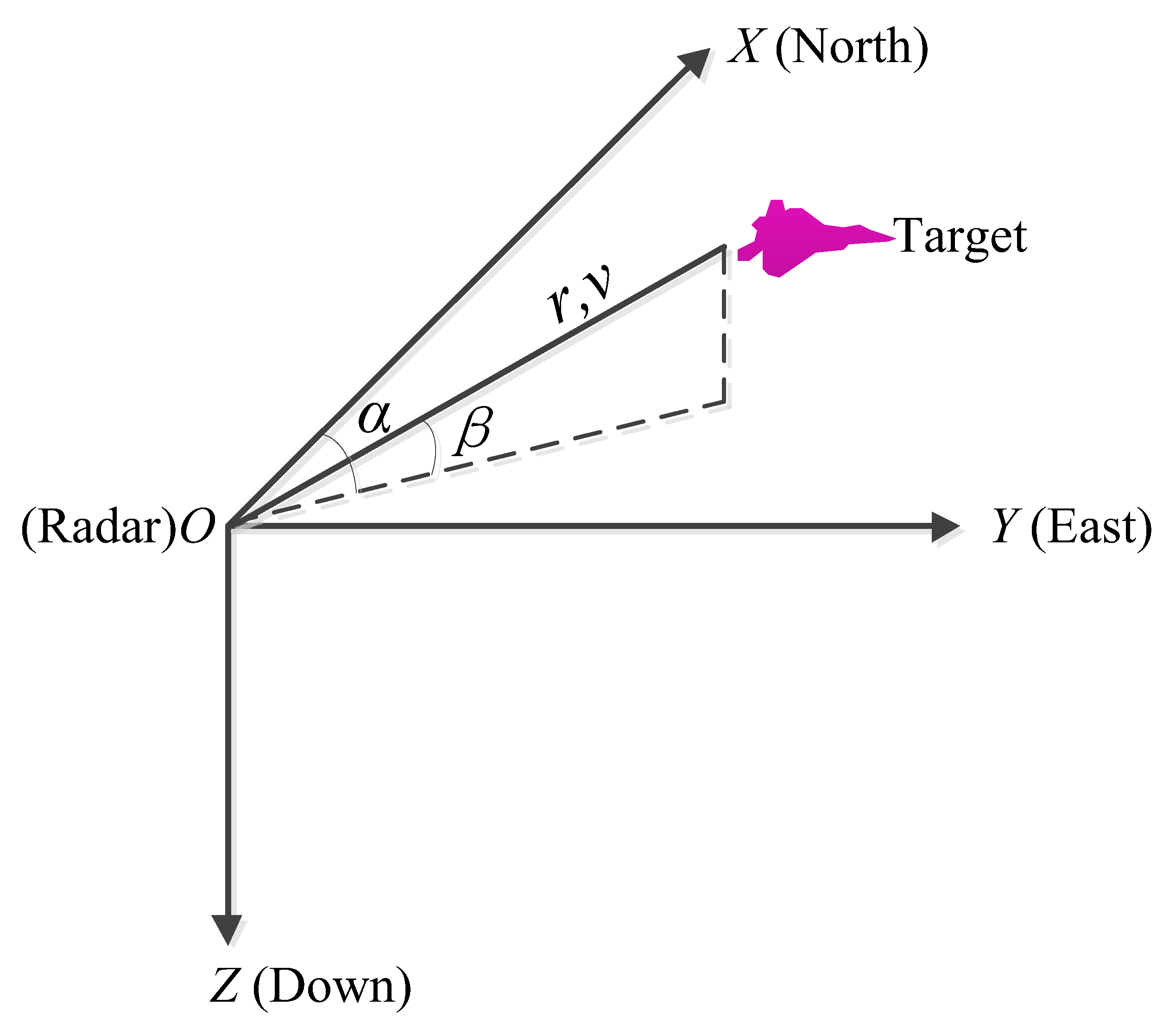
Based on the detection principle of radar, the geometric relationship of the target and radar is shown in Figure 1. The measurement of the radar consists of radial distance, radial velocity, azimuth, and elevation. The measurement equation is formulated as
z k + 1 = r α β v + v k + 1 = h ( x k + 1 , x k + 1 r ) + v k + 1 = ( x k + 1 t x k + 1 r ) 2 + ( y k + 1 t y k + 1 r ) 2 + ( z k + 1 t z k + 1 r ) 2 arctan ( y k + 1 t y k + 1 r x k + 1 t x k + 1 r ) arcsin ( z k + 1 t z k + 1 r ( x k + 1 t x k + 1 r ) 2 + ( y k + 1 t y k + 1 r ) 2 + ( z k + 1 t z k + 1 r ) 2 ) ( ( x k + 1 t x k + 1 r ) ( x ˙ k + 1 t x ˙ k + 1 r ) + ( y k + 1 t y k + 1 r ) ( y ˙ k + 1 t y ˙ k + 1 r ) + ( z k + 1 t z k + 1 r ) ( z ˙ k + 1 t z ˙ k + 1 r ) ) ( x k + 1 t x k + 1 r ) 2 + ( y k + 1 t y k + 1 r ) 2 + ( z k + 1 t z k + 1 r ) 2 + v k + 1
x k + 1 r = [ x k + 1 r , x ˙ k + 1 r , x ¨ k + 1 r , y k + 1 r , y ˙ k + 1 r , y ¨ k + 1 r , z k + 1 r , z ˙ k + 1 r , z ¨ k + 1 r ] T
where x k + 1 r is the state of the radar at time k+1. ( x k + 1 r , y k + 1 r , z k + 1 r ) and ( x ˙ k + 1 r , y ˙ k + 1 r , z ˙ k + 1 r ) are the position and velocity of the radar in the North-East-Down coordinate system, respectively. v k + 1 is the measurement noise of the radar, and R k + 1 4 × 4 is defined as its nominal covariance matrix. The state of the radar can be obtained through the navigation information. Based on this measurement equation, the Gaussian kernel function G 2 from the sub-model state update step is changed as
G 2 = G σ ( z k + 1 h ( x k + 1 ) , R k + 1 )
According to Equation (53), Equation (24) is changed as
( aG 1 + ( 1 a ) G 2 ) / x k + 1 = aG 1 ( P k + 1 k i ) 1 ( x k + 1 x k + 1 k i ) / σ 2 ( 1 a ) G 2 ( h ( x k + 1 ) x k + 1 ) T ( R k + 1 ) 1 ( z k + 1 h ( x k + 1 ) ) / σ 2  
Let ( aG 1 + ( 1 a ) G 2 ) / x k + 1 = 0 , then we have
aG 1 ( P k + 1 k i ) 1 x k + 1 = aG 1 ( P k + 1 k i ) 1 x k + 1 k i + ( 1 a ) G 2 ( h ( x k + 1 ) x k + 1 ) T ( R k + 1 ) 1 ( z k + 1 h ( x k + 1 ) )
Based on the Taylor’s first-order expansion formula, h ( x k + 1 ) can be approximated as
h ( x k + 1 ) h ( x k + 1 k i ) + H k + 1 k i ( x k + 1 x k + 1 k i )
H k + 1 k i = h ( x k + 1 ) x k + 1 x k + 1 = x k + 1 k i
According to Equations (55)–(57), x k + 1 is formulated as
( aG 1 ( P k + 1 k i ) 1 + ( 1 a ) G 2 ( H k + 1 k i ) T ( R k + 1 ) 1 H k + 1 k i ) ( x k + 1 x k + 1 k i ) = ( 1 a ) G 2 ( H k + 1 k i ) T ( R k + 1 ) 1 ( z k + 1 h ( x k + 1 k i ) ) x k + 1 = x k + 1 k i + ( aG 1 ( P k + 1 k i ) 1 + ( 1 a ) G 2 ( H k + 1 k i ) T ( R k + 1 ) 1 H k + 1 k i ) 1             × ( 1 a ) G 2 ( H k + 1 k i ) T ( R k + 1 ) 1 ( z k + 1 h ( x k + 1 k i ) )
According to Equations (25) and (58), it can be found that the update state of i-th sub-model from a radar system can be obtained by using H k + 1 k i and h ( x k + 1 k i ) to replace H k + 1 i and x k + 1 k i in Equations (26) and (27). Based on this, x k + 1 k + 1 i is formulated as
x k + 1 k + 1 i = x k + 1 k i + K k + 1 k i ( z k + 1 h ( x k + 1 k i ) )
K k + 1 k i = P k + 1 k i ( H k + 1 k i ) T ( ( H k + 1 k i P k + 1 k i ( H k + 1 k i ) T + ( a R k + 1 i / ( G 3 ( 1 a ) ) ) ) 1
G 3 = G σ ( z k + 1 h ( x k + 1 k i ) , R k + 1 )
According to Equation (59), x ˜ k + 1 i is formulated as
x ˜ k + 1 i = x k + 1 x k + 1 k + 1 i = ( x k + 1 x k + 1 k i ) K k + 1 k i ( h ( x k + 1 ) h ( x k + 1 k i ) ) K k + 1 k i v k + 1 i ( x k + 1 x k + 1 k i ) K k + 1 k i H k + 1 k i ( x k + 1 x k + 1 k i ) K k + 1 k i v k + 1 i = ( I K k + 1 i H k + 1 k i ) ( x k + 1 x k + 1 k i ) K k + 1 k i v k + 1 i
Similarly, the measurement noise covariance of a sub-model is modified as a R k + 1 / ( G 3 ( 1 a ) ) , and the estimation error covariance P k + 1 k + 1 i is formulated as
P k + 1 k + 1 i = ( I K k + 1 i H k + 1 k i ) P k + 1 k i
In the model probability update step, the innovation error Δ z k + 1 i and covariance S k + 1 i is formulated as
Δ z k + 1 i = z k + 1 H k + 1 k i x k + 1 k i
S k + 1 i = H k + 1 k i P k + 1 k ( H k + 1 k i ) T + a R k + 1 / ( G 3 ( 1 a ) )
Finally, the fusion state x k + 1 k + 1 and covariance P k + 1 k + 1 can be calculated by using Equations (35), (36), and (41). In summary, the pseudo-code of the WMCC-IMM filter in a radar system is summarized in Algorithm 2.
Algorithm 2: The pseudo-code of the WMCC-IMM filter in a radar system
for k = 0:L − 1
Input:  x k k ,   P k k ,   F k i ,   Q k i ,   z k + 1 ,   R k + 1 i ,   a
Using Equations (4) and (5) to calculate P k k i , 0
Using Equation (22) to calculate x k + 1 k i   and   P k + 1 k i
Using Equation (57) to calculate H k + 1 k i
Using Equations (60) and (61) to calculate K k + 1 k i
Using Equations (59) and (63) x k + 1 k + 1 i   and   P k + 1 k + 1 i
Using Equations (64), (65), (13), and (14) (13), (14), (64) and (65) to calculate μ k + 1 k + 1 i
Using Equations (35), (36), and (41) to calculate x k + 1 k + 1   and P k + 1 k + 1
Output:   x k + 1 k + 1 ,   P k + 1 k + 1
end

4. Experimental Results

4.1. Case 1. Maneuvering Target Tracking Simulation Experiment

In this section, a maneuvering target tracking example [27] is used to verify the effectiveness of the proposed filter. The target moves in a two-dimensional plane, and the target state consists of position and velocity. The number of sub-models is 2. The state transition equation of each sub-model is a constant turn (CT) model [27], and the measurement consists of the position information. The turning rate w 1 and w 2 are set as π / 40 rad / s and π / 40 rad / s , respectively. The initial true state x 0 and covariance P 0 0 i ( i = 1 , 2 ) are set as [100 m, 5 m/s, 100 m, 5 m/s] and diag([100 m2, 25 m2/s2, 100 m2, 25 m2/s2]), respectively. The actual motion of the target follows the CT model. For 1–50 s, the turning rate is w 1 . For 51–100 s, the turning rate is w 2 . The initial state x 0 0 i ( i = 1 , 2 ) of each sub-model is chosen from N ( x 0 0 i ; x 0 , P 0 0 i ) . The total time L is 100 s, and the number of Monte Carlo runs is 100. The Markov transition matrix π is set as 0.95 0.05 0.05 0.95 . The initial weight of each sub-model is 0.5. The process noise follows the Gaussian distribution, while the measurement noise follows the Gaussian mixture distribution [12]. At this time, w k + 1 i and v k + 1 i ( i = 1 , 2 ) are formulated as
w k i N ( w k i ; 0 , Q k i )
v k + 1 i 0.9 N ( v k + 1 i ; 0 , R k + 1 i ) + 0.1 N ( v k + 1 i ; 0 , 100 R k + 1 i )
The process noise covariance matrix Q k i ( i = 1 , 2 ) and measurement noise covariance matrix R k + 1 i ( i = 1 , 2 ) are set as
Q k i = q 1 / 3 1 / 2 0 0 1 / 2 1 0 0 0 0 1 / 3 1 / 2 0 0 1 / 2 1
R k + 1 i = 100 m 2 0 0 100 m 2
where q = 1   m 2 / s 3 . The root mean square error (RMSE) and the time-averaged RMSE (TRMSE) are used as performance evaluating criteria. The IMM [9], IMM-VB [12], and IMM-MCC [21] filters are used to compare with the WMCC-IMM filter. For a fair comparison, the kernel function from the IMM-MCC filter is the same as that from the WMCC-IMM filter, and the kernel bandwidths from the IMM-MCC and WMCC-IMM filters are set as 5. The degree of freedom parameter and iteration times from the IMM-VB filter [12] are set as 1 and 3, respectively.
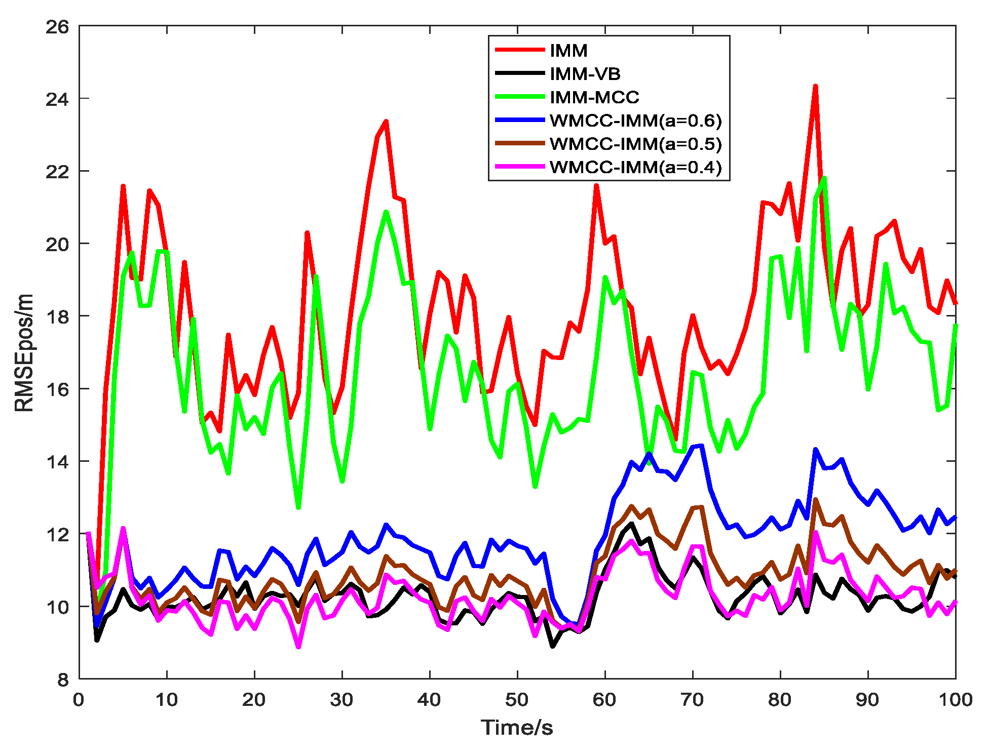
Figure 2 and Figure 3 and Table 1 show the computational time in the one-step state update process and the RMSEs and TRMSEs of position and velocity from the IMM, IMM-VB, IMM-MCC, and WMCC-IMM filters. It can be found that the computational time of the WMCC-IMM filter is close to that of the IMM and IMM-MCC filters, and the IMM-VB filter has the highest computational complexity among these four filters. The estimation performance of the IMM filter is the worst, and the IMM-VB filter has the best state estimation performance. When a is set to a value slightly smaller than 0.5, the WMCC-IMM filter has better state estimation performance. When a = 0.5 , the WMCC-IMM filter becomes the MCC-IMM filter, which means that simplifying the state interaction and using the MCC to realize the state fusion is an effective way to improve the state estimation performance. In addition, under the condition of this parameter setting, the IMM-VB filter improves the estimation accuracy of position and velocity by 5.6% and 6%, respectively, compared with the WMCC-IMM filter, but its computational time is increased by 19.2%. Therefore, it can be considered that when the hardware has limited computational performance, the WMCC-IMM filter is a better choice for state estimation of the multiple-model system under outlier interference.
To test the effect of kernel bandwidth for the IMM-MCC and WMCC-IMM filters, Table 2 shows the TRMSEs of position and velocity from these two filters under different kernel bandwidths. It can be found that when the kernel bandwidth is too small, the IMM-MCC filter will be singular, resulting in its failure to work, while the WMCC-IMM filter can be used normally. With the increase of kernel bandwidth, the WMCC-IMM filter still has better state estimation performance than the IMM-MCC filter [26].

4.2. Case 2. Maneuvering Target Tracking Actual Test Experiment

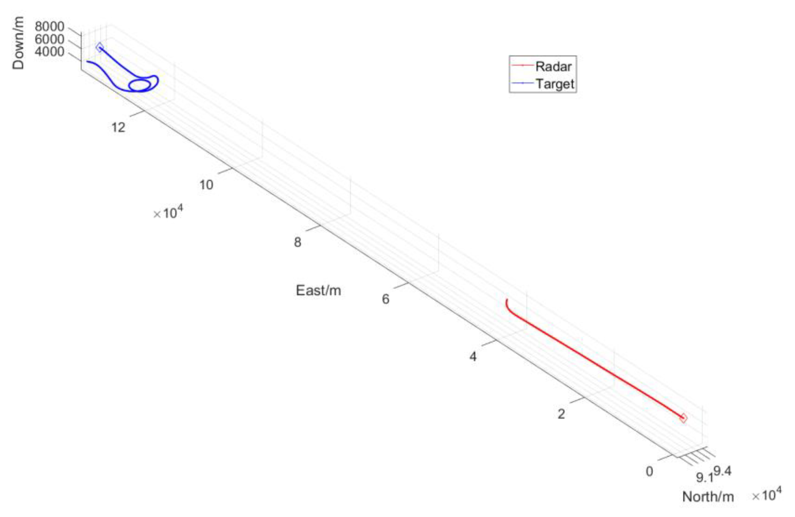
In case 2, a set of maneuvering target tracking actual test data is used to test the state estimation performance of different filters. The relative situation of radar and target is shown in Figure 4.
The motion model set consists of the CV model, the constant acceleration (CA) model, and the current statistics (CS) model [28]. The Markov transition matrix π is set as 0.8 0.1 0.1 0.1 0.8 0.1 0.1 0.1 0.8 . Since the true state of the target cannot be obtained in the actual target tracking process, the initial state of each sub-model is set by using the initial measurement, and it can be calculated as
x 0 t = r 0 c o s β 0 c o s α 0 + x 0 r x ˙ 0 t = v 0 c o s β 0 c o s α 0 + x ˙ 0 r x ¨ 0 t = 0 y 0 t = r 0 c o s β 0 s i n α 0 + y 0 r y ˙ 0 t = v 0 c o s β 0 s i n α 0 + y ˙ 0 r y ¨ 0 t = 0 z 0 t = r 0 s i n β 0 + z 0 r z ˙ 0 t = v 0 s i n β 0 + z ˙ 0 r z ¨ 0 t = 0
The initial covariance P 0 0 i ( i = 1 , 2 , 3 ) of each sub-model is set as
P 0 0 i = d i a g 640000 m 2 , 800 m 2 / s 2 , 0 , 640000 m 2 , 800 m 2 / s 2 , 0 , 640000 m 2 , 800 m 2 / s 2 , 0
The initial weight of each sub-model is 0.33. The process noise covariance matrix Q k , CV , Q k , CA , Q k , CS and measurement noise covariance matrix R k + 1 are set as
Q k , CV = 0.25 T 4 0.5 T 3 0 0 0 0 0 0 0 0.5 T 3 T 2 0 0 0 0 0 0 0 0 0 0 0 0 0 0 0 0 0 0 0 0.25 T 4 0.5 T 3 0 0 0 0 0 0 0 0.5 T 3 T 2 0 0 0 0 0 0 0 0 0 0 0 0 0 0 0 0 0 0 0 0.25 T 4 0.5 T 3 0 0 0 0 0 0 0 0.5 T 3 T 2 0 0 0 0 0 0 0 0 0 0
Q k , CA = 0.05 T 5 0.125 T 4 0.167 T 3 0 0 0 0 0 0 0.125 T 4 0.33 T 3 0.5 T 2 0 0 0 0 0 0 0.167 T 3 0.5 T 2 T 0 0 0 0 0 0 0 0 0 0.05 T 5 0.125 T 4 0.167 T 3 0 0 0 0 0 0 0.125 T 4 0.33 T 3 0.5 T 2 0 0 0 0 0 0 0.167 T 3 0.5 T 2 T 0 0 0 0 0 0 0 0 0 0.05 T 5 0.125 T 4 0.167 T 3 0 0 0 0 0 0 0.125 T 4 0.33 T 3 0.5 T 2 0 0 0 0 0 0 0.167 T 3 0.5 T 2 T
Q k , CS = q 11 q 12 q 13 0 0 0 0 0 0 q 12 q 22 q 23 0 0 0 0 0 0 q 13 q 23 q 33 0 0 0 0 0 0 0 0 0 q 11 q 12 q 13 0 0 0 0 0 0 q 12 q 22 q 23 0 0 0 0 0 0 q 13 q 23 q 33 0 0 0 0 0 0 0 0 0 q 11 q 12 q 13 0 0 0 0 0 0 q 12 q 22 q 23 0 0 0 0 0 0 q 13 q 23 q 33
R k + 1 = 6400 m 2 0 0 0 0 6.85 × 10 6 ( rad 2 ) 0 0 0 0 6.85 × 10 6 ( rad 2 ) 0 0 0 0 4 m 2 / s 2
where
q 11 = 1 4 b T e b T e 2 b T 2 + 2 b T 2 b 2 T 2 + 2 b 3 T 3 3 2 b 5 q 12 = 1 + ( 2 b T 2 ) e b T + e 2 b T 2 2 b T + b 2 T 2 2 b 4 q 13 = 1 2 e b T + e 2 b T 2 2 b 3 q 22 = 3 + 2 b T + 4 e b T e 2 b T 2 2 b 3 q 23 = 1 2 e b T + e 2 b T 2 2 b 2 q 23 = 1 + e 2 b T 2 2 b b = 0.1
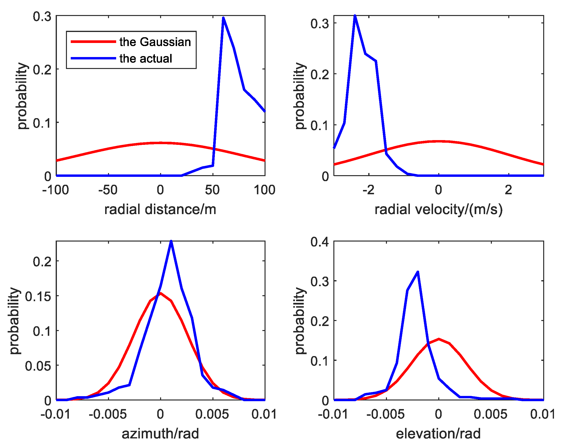
Based on the measurement noise covariance, the probability distribution of Gaussian measurement noise and actual noise is shown in Figure 5. It can be seen that the actual noise does not follow the Gaussian distribution. The measurements of radial distance and radial velocity have more outliers.
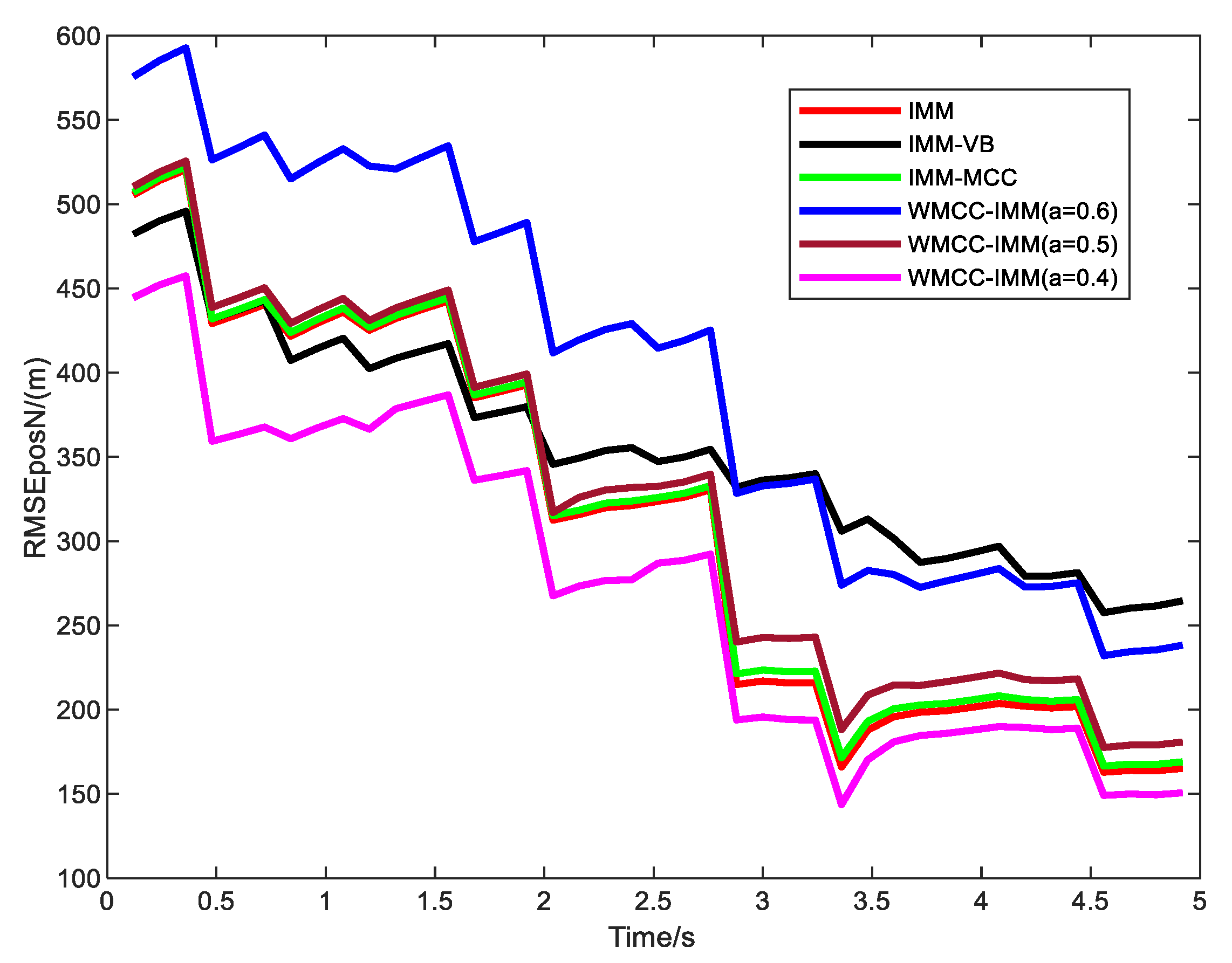
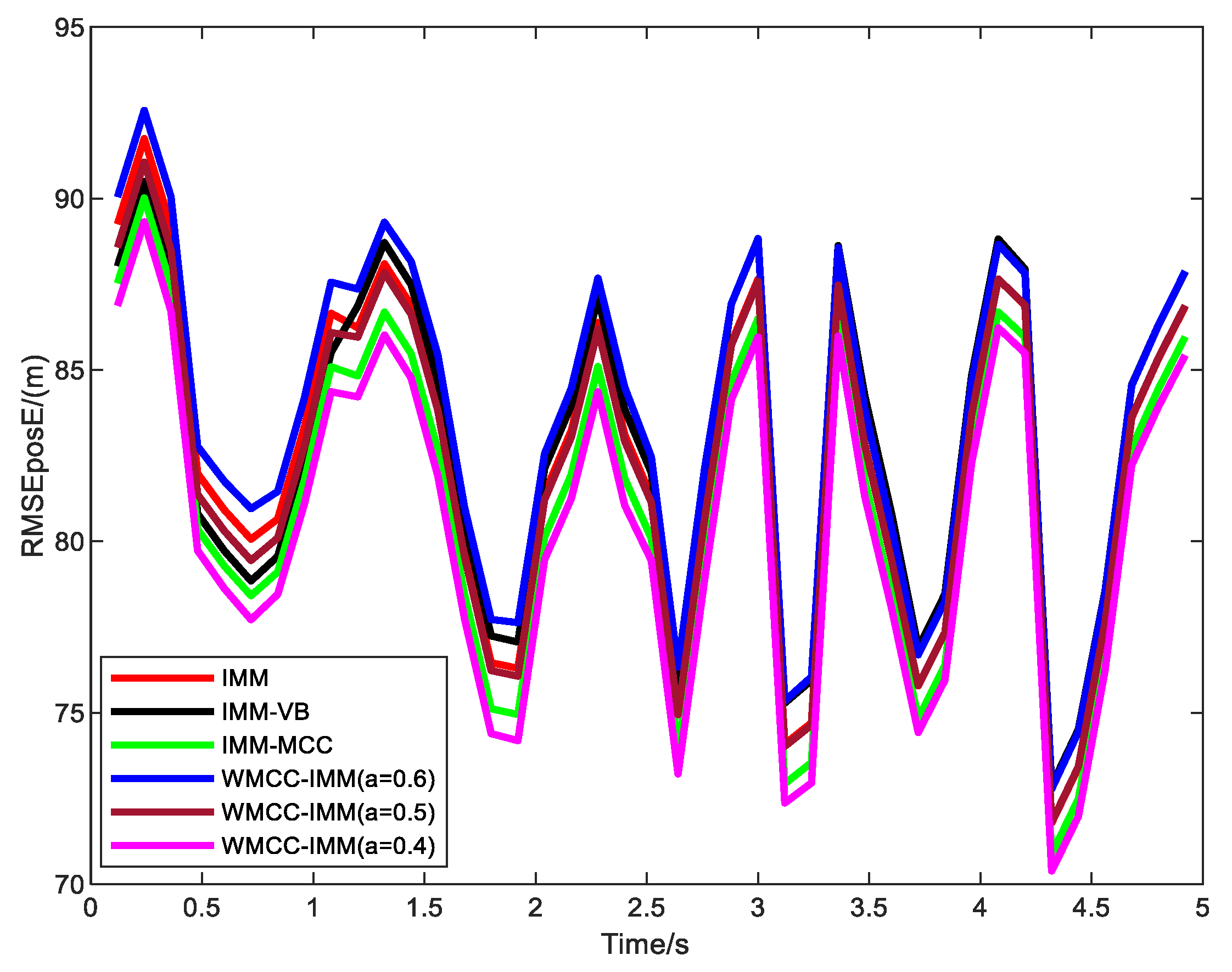
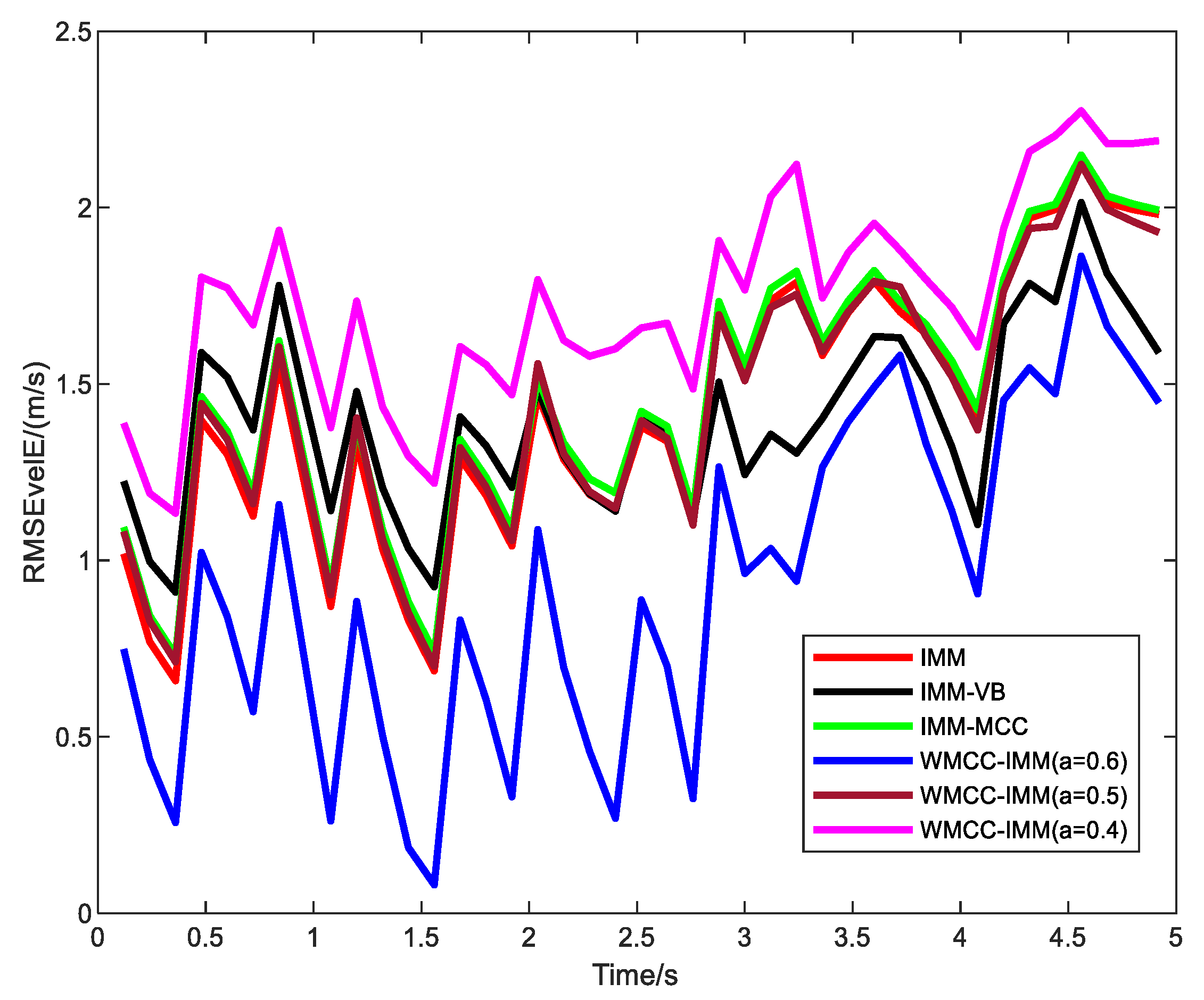
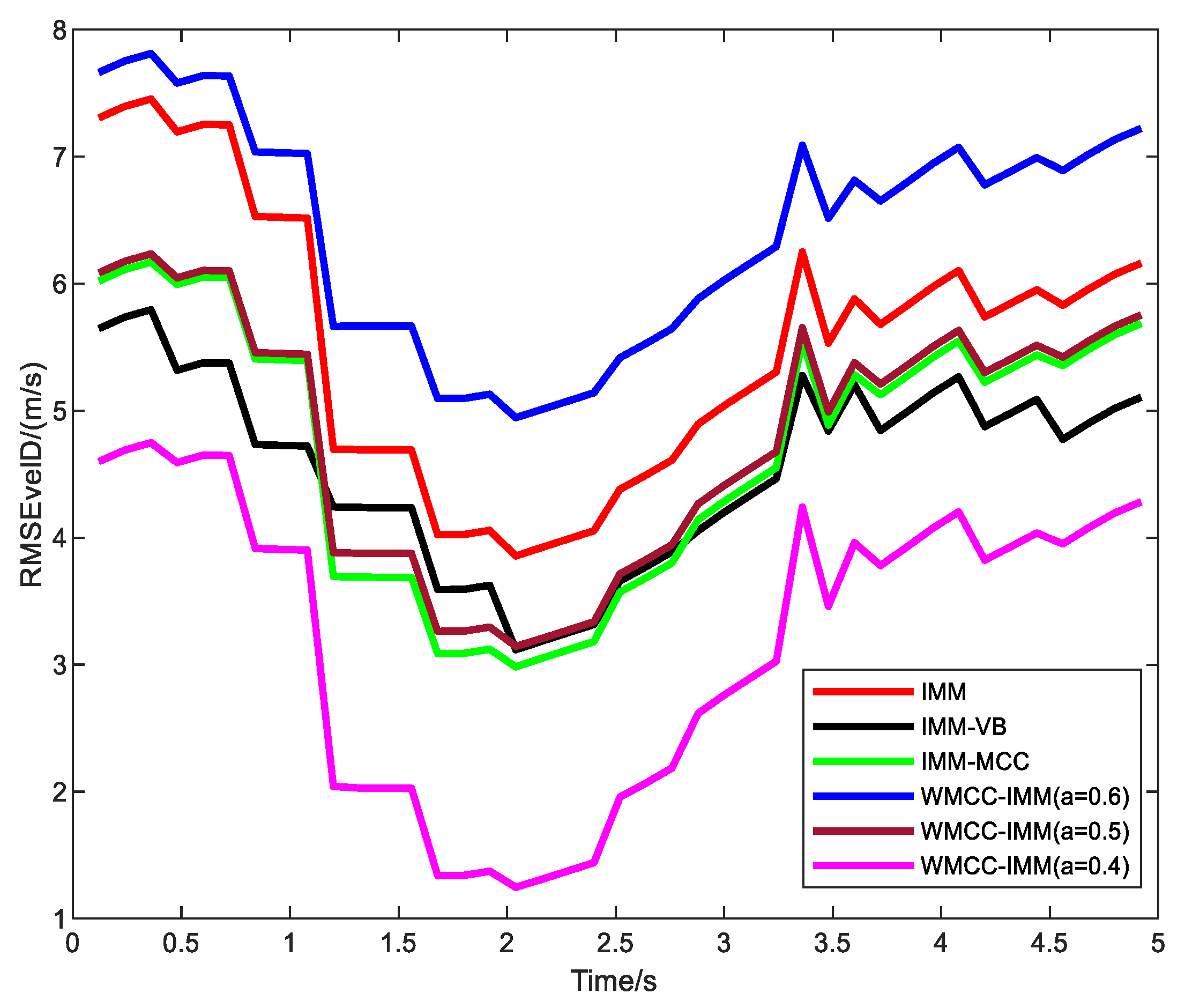
During the process of actual maneuvering target tracking to assist the subsequent guidance mission, the estimation performance of each dimension from state is given more attention rather than the overall estimation performance of state, and the combat platform has stringent requirements for the estimation accuracy of position and velocity. Because of this, the estimation accuracy of different filters in position and velocity is compared. The RMSEs of position and velocity in the North-East-Down coordinate system from different filters are shown in Figure 6, Figure 7, Figure 8, Figure 9, Figure 10 and Figure 11, and the corresponding TRMSEs are shown in Table 3. It can be seen that when a = 0.4 , the WMCC-IMM filter exhibits the best estimation performance in terms of north position, north velocity, east position and down velocity. On the other hand, the IMM-VB filter demonstrates the best estimation performance in terms of down position and east velocity. Based on the RMSEs of position and velocity in the North-East-Down coordinate system from different filters, when a = 0.4 , the computed results of the RMSEs of position and velocity from the WMCC-IMM filter are 343.85 m and 21.11 m/s, respectively. The computed results of the RMSEs of position and velocity from the IMM-VB filter are 385.06 m and 30.68 m/s, respectively. Therefore, the WMCC-IMM filter has better estimation performance than the IMM-VB filter.
In addition to position and velocity, the entry angle [29] is another crucial parameter of interest for the combat platform because the entry angle can be used to discern the threat level of the target. The estimation error of entry angle Δ e a k is formulated as
Δ e a k = arctan ( y ˙ ¯ k t y ˙ ¯ k r x ˙ ¯ k t x ˙ ¯ k r ) + α ¯ k arctan ( y ˙ k | k t y ˙ ¯ k r x ˙ k | k t x ˙ ¯ k r ) α k
where x ˙ ¯ k t and y ˙ ¯ k t are the true north velocity and east velocity of the target at time k, respectively. x ˙ ¯ k r and y ˙ ¯ k r are the true north velocity and east velocity of the radar at time k, respectively. α ¯ k is the true azimuth at time k. It can be seen that estimation error of entry angle is influenced by the estimation errors of azimuth, target’s north velocity, and target’s east velocity. Using Δ e a k , the RMSE of entry angle can be obtained.
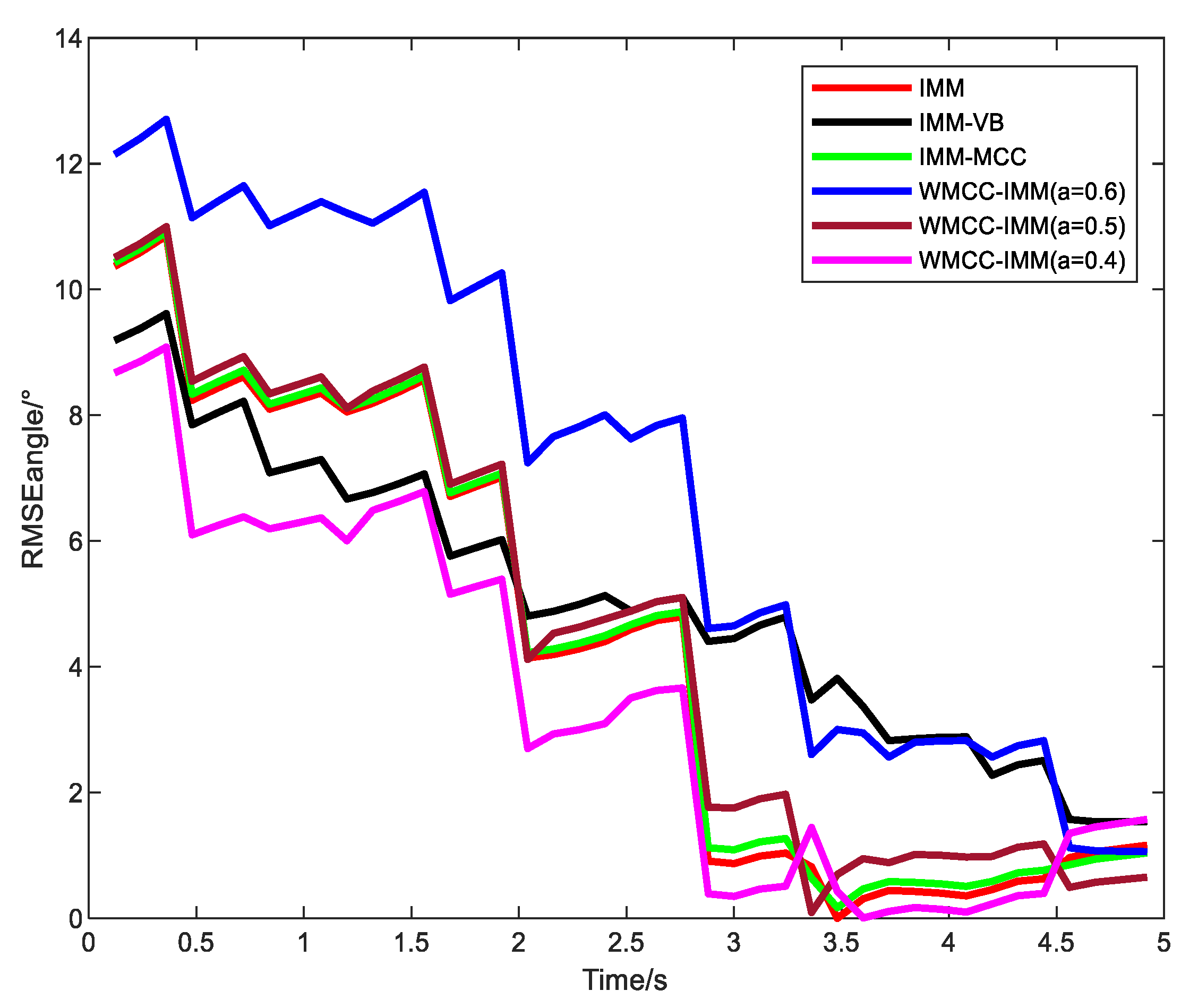
To further compare the estimation performance of different filters, the estimation accuracy of entry angle from different filters is tested. Figure 12 shows the RMSEs of entry angle from different filters, and Table 4 shows the TRMSEs of entry angle from different filters. Since the estimation error of east velocity from different filters is small and the estimation error of north velocity from different filters is large, the filter that has the best estimation performance of north velocity tends to exhibit superior performance in entry angle estimation. Therefore, the WMCC-IMM filter, wherein a is set as 0.4, has better estimation performance of entry angle than other filters. In conclusion, when a = 0.4 , the WMCC-IMM filter has better state estimation performance than the IMM, IMM-VB, and IMM-MCC filters under non-Gaussian measurement noise.

5. Conclusions

In this article, a novel WMCC-based IMM filter is proposed to solve the state estimation problem in maneuvering target tracking under outlier interference. Different from the IMM-VB and IMM-MCC filters, the WMCC-IMM filter uses the previous fusion state to simplify the state interaction step and adopts the WMCC to realize the state estimation and fusion steps. The specific steps of the WMCC-IMM filter in a radar system are also outlined. The experimental test results show that the WMCC-IMM filter has better state estimation performance than the IMM, IMM-VB, and IMM-MCC filters under outlier interference. The accuracy of the target motion model greatly affects the estimation performance of the proposed filter. Therefore, in future work, we need to further study the modeling of the target motion characteristics to improve the estimation performance of the proposed filter for high-maneuvering targets, such as a hypersonic vehicle.

Author Contributions

Conceptualization, L.H. and B.L.; methodology, L.H. and P.Y.; software, L.H.; validation, L.H., P.Y. and J.W.; formal analysis, L.H. and P.Y.; writing—original draft preparation, L.H.; writing—review and editing, B.L., P.Y. and C.S.; funding acquisition, B.L. and P.Y. All authors have read and agreed to the published version of the manuscript.

Funding

This research was funded in part by the Fundamental Research Funds for the Central Universities under grant number G2022KY0602, in part by the Technology on Electromagnetic Space Operations and Applications Laboratory under grant number 2022ZX0090, in part by the key core technology research plan of Xi’an under grant number 21RGZN0016, in part by the National Nature Science Foundation of China under grant number 62003267, and in part by the Jiangsu Funding Program for Excellent Postdoctoral Talent under grant number 2023ZB624.

Data Availability Statement

Data sharing not applicable. The simulation data for case 1 can be obtained based on simulation conditions. Due to restrictions eg privacy, the case 2’s data is not suitable for sharing.

Conflicts of Interest

The authors declare no conflict of interest.

Appendix A. The Derivation of K k + 1 i

In the derivation process of K k + 1 i , the matrix inversion formula needs to be used. The matrix inversion formula is formulated as
( A + U C V ) 1 = A 1 U ( C 1 + V A 1 U ) 1 V A 1
Using Equation (A1), K k + 1 i is formulated as
K k + 1 i = ( ( P k + 1 k i ) 1 + ( H k + 1 i ) T ( a R k + 1 i / ( G 3 ( 1 a ) ) ) 1 H k + 1 i ) 1 ( H k + 1 i ) T ( a R k + 1 i / ( G 3 ( 1 a ) ) ) 1 = ( P k + 1 k i P k + 1 k i ( H k + 1 i ) T ( ( a R k + 1 i / ( G 3 ( 1 a ) ) ) + H k + 1 i P k + 1 k i ( H k + 1 i ) T ) 1 H k + 1 i P k + 1 k i ) ( H k + 1 i ) T ( a R k + 1 i / ( G 3 ( 1 a ) ) ) 1 = P k + 1 k i ( H k + 1 i ) T ( a R k + 1 i / ( G 3 ( 1 a ) ) ) 1 P k + 1 k i ( H k + 1 i ) T ( ( a R k + 1 i / ( G 3 ( 1 a ) ) ) + H k + 1 i P k + 1 k i ( H k + 1 i ) T ) 1 H k + 1 i P k + 1 k i ( H k + 1 i ) T ( a R k + 1 i / ( G 3 ( 1 a ) ) ) 1 = P k + 1 k i ( H k + 1 i ) T ( ( a R k + 1 i / ( G 3 ( 1 a ) ) ) 1 ( ( a R k + 1 i / ( G 3 ( 1 a ) ) ) + H k + 1 i P k + 1 k i ( H k + 1 i ) T ) 1 H k + 1 i P k + 1 k i ( H k + 1 i ) T ( a R k + 1 i / ( G 3 ( 1 a ) ) ) 1 ) = P k + 1 k i ( H k + 1 i ) T ( ( ( a R k + 1 i / ( G 3 ( 1 a ) ) ) + H k + 1 i P k + 1 k i ( H k + 1 i ) T ) 1 ( a R k + 1 i / ( G 3 ( 1 a ) ) ) ( a R k + 1 i / ( G 3 ( 1 a ) ) ) 1 ) = P k + 1 k i ( H k + 1 i ) T ( ( ( a R k + 1 i / ( G 3 ( 1 a ) ) ) + H k + 1 i P k + 1 k i ( H k + 1 i ) T ) 1

References

  1. Wu, P.L.; Li, X.X.; Zhang, L.Z. Tracking algorithm with radar and IR sensors using a novel adaptive grid interacting multiple model. IET Sci. Meas. Technol. 2014, 8, 270–276. [Google Scholar] [CrossRef]
  2. Gustafsson, F.; Gunnarsson, F. Particle filters for positioning, navigation, and tracking. IEEE Trans. Signal Process. 2002, 50, 425–437. [Google Scholar] [CrossRef]
  3. Jordi, V.V.; Damien, V. Recursive linearly constrained Wiener filter for robust multi-channel signal processing. Signal Process. 2020, 167, 107291. [Google Scholar]
  4. Blair, W.D.; Bar-Shalom, Y. MSE Design of Nearly Constant Velocity Kalman Filters for Tracking Targets with Deterministic Maneuvers. IEEE Trans. Aerosp. Electron. Syst. 2023, 59, 4180–4191. [Google Scholar] [CrossRef]
  5. Montañez, O.J.; Suarez, M.J.; Fernandez, E.A. Application of Data Sensor Fusion Using Extended Kalman Filter Algorithm for Identification and Tracking of Moving Targets from LiDAR-Radar Data. Remote Sens. 2023, 15, 3396. [Google Scholar] [CrossRef]
  6. Kalman, R.E. A New Approach to Linear Filtering and Prediction Problems. J. Basic Eng. 1960, 82, 35–45. [Google Scholar] [CrossRef]
  7. Wang, J.L.; Wang, J.H.; Zhang, D. Kalman Filtering through the Feedback Adaption of Prior Error Covariance. Signal Process. 2018, 152, 47–53. [Google Scholar] [CrossRef]
  8. Liu, Y.; Ning, X.; Li, J. Adaptive Central Difference Kalman Filter with Unknown Measurement Noise Covariance and Its Application to Airborne POS. IEEE Sens. J. 2021, 21, 9927–9936. [Google Scholar] [CrossRef]
  9. Mazor, E.; Averbuch, A.; Bar-Shalom, Y. Interacting multiple model methods in target tracking: A survey. IEEE Trans. Aerosp. Electron. Syst. 1998, 34, 103–123. [Google Scholar] [CrossRef]
  10. Qu, H.Q.; Pang, L.P.; Li, S.H. A novel interacting multiple model algorithm. Signal Process. 2009, 89, 2171–2177. [Google Scholar] [CrossRef]
  11. Ruan, Y.; Hong, L. Use of the interacting multiple model algorithm with multiple sensors. Math. Comput. Model. 2006, 44, 332–341. [Google Scholar] [CrossRef]
  12. Yun, P.; Wu, P.L.; He, S. An IMM-VB Algorithm for Hypersonic Vehicle Tracking with Heavy Tailed Measurement Noise. In Proceedings of the 2018 International Conference on Control, Automation and Information Sciences (ICCAIS), Hangzhou, China, 24–27 October 2018; pp. 169–174. [Google Scholar]
  13. Yun, P.; Wu, P.L.; He, S. Pearson type VII distribution-based robust Kalman filter under outliers interference. IET Radar Sonar Navig. 2019, 13, 1389–1399. [Google Scholar]
  14. Yun, P.; Wu, P.L.; He, S. Robust Kalman Filter with Fading Factor under State Transition Model Mismatch and Outliers Interference. Circuits Syst. Signal Process. 2021, 40, 2443–2463. [Google Scholar] [CrossRef]
  15. Chen, B.D.; Xing, L.; Liang, J. Steady-state mean square error analysis for adaptive filtering under the maximum correntropy criterion. IEEE Signal Process. Lett. 2014, 21, 880–884. [Google Scholar]
  16. Chen, B.D.; Liu, X.; Zhao, H.Q. Maximum correntropy Kalman filter. Automatica 2017, 76, 70–77. [Google Scholar] [CrossRef]
  17. He, J.J.; Sun, C.K.; Zhang, B.S. Maximum Correntropy Square-Root Cubature Kalman Filter for Non-Gaussian Measurement Noise. IEEE Access 2020, 8, 70162–70170. [Google Scholar] [CrossRef]
  18. Liu, X.; Qu, H.; Zhao, J. Maximum Correntropy Unscented Kalman Filter for Spacecraft Relative State Estimation. Sensors 2016, 16, 1530. [Google Scholar] [CrossRef] [PubMed]
  19. Li, S.X.; Xu, B.; Wang, L.Z. Improved Maximum Correntropy Cubature Kalman Filter for Cooperative Localization. IEEE Sens. J. 2020, 20, 13585–13595. [Google Scholar] [CrossRef]
  20. Wang, G.; Li, N.; Zhang, Y. Maximum correntropy unscented Kalman and information filters for non-Gaussian measurement noise. J. Frankl. Inst. 2017, 354, 8659–8677. [Google Scholar] [CrossRef]
  21. Wang, G.; Xue, R.; Wang, J.X. A distributed maximum correntropy Kalman filter. Signal Process. 2019, 160, 247–251. [Google Scholar] [CrossRef]
  22. Wang, G.Q.; Zhang, Y.G.; Wang, X.D. Maximum Correntropy Rauch-Tung-Striebel Smoother for Nonlinear and Non Gaussian Systems. IEEE Trans. Autom. Control 2021, 66, 1270–1277. [Google Scholar] [CrossRef]
  23. Bao, Z.C.; Jiang, Q.X.; Liu, F.Z. Multiple model efficient particle filter based track-before-detect for maneuvering weak targets. J. Syst. Eng. Electron. 2020, 31, 647–656. [Google Scholar]
  24. Ebrahimi, M.; Ardeshiri, M.; Khanghah, S.A. Bearing-only 2D maneuvering target tracking using smart interacting multiple model filter. Digit. Signal Process. 2022, 126, 103497. [Google Scholar] [CrossRef]
  25. Yang, B.; Zhu, S.Q.; He, X.P. IMM Robust Cardinality Balance Multi-Bernoulli Filter for Multiple Maneuvering Target Tracking with Interval Measurement. Chin. J. Electron. 2021, 30, 1141–1151. [Google Scholar]
  26. Fan, X.X.; Wang, G.; Han, J.C. Interacting Multiple Model Based on Maximum Correntropy Kalman Filter. IEEE Trans. Circuits Syst. II Express Briefs 2021, 68, 3017–3021. [Google Scholar] [CrossRef]
  27. Yun, P.; Wu, P.L.; Li, X.X. Variational Bayesian Probabilistic Data Association Algorithm. Acta Autom. Sin. 2022, 48, 2486–2495. [Google Scholar] [CrossRef]
  28. Yi, S.; Jin, X.; Su, T. An improved online denoising algorithm based on Kalman filter and adaptive current statistics model. In Proceedings of the 2017 9th International Conference on Modelling, Identification and Control (ICMIC), Kunming, China, 10–12 July 2017; pp. 782–786. [Google Scholar]
  29. Guo, Q.; He, S.; Cheng, J. A Threat Evaluation Method of Autonomous UAV Avoidance Missile. Aeronaut. Sci. Technol. 2022, 33, 8–14. [Google Scholar]
Figure 1. The geometric relationship of the target and radar.
Remotesensing 15 04513 g001
Figure 2. The RMSEs of position from different filters in case 1.
Remotesensing 15 04513 g002
Figure 3. The RMSEs of velocity from different filters in case 1.
Remotesensing 15 04513 g003
Figure 4. The relative situation of radar and target in case 2.
Remotesensing 15 04513 g004
Figure 5. The probability distribution of Gaussian measurement noise and actual noise in case 2.
Remotesensing 15 04513 g005
Figure 6. The RMSEs of north position from different filters in case 2.
Remotesensing 15 04513 g006
Figure 7. The RMSEs of east position from different filters in case 2.
Remotesensing 15 04513 g007
Figure 8. The RMSEs of down position from different filters in case 2.
Remotesensing 15 04513 g008
Figure 9. The RMSEs of north velocity from different filters in case 2.
Remotesensing 15 04513 g009
Figure 10. The RMSEs of east velocity from different filters in case 2.
Remotesensing 15 04513 g010
Figure 11. The RMSEs of down velocity from different filters in case 2.
Remotesensing 15 04513 g011
Figure 12. The RMSEs of entry angle from different filters in case 2.
Remotesensing 15 04513 g012
Table 1. The computational time in the one-step state update process and the TRMSEs from different filters.
FiltersPos/mVel/(m/s)Time/ms
IMM18.195.260.308
IMM-VB10.283.740.392
IMM-MCC16.464.710.318
WMCC-IMM ( a = 0.6 )11.884.270.329
WMCC-IMM ( a = 0.5 )10.893.980.329
WMCC-IMM ( a = 0.4 )10.283.780.329
Table 2. The TRMSEs from the IMM-MCC and WMCC-IMM filters under different kernel bandwidths.
Kernel BandwidthIMM-MCCWMCC-IMM
( a = 0.5 )
Pos/mVel/(m/s)Pos/mVel/(m/s)
σ = 1 NaNNaN13.224.46
σ = 3 18.065.089.673.77
σ = 5 16.464.7110.893.98
σ = 7 17.284.8811.584.08
Table 3. The TRMSEs from different filters in case 2.
FiltersPosN/mPosE/mPosD/(m)VelN/(m/s)VelE/(m/s)VelD/(m/s)
IMM311.3482.32152.2226.651.425.53
IMM-VB355.3682.86123.1830.331.44.55
IMM-MCC314.6281.11174.5527.021.464.69
WMCC-IMM ( a = 0.6 )401.7783.47143.5441.140.936.42
WMCC-IMM ( a = 0.5 )329.9182.14169.9728.121.434.81
WMCC-IMM ( a = 0.4 )273.8480.53191.8220.841.743.19
Table 4. The TRMSEs from different filters in case 2.
FiltersEntry Angle/°
IMM4.37
IMM-VB5.06
IMM-MCC4.45
WMCC-IMM ( a = 0.6 )6.97
WMCC-IMM ( a = 0.5 )4.65
WMCC-IMM ( a = 0.4 )3.41
Disclaimer/Publisher’s Note: The statements, opinions and data contained in all publications are solely those of the individual author(s) and contributor(s) and not of MDPI and/or the editor(s). MDPI and/or the editor(s) disclaim responsibility for any injury to people or property resulting from any ideas, methods, instructions or products referred to in the content.