
RETRACTED: Forecasting the Landslide Blocking River Process and Cascading Dam Breach Flood Propagation by an Integrated Numerical Approach: A Reservoir Area Case Study


Abstract
:
1. Introduction
2. Methodologies
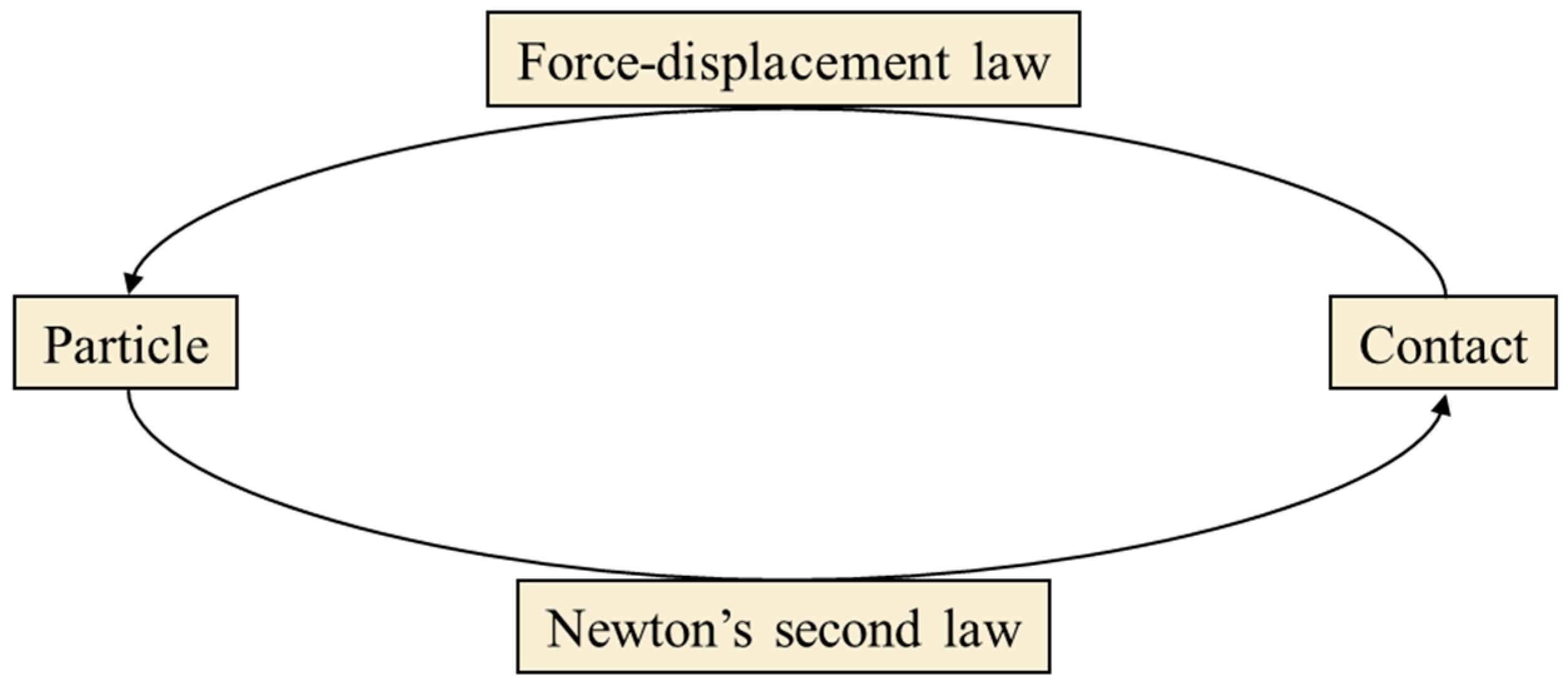
2.1. Distinct Element Method
2.2. SFLOW Model
3. Application to a Reservoir Area Case
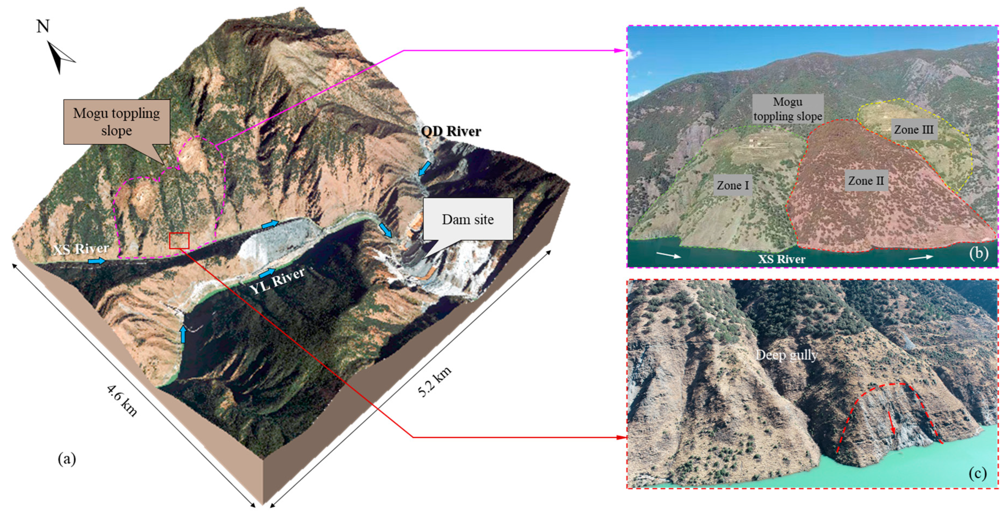
3.1. Overview of the Mogu Toppling Slope
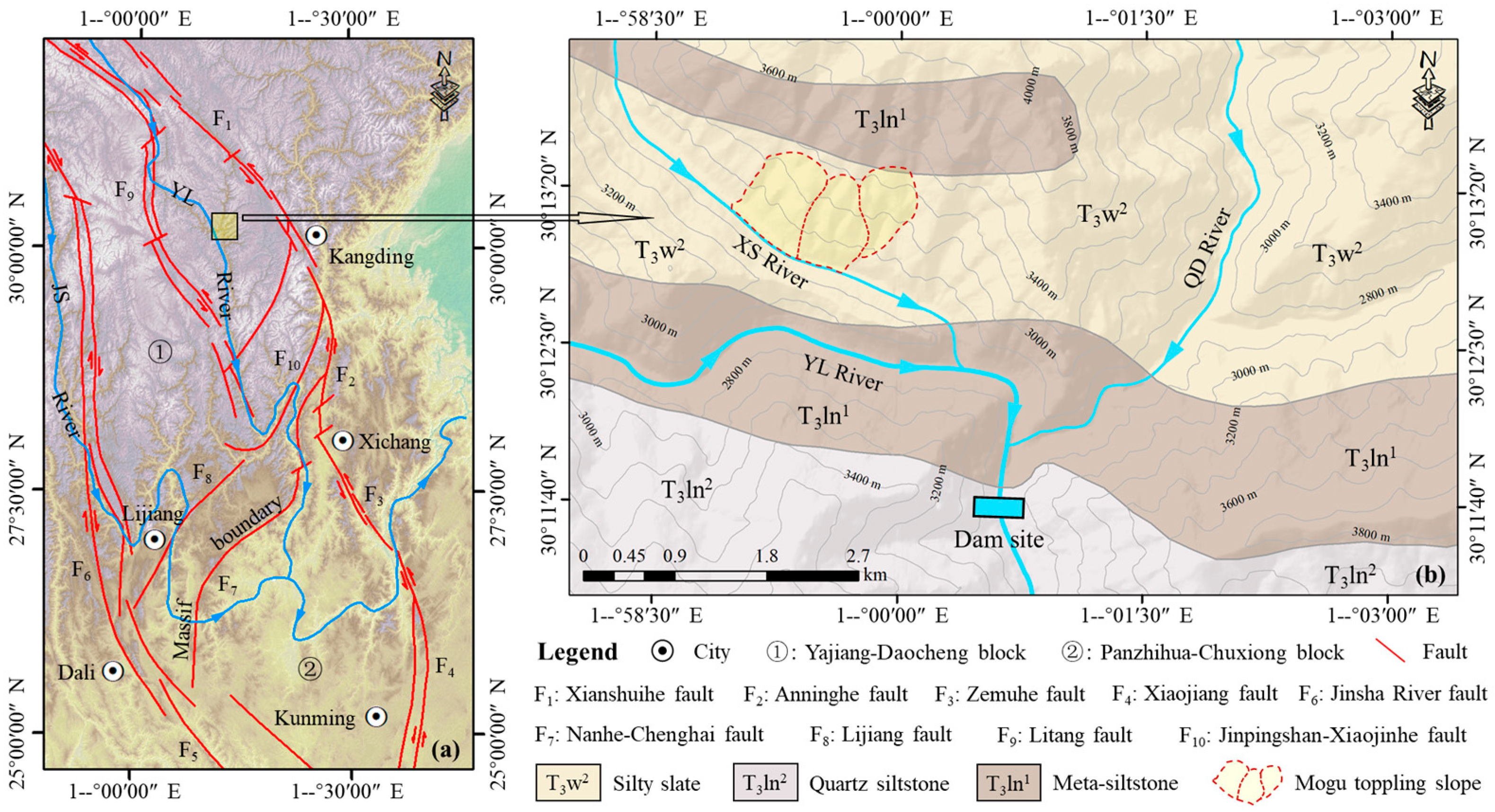
3.1.1. Geographical Setting and Engineering Background
3.1.2. Geological Setting and Slope Deformation Mechanism
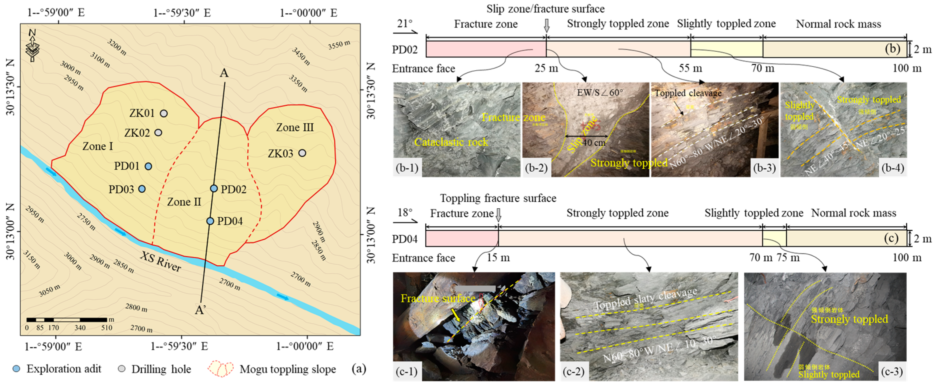
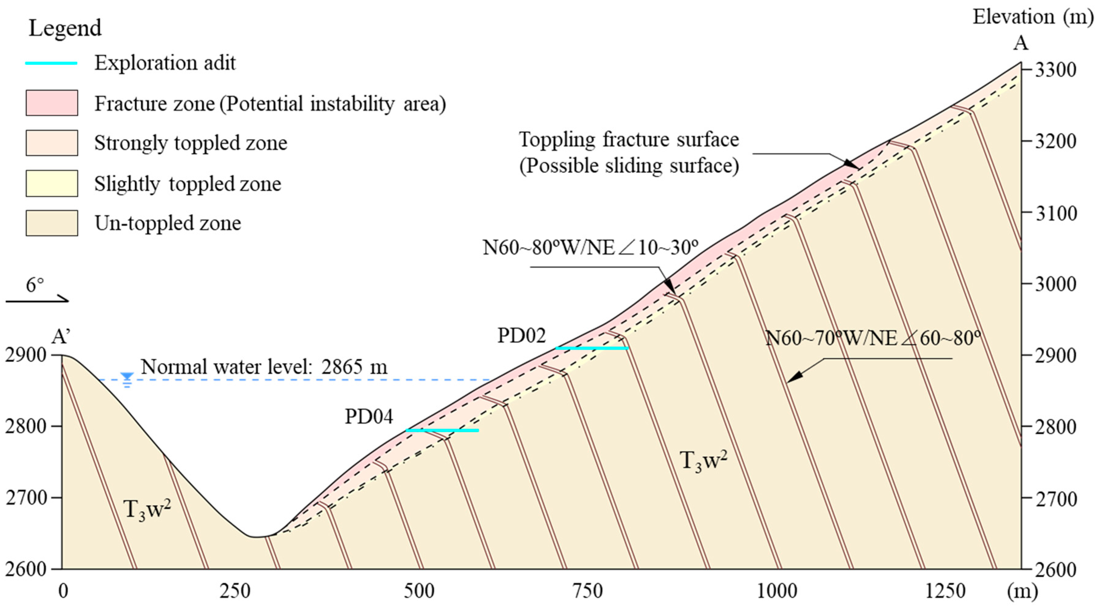
3.1.3. Toppling Zonation and Potential Instability Area
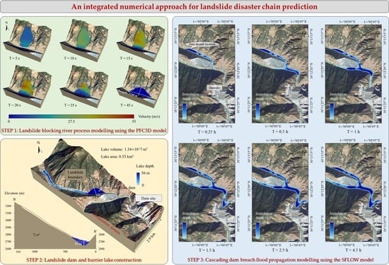
3.2. Landslide Blocking River Process Modeling
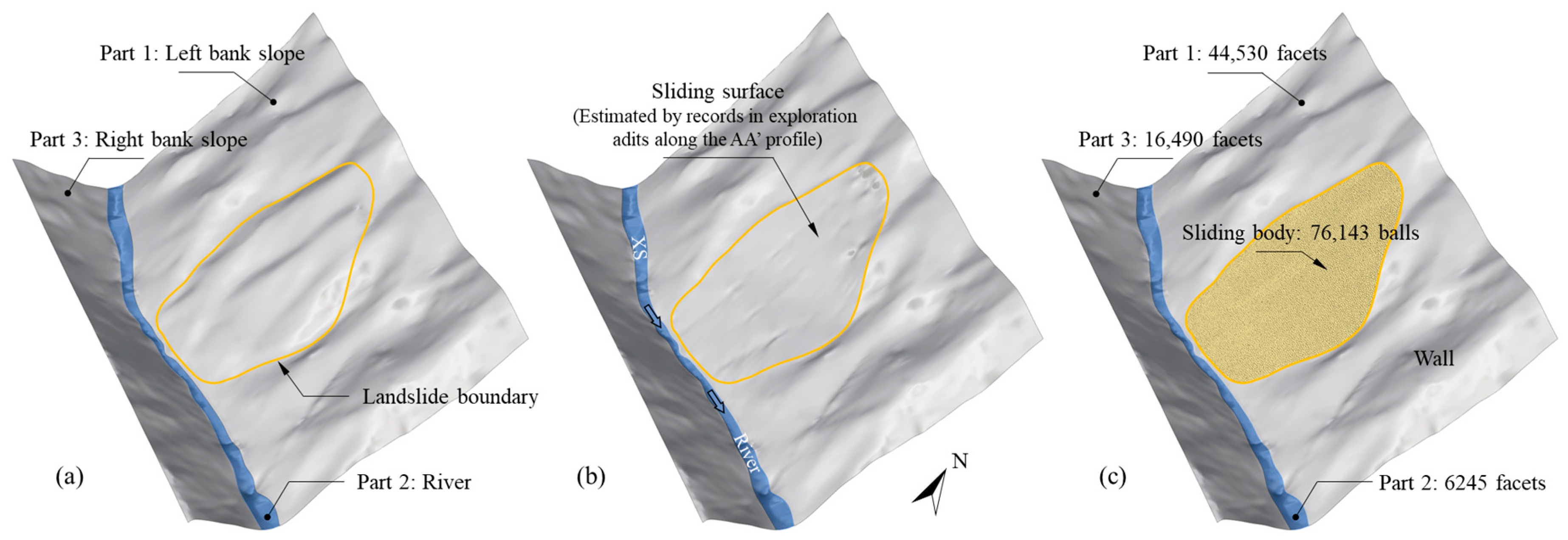
3.2.1. Construction of the Landslide Numerical Model
3.2.2. Macro-Parameters and Micro-Parameters
3.2.3. Runout Behavior and Landslide Dam Predictions
3.3. Dam Breach Flood Propagation Modelling
3.3.1. Parameters and Data Preprocessing
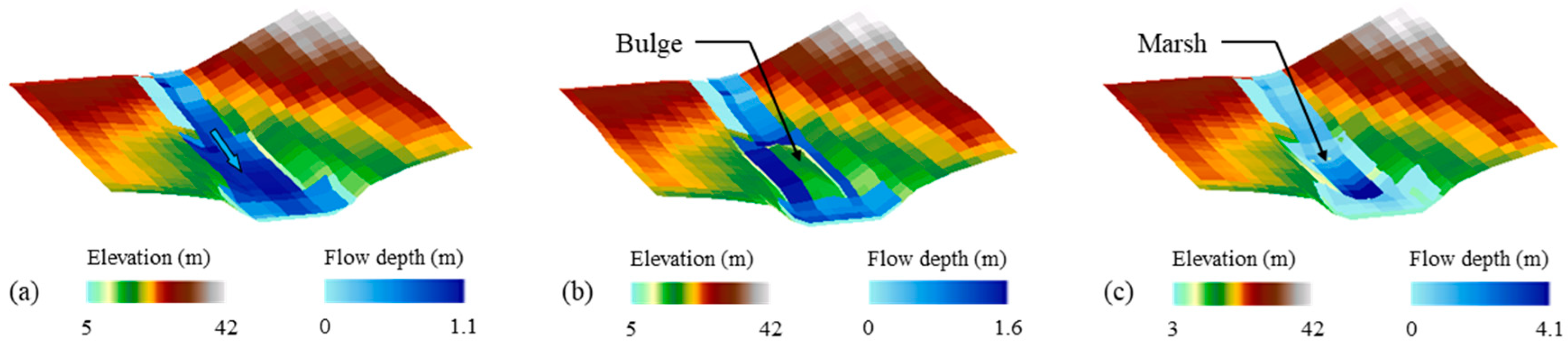
3.3.2. Flood Propagation Predictions
4. Discussion
4.1. Effect of the Friction Coefficient of the Sliding Surface
4.2. Effect of the Breach Depth
4.3. Limitations of the PFC 3D Model and the SFLOW Model
5. Conclusions
Author Contributions
Funding
Data Availability Statement
Conflicts of Interest
References
- Zhan, J.; Chen, J.; Zhang, W.; Han, X.; Sun, X.; Bao, Y. Mass movements along a rapidly uplifting river valley: An example from the upper Jinsha River, southeast margin of the Tibetan Plateau. Environ. Earth Sci. 2018, 77, 634. [Google Scholar] [CrossRef]
- Li, Z.; Chen, J.; Shan, Z.; Bao, Y.; Li, Y.; Shan, K.; Liu, D.; Han, M. Quantifying the late Quaternary incision rate in the upper Jinsha River with dated fluvial terraces and transient tributary profiles. CATENA 2023, 232, 107446. [Google Scholar] [CrossRef]
- Hu, Y.X.; Yu, Z.Y.; Zhou, J.W. Numerical simulation of landslide-generated waves during the 11 October 2018 Baige landslide at the Jinsha River. Landslides 2020, 17, 2317–2328. [Google Scholar] [CrossRef]
- Zhuang, Y.; Yin, Y.; Xing, A.; Jin, K. Combined numerical investigation of the Yigong rock slide-debris avalanche and subsequent dam-break flood propagation in Tibet, China. Landslides 2020, 17, 2217–2229. [Google Scholar] [CrossRef]
- Fan, X.; Yang, F.; Subramanian, S.S.; Xu, Q.; Feng, Z.; Mavrouli, O.; Peng, M.; Ouyang, C.; Jansen, J.D.; Huang, R. Prediction of a multi-hazard chain by an integrated numerical simulation approach: The Baige landslide, Jinsha River, China. Landslides 2020, 17, 147–164. [Google Scholar] [CrossRef]
- McDougall, S. Landslide runout analysis—Current practice and challenges. Can. Geotech. J. 2016, 54, 605–620. [Google Scholar] [CrossRef]
- Zhou, J.W.; Huang, K.X.; Shi, C.; Hao, M.H.; Guo, C.X. Discrete element modeling of the mass movement and loose material supplying the gully process of a debris avalanche in the Bayi Gully, Southwest China. J. Asian Earth Sci. 2015, 99, 95–111. [Google Scholar] [CrossRef]
- Zhan, W.; Fan, X.; Huang, R.; Pei, X.; Xu, Q.; Li, W. Empirical prediction for travel distance of channelized rock avalanches in the Wenchuan earthquake area. Nat. Hazards Earth Syst. Sci. 2017, 17, 833–844. [Google Scholar] [CrossRef]
- Scaringi, G.; Fan, X.; Xu, Q.; Liu, C.; Ouyang, C.; Domènech, G.; Yang, F.; Dai, L. Some considerations on the use of numerical methods to simulate past landslides and possible new failures: The case of the recent Xinmo landslide (Sichuan, China). Landslides 2018, 15, 1359–1375. [Google Scholar] [CrossRef]
- Yang, Q.Q.; Cai, F.; Ugai, K.; Yamada, M.; Su, Z.; Ahmed, A.; Huang, R.; Xu, Q. Some factors affecting the frontal velocity of rapid dry granular flows in a large flume. Eng. Geol. 2011, 122, 249–260. [Google Scholar] [CrossRef]
- Wang, Y.F.; Xu, Q.; Cheng, Q.G.; Li, Y.; Luo, Z.X. Spreading and deposit characteristics of a rapid dry granular avalanche across 3D topography: Experimental study. Rock Mech. Rock Eng. 2016, 49, 4349–4370. [Google Scholar] [CrossRef]
- Nian, T.K.; Wu, H.; Li, D.Y.; Zhao, W.; Takara, K.; Zheng, D.F. Experimental investigation on the formation process of landslide dams and a criterion of river blockage. Landslides 2020, 17, 2547–2562. [Google Scholar] [CrossRef]
- Yan, J.; Chen, J.; Zhou, F.; Li, Y.; Zhang, Y.; Gu, F.; Zhang, Y.; Li, Y.; Li, Z.; Bao, Y.; et al. Numerical simulation of the Rongcharong paleolandslide river-blocking event: Implication for the longevity of the landslide dam. Landslides 2022, 19, 1339–1356. [Google Scholar] [CrossRef]
- Zhang, M.; Wu, L.; Zhang, J.; Li, L. The 2009 Jiweishan rock avalanche, Wulong, China: Deposit characteristics and implications for its fragmentation. Landslides 2019, 16, 893–906. [Google Scholar] [CrossRef]
- Bao, Y.; Sun, X.; Zhou, X.; Zhang, Y.; Liu, Y. Some numerical approaches for landslide river blocking: Introduction, simulation, and discussion. Landslides 2021, 18, 3907–3922. [Google Scholar] [CrossRef]
- Gao, H.Y.; Gao, Y.; Li, B.; Yin, Y.P.; Yang, C.S.; Wan, J.W.; Zhang, T.T. The dynamic simulation and potential hazards analysis of the Yigong landslide in Tibet, China. Remote Sens. 2023, 15, 1322. [Google Scholar] [CrossRef]
- Wu, H.; Nian, T.K.; Shan, Z.G.; Li, D.Y.; Guo, X.S.; Jiang, X.G. Rapid prediction models for 3D geometry of landslide dam considering the damming process. J. Mt. Sci. 2023, 20, 928–942. [Google Scholar] [CrossRef]
- Zhu, Q.Y.; Jiang, N.; Chen, Q.; Hu, Y.X.; Zhou, J.W. DEM-SPH simulation for the formation and breaching of a landslide-dammed lake triggered by the 2022 Lushan earthquake. Landslides 2023, 20, 1925–1941. [Google Scholar] [CrossRef]
- Tang, C.; Hu, J.; Lin, M.; Angelier, J.; Lu, C.; Chan, Y.; Chu, H. The Tsaoling landslide triggered by the Chi-Chi earthquake, Taiwan: Insights from a discrete element simulation. Eng. Geol. 2009, 106, 1–19. [Google Scholar] [CrossRef]
- Lu, C.; Tang, C.; Chan, Y.; Hu, J.; Chi, C. Forecasting landslide hazard by the 3D discrete element method: A case study of the unstable slope in the Lushan hot spring district, central Taiwan. Eng. Geol. 2014, 183, 14–30. [Google Scholar] [CrossRef]
- Lin, C.; Lin, M. Evolution of the large landslide induced by typhoon Morakot: A case study in the Butangbunasi River, southern Taiwan using the discrete element method. Eng. Geol. 2015, 197, 172–187. [Google Scholar] [CrossRef]
- Bao, Y.; Zhai, S.; Chen, J.; Xu, P.; Sun, X.; Zhan, J.; Zhang, W.; Zhou, X. The evolution of the Samaoding paleolandslide river blocking event at the upstream reaches of the Jinsha River Tibetan Plateau. Geomorphology 2020, 351, 106970. [Google Scholar] [CrossRef]
- Liu, Z.; Su, L.; Zhang, C.; Iqbal, J.; Hu, B.; Dong, Z. Investigation of the dynamic process of the Xinmo landslide using the discrete element method. Comput. Geotech. 2020, 123, 103561. [Google Scholar] [CrossRef]
- Zhong, Q.; Wang, L.; Chen, S.; Chen, Z.; Shan, Y.; Zhang, Q.; Ren, Q.; Mei, S.; Jiang, J.; Hu, L.; et al. Breaches of embankment and landslide dams—State of the art review. Earth-Sci. Rev. 2021, 216, 103597. [Google Scholar] [CrossRef]
- Costa, J.E. Floods from Dam Failures: US Geological Survey Open-File Report; No. 85–560; U.S. Geological Survey: Reston, VA, USA, 1985; p. 54. [Google Scholar]
- Evans, S.G. The maximum discharge of outburst floods caused by the breaching of man-made and natural dams. Can. Geotech. J. 1986, 23, 385–387. [Google Scholar] [CrossRef]
- Costa, J.E.; Schuster, R.L. The formation and failure of natural dams. Geol. Soc. Am. Bull. 1988, 100, 1054–1068. [Google Scholar] [CrossRef]
- Walder, J.S.; O’Connor, J.E. Methods for predicting peak discharge of floods caused by failure of natural and constructed earthen dams. Water Resour. Res. 1997, 33, 2337–2348. [Google Scholar] [CrossRef]
- Peng, M.; Zhang, L.M. Breaching parameters of landslide dams. Landslides 2012, 9, 13–31. [Google Scholar] [CrossRef]
- Wu, W. Simplified physically based model of earthen embankment breaching. J. Hydraul. Eng. 2013, 139, 837–851. [Google Scholar] [CrossRef]
- Chen, Z.; Ma, L.; Yu, S.; Chen, S.J.; Zhou, X.B.; Sun, P.; Li, X. Back analysis of the draining process of the Tangjiashan barrier lake. J. Hydraul. Eng. 2015, 14, 05014011. [Google Scholar] [CrossRef]
- Zhong, Q.M.; Chen, S.S.; Mei, S.A.; Cao, W. Numerical simulation of landslide dam breaching due to overtopping. Landslides 2018, 15, 1183–1192. [Google Scholar] [CrossRef]
- Wang, B.; Yang, S.; Chen, C. Landslide dam breaching and outburst floods: A numerical model and its application. J. Hydrol. 2022, 609, 127733. [Google Scholar] [CrossRef]
- Shrestha, B.B.; Nakagawa, H. Hazard assessment of the formation and failure of the Sunkoshi landslide dam in Nepal. Nat. Hazards 2016, 82, 2029–2049. [Google Scholar] [CrossRef]
- Zhang, Y.; Chen, J.; Zhou, F.; Bao, Y.; Yan, J.; Zhang, Y.; Li, Y.; Gu, F.; Wang, Q. Combined numerical investigation of the Gangda paleolandslide runout and associated dam breach flood propagation in the upper Jinsha River, SE Tibetan Plateau. Landslides 2022, 19, 941–962. [Google Scholar] [CrossRef]
- Li, M.H.; Sung, R.T.; Dong, J.J.; Lee, C.T.; Chen, C.C. The formation and breaching of a short-lived landslide dam at Hsiaolin village, Taiwan—Part II: Simulation of debris flow with landslide dam breach. Eng. Geol. 2011, 123, 60–71. [Google Scholar] [CrossRef]
- Liu, Y.; Zhou, J.; Song, L.; Zou, Q.; Liao, L.; Wang, Y. Numerical modelling of free-surface shallow flows over irregular topography with complex geometry. Appl. Math. Model. 2013, 37, 9482–9498. [Google Scholar] [CrossRef]
- Wang, W.; Chen, W.; Huang, G. Research on flood propagation for different dam failure modes: A case study in Shenzhen, China. Front. Earth Sci. 2020, 8, 527363. [Google Scholar] [CrossRef]
- Song, L.; Zhou, J.; Guo, J.; Zou, Q.; Liu, Y. A robust well-balanced finite volume model for shallow water flows with wetting and drying over irregular terrain. Adv. Water Resour. 2011, 34, 915–932. [Google Scholar] [CrossRef]
- Pongsanguansin, T.; Maleewong, M.; Mekchay, K. Shallow-water simulations by a well-balanced WAF finite volume method: A case study to the great flood in 2011, Thailand. Comput. Geosci. 2016, 20, 1269–1285. [Google Scholar] [CrossRef]
- Han, X.; Chen, J.; Xu, P.; Zhan, J. A well-balanced numerical scheme for debris flow run-out prediction in Xiaojia Gully considering different hydrological designs. Landslides 2017, 14, 2105–2114. [Google Scholar] [CrossRef]
- Bao, Y.; Chen, J.; Sun, X.; Han, X.; Li, Y.; Zhang, Y.; Gu, F.; Wang, J. Debris flow prediction and prevention in reservoir area based on finite volume type shallow-water model: A case study of pumped-storage hydroelectric power station site in Yi County, Hebei, China. Environ. Earth Sci. 2019, 78, 577. [Google Scholar] [CrossRef]
- Poisel, R.; Angerer, H.; Pöllinger, M.; Kalcher, T.; Kittl, H. Mechanics and velocity of the Lärchberg-Galgenwald landslide (Austria). Eng. Geol. 2009, 109, 57–66. [Google Scholar] [CrossRef]
- Wang, S.; Xu, W.; Shi, C.; Chen, H. Run-out prediction and failure mechanism analysis of the Zhenggang deposit in southwestern China. Landslides 2017, 14, 719–726. [Google Scholar] [CrossRef]
- Cundall, P.A. A computer model for simulating progressive large scale movements in blocky rock systems. In Proceedings of the Symposium of the International Society for Rock Mechanics, Society for Rock Mechanics (ISRM), Nancy, France, 4–6 October 1971. [Google Scholar]
- Cundall, P.; Strack, O. A discrete numerical model for granular assemblies. Geotechnique 1979, 29, 47–65. [Google Scholar] [CrossRef]
- Wei, J.; Zhao, Z.; Xu, C.; Wen, Q. Numerical investigation of landslide kinetics for the recent Mabian landslide (Sichuan, China). Landslides 2019, 16, 2287–2298. [Google Scholar] [CrossRef]
- Li, W.; Li, H.; Dai, F.; Lee, L. Discrete element modeling of a rainfall-induced flowslide. Eng. Geol. 2012, 149–150, 22–34. [Google Scholar] [CrossRef]
- Lo, C.M.; Lin, M.L.; Tang, C.L.; Hu, J.C. A kinematic model of the Hsiaolin landslide calibrated to the morphology of the landslide deposit. Eng. Geol. 2011, 123, 22–39. [Google Scholar] [CrossRef]
- Potyondy, D.; Cundall, P. A bonded-particle model for rock. Int. J. Rock Mech. Min. 2004, 41, 1329–1364. [Google Scholar] [CrossRef]
- Zhai, S.; Zhan, J.; Bao, Y.; Chen, J.; Li, Y.; Li, Z. PFC model parameter calibration using uniform experimental design and a deep learning network. IOP Conf. Ser. Earth Environ. Sci. 2019, 304, 032062. [Google Scholar] [CrossRef]
- Wu, N.J.; Chen, C.; Tsay, T.K. Application of weighted-least-square local polynomial approximation to 2d shallow-water equation problems. Eng. Anal. Bound. Elem. 2016, 68, 124–134. [Google Scholar] [CrossRef]
- Chen, H.X.; Zhang, L.M.; Gao, L.; Yuan, Q.; Lu, T.; Xiang, B.; Zhang, W.L. Simulation of interactions among multiple debris flows. Landslides 2017, 14, 595–615. [Google Scholar] [CrossRef]
- Liang, Q.H. Flood simulation using a well-balanced shallow flow model. J. Hydraul. Eng. 2010, 136, 669–675. [Google Scholar] [CrossRef]
- Liang, Q.; Marche, F. Numerical resolution of well-balanced shallow water equations with complex source terms. Adv. Water Resour. 2009, 32, 873–884. [Google Scholar] [CrossRef]
- Tu, G.; Deng, H.; Shang, Q.; Zhang, Y.; Luo, X. Deep-seated large-scale toppling failure: A case study of the Lancang slope in southwest China. Rock Mech. Rock Eng. 2020, 53, 3417–3432. [Google Scholar] [CrossRef]
- Zhao, W.; Zhang, C.; Ju, N. Identification and zonation of deep-seated toppling deformation in a metamorphic rock slope. Bull. Eng. Geol. Environ. 2021, 80, 1981–1997. [Google Scholar] [CrossRef]
- Xu, W.Y.; Qin, C.C.; Zhang, G.K.; Deng, S.H.; Hu, Y.F.; Zhang, H.L. Calculation method for far-field propagation of landslide surge based on flow diversion ratio of a bifurcated river. Adv. Sci. Technol. Water Resour. 2022, 42, 20–24. [Google Scholar] [CrossRef]
- Tang, S.; Wang, J.; Chen, P. Theoretical and numerical studies of cryogenic fracturing induced by thermal shock for reservoir stimulation. Int. J. Rock Mech. Min. 2020, 125, 104160. [Google Scholar] [CrossRef]
- Tai, D.; Qi, S.; Zheng, B.; Wang, C.; Guo, S.; Luo, G. Shear mechanical properties and energy evolution of rock-like samples containing multiple combinations of non-persistent joints. J. Rock Mech. Geotech. Eng. 2023, 15, 1651–1670. [Google Scholar] [CrossRef]
- Ma, W.; Chen, H.; Zhang, W.; Tan, C.; Nie, Z.; Wang, J.; Sun, Q. Study on representative volume elements considering inhomogeneity and anisotropy of rock masses characterised by non-persistent fractures. Rock Mech. Rock Eng. 2021, 54, 4617–4637. [Google Scholar] [CrossRef]
- Campbell, C.S. Self-lubrication for long runout landslides. J. Geol. 1989, 97, 653–665. [Google Scholar] [CrossRef]
- Aaron, J.; Hungr, O. Dynamic analysis of an extraordinarily mobile rock avalanche in the Northwest Territories, Canada. Can. Geotech. J. 2016, 53, 899–908. [Google Scholar] [CrossRef]
- Aaron, J.; McDougall, S. Rock avalanche mobility: The role of path material. Eng. Geol. 2019, 257, 105–126. [Google Scholar] [CrossRef]
- Hungr, O.; Leroueil, S.; Picarelli, L. The Varnes classification of landslide types, an update. Landslides 2014, 11, 167–194. [Google Scholar] [CrossRef]
- Zhou, J.W.; Cui, P.; Fang, H. Dynamic process analysis for the formation of Yangjiagou landslide-dammed lake triggered by the Wenchuan earthquake, China. Landslides 2013, 10, 331–342. [Google Scholar] [CrossRef]
- Liu, W.; Carling, P.A.; Hu, K.; Wang, H.; Zhou, Z.; Zhou, L.; Liu, D.; Lai, Z.; Zhang, X. Outburst floods in China: A review. Earth-Sci. Rev. 2019, 197, 102895. [Google Scholar] [CrossRef]
- Fan, X.; Dufresne, A.; Subramanian, S.S.; Strom, A.; Hermanns, R.; Stefanelli, C.T.; Hewitt, K.; Yunus, A.P.; Dunning, S.; Capra, L.; et al. The formation and impact of landslide dams—State of the art. Earth-Sci. Rev. 2020, 203, 103116. [Google Scholar] [CrossRef]
- O’Brien, J.S. FLO-2D User’s Manual, Version 2006.01; FLO-2D Software, Inc.: Nutrioso, AZ, USA, 2006.
- Chen, H.X.; Zhang, L.M.; Zhang, S.; Xiang, B.; Wang, X.F. Hybrid simulation of the initiation and runout characteristics of a catastrophic debris flow. J. Mt. Sci. 2013, 10, 219–232. [Google Scholar] [CrossRef]
- Sun, R.J.; Du, W.C.; Xie, M.W. Risk analysis of reservoir dam-break based on HEC-RAS and ArcGIS. J. Geomat. 2017, 42, 98–101. [Google Scholar] [CrossRef]
- Liu, J.H.; Li, Q.L.; Xue, Y.; He, Y.; Ge, C.; Guo, J. Study on instantaneous outburst flood process of dambreak. J. Water Resour. Res. 2022, 11, 93–101. [Google Scholar] [CrossRef]


| Micro-Parameter | Symbol | Numerical Direct Shear Test | Numerical Landslide Model |
|---|---|---|---|
| Linear group | |||
| Number of ball elements | 8572 | 76,143 | |
| Minimum ball radius (m) | 0.002 | 2 | |
| Ball radius ratio | / | 1.66 | 1.66 |
| Ball density (kg/m3) | 2400 | 2400 | |
| Ball friction coefficient | 0.3 | 0.3 | |
| Normal stiffness (N/m) | 8 × 10⁵~1.33 × 10⁶ | 8 × 10⁸~1.33 × 10⁹ | |
| Normal-to-shear stiffness ratio | 3 | 3 | |
| Parallel bond group | |||
| Bond normal stiffness (N/m3) | 1.51 × 10¹⁰~2.5 × 10¹⁰ | 1.51 × 10⁷~2.5 × 10⁷ | |
| Bond normal-to-shear stiffness ratio | 3 | 3 | |
| Normal strength (Pa) | 2.1 × 10⁷ | 2.1 × 10⁷ | |
| Shear strength (Pa) | 2.2 × 10⁷ | 2.2 × 10⁷ | |
| Dashpot group | |||
| Normal critical damping ratio | 0.1 | 0.1 | |
| Shear critical damping ratio | 0.1 | 0.1 |
| Reheological Parameter | Symbal | Value |
|---|---|---|
| Sediment density (kg/m3) | 1500 | |
| Sediment concentration by volume | 0.1 | |
| Yield stress (Pa) | 500 | |
| Viscosity of flood ( Pa∙s) | 0.0325 | |
| Resistance coefficient | 100 | |
| Manning resistance coefficient (s/m1/3) | 0.025 |
| Equation | Investigator | Predicted Value (m3/s) |
|---|---|---|
| Costa (1985) [25] | 5239 | |
| Evans (1986) [26] | 4311 | |
| Costa and Schuster (1988) [27] | 2979 | |
| Walder and O’Connor (1997) [28] | 3513 | |
| Peng and Zhang (2012) [29] | 1837 |
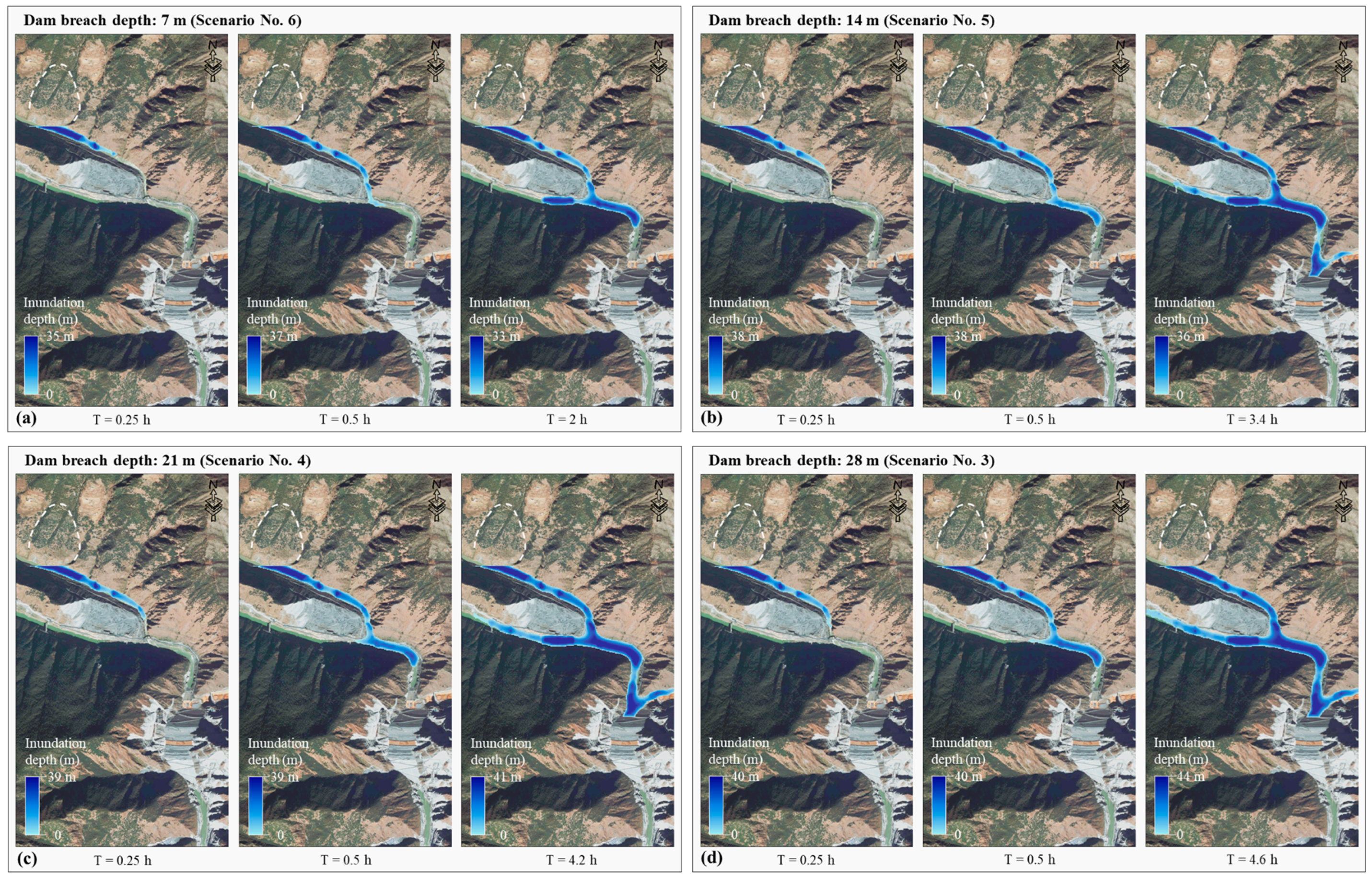
| Scenario | Dam Failure Mode | Breach Morphology (Cross-Section) | ||
|---|---|---|---|---|
| (m) | (m) | (m) | ||
| No. 1 | Complete dam-break | 56 | 186 | --- |
| No. 2 | Partial dam-break | 42 | 157 | 73 |
| No. 3 | 28 | 159 | 103 | |
| No. 4 | 21 | 165 | 123 | |
| No. 5 | 14 | 166 | 138 | |
| No. 6 | 7 | 165 | 151 | |
Disclaimer/Publisher’s Note: The statements, opinions and data contained in all publications are solely those of the individual author(s) and contributor(s) and not of MDPI and/or the editor(s). MDPI and/or the editor(s) disclaim responsibility for any injury to people or property resulting from any ideas, methods, instructions or products referred to in the content. |
© 2023 by the authors. Licensee MDPI, Basel, Switzerland. This article is an open access article distributed under the terms and conditions of the Creative Commons Attribution (CC BY) license (https://creativecommons.org/licenses/by/4.0/).
Share and Cite
Yan, J.; Xing, X.; Li, X.; Zhu, C.; Han, X.; Zhao, Y.; Chen, J. RETRACTED: Forecasting the Landslide Blocking River Process and Cascading Dam Breach Flood Propagation by an Integrated Numerical Approach: A Reservoir Area Case Study. Remote Sens. 2023, 15, 4669. https://doi.org/10.3390/rs15194669
Yan J, Xing X, Li X, Zhu C, Han X, Zhao Y, Chen J. RETRACTED: Forecasting the Landslide Blocking River Process and Cascading Dam Breach Flood Propagation by an Integrated Numerical Approach: A Reservoir Area Case Study. Remote Sensing. 2023; 15(19):4669. https://doi.org/10.3390/rs15194669
Chicago/Turabian StyleYan, Jianhua, Xiansen Xing, Xiaoshuang Li, Chun Zhu, Xudong Han, Yong Zhao, and Jianping Chen. 2023. "RETRACTED: Forecasting the Landslide Blocking River Process and Cascading Dam Breach Flood Propagation by an Integrated Numerical Approach: A Reservoir Area Case Study" Remote Sensing 15, no. 19: 4669. https://doi.org/10.3390/rs15194669
APA StyleYan, J., Xing, X., Li, X., Zhu, C., Han, X., Zhao, Y., & Chen, J. (2023). RETRACTED: Forecasting the Landslide Blocking River Process and Cascading Dam Breach Flood Propagation by an Integrated Numerical Approach: A Reservoir Area Case Study. Remote Sensing, 15(19), 4669. https://doi.org/10.3390/rs15194669