Author Contributions
Conceptualization, Y.Z. and J.Z.; methodology, J.Z.; software, Y.Z.; validation, Y.Z., K.Z. and J.Z.; formal analysis, J.Z.; investigation, Y.Z.; resources, Z.S.; data curation, Z.S.; writing—original draft preparation, Y.Z.; writing—review and editing, J.Z. and Z.S.; visualization, Y.Z.; supervision, Z.S.; project administration, Z.S.; funding acquisition, Z.S. All authors have read and agreed to the published version of the manuscript.
Figure 1.
The schematic diagram of a three-dimensional scene.
Figure 1.
The schematic diagram of a three-dimensional scene.
Figure 2.
Concentric circle distance approximation schematic diagram.
Figure 2.
Concentric circle distance approximation schematic diagram.
Figure 3.
Three-dimensional illustration depicting occlusion relationship.
Figure 3.
Three-dimensional illustration depicting occlusion relationship.
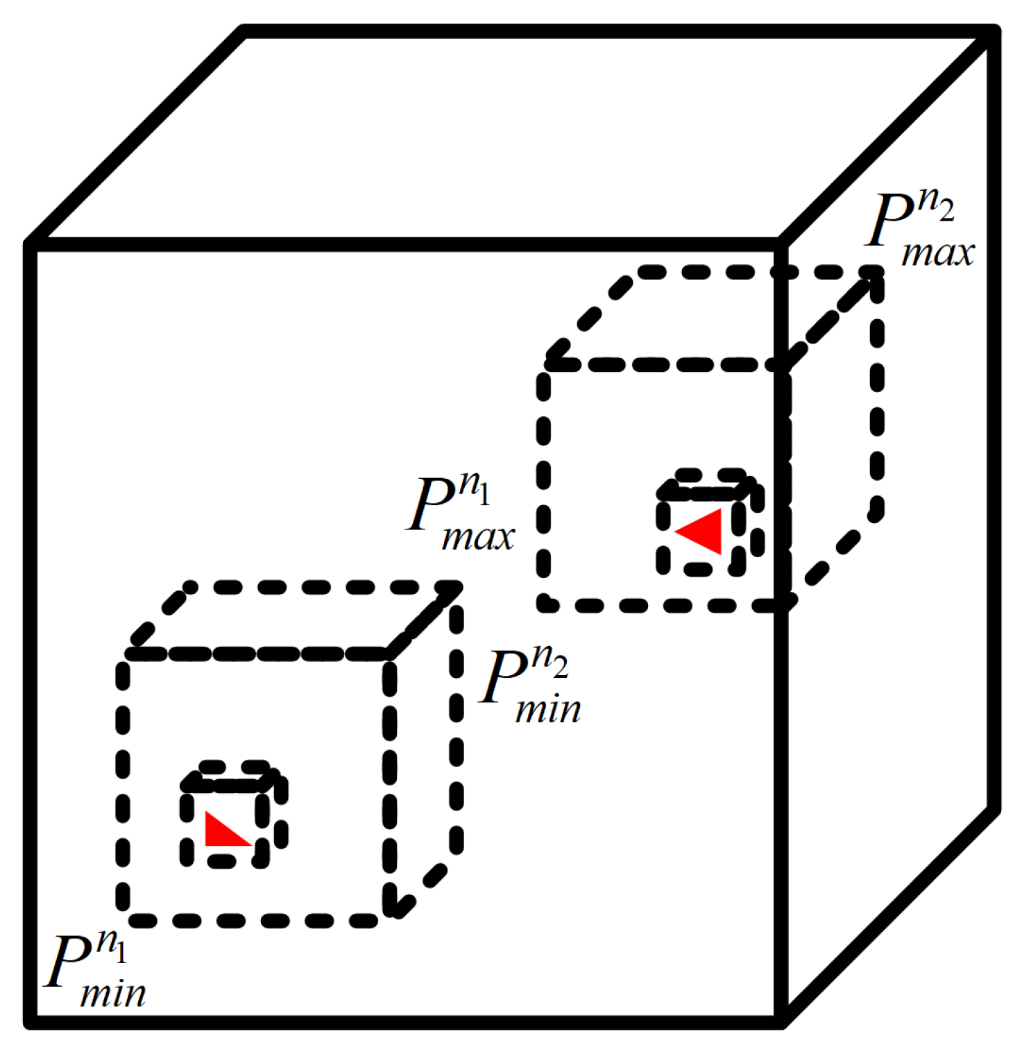
Figure 4.
Illustrative diagram for BVH structure construction.
Figure 4.
Illustrative diagram for BVH structure construction.
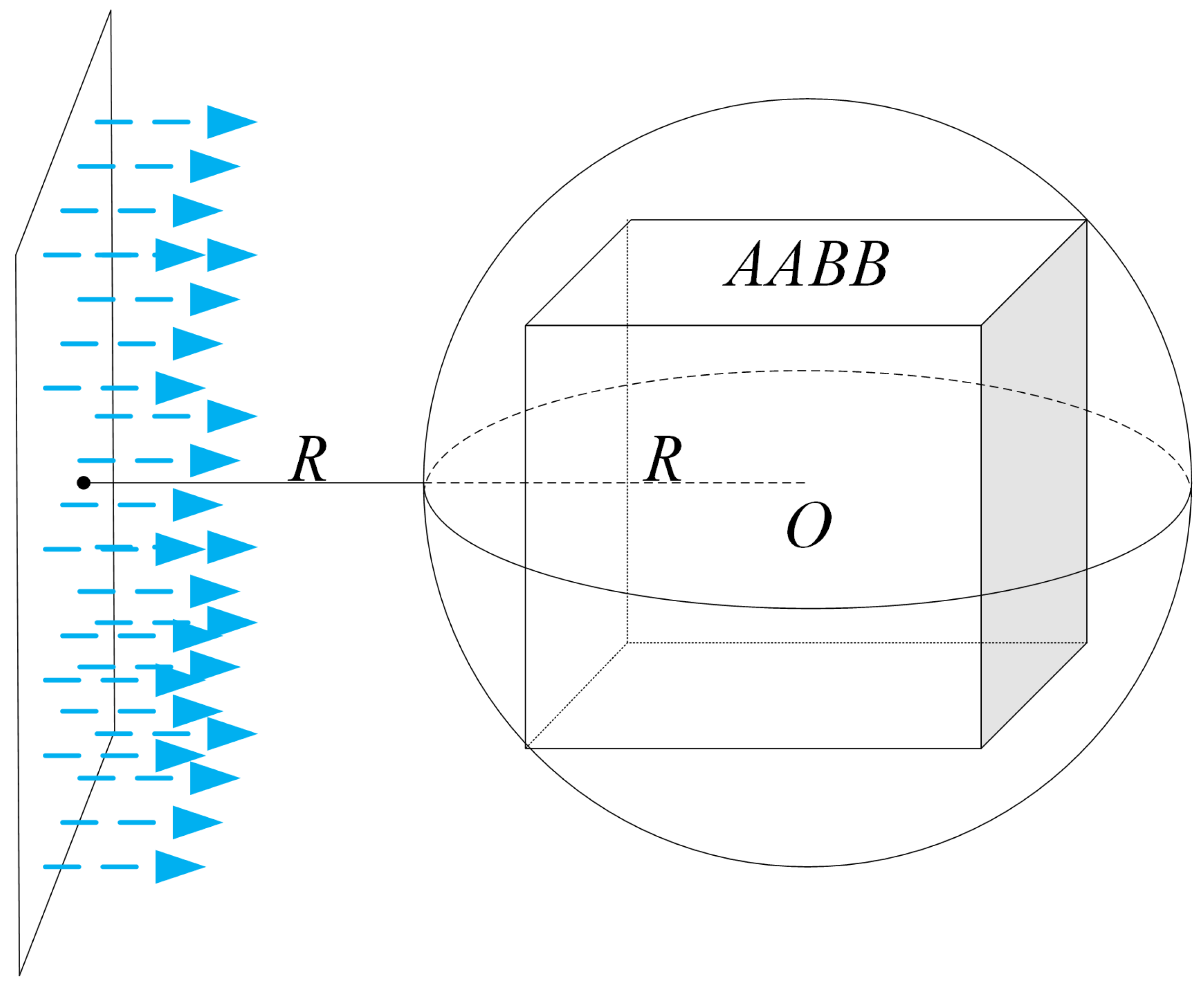
Figure 5.
Schematic diagram of the relationship between ray and AABB.
Figure 5.
Schematic diagram of the relationship between ray and AABB.
Figure 6.
The illustration of spatial relationship between the center of the ray plane and AABB.
Figure 6.
The illustration of spatial relationship between the center of the ray plane and AABB.
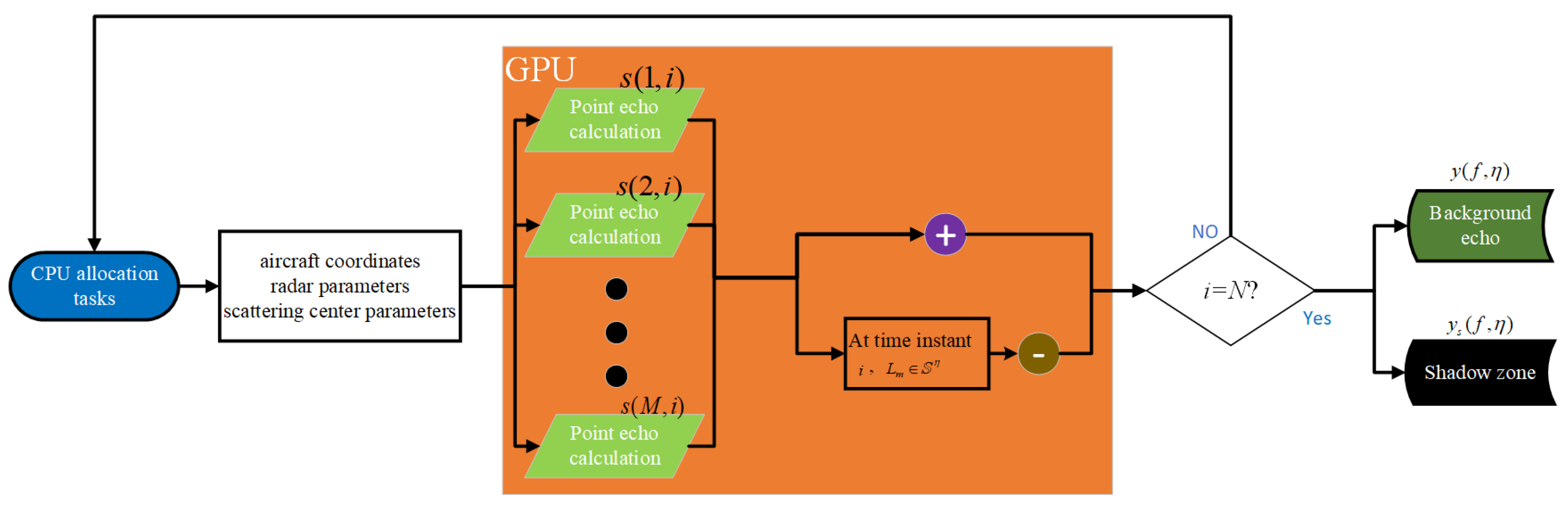
Figure 7.
A GPU-based background fast simulation workflow diagram.
Figure 7.
A GPU-based background fast simulation workflow diagram.
Figure 8.
Flowchart of GPU-based target rapid simulation algorithm.
Figure 8.
Flowchart of GPU-based target rapid simulation algorithm.
Figure 9.
GPU-based video SAR simulation algorithm workflow diagram.
Figure 9.
GPU-based video SAR simulation algorithm workflow diagram.
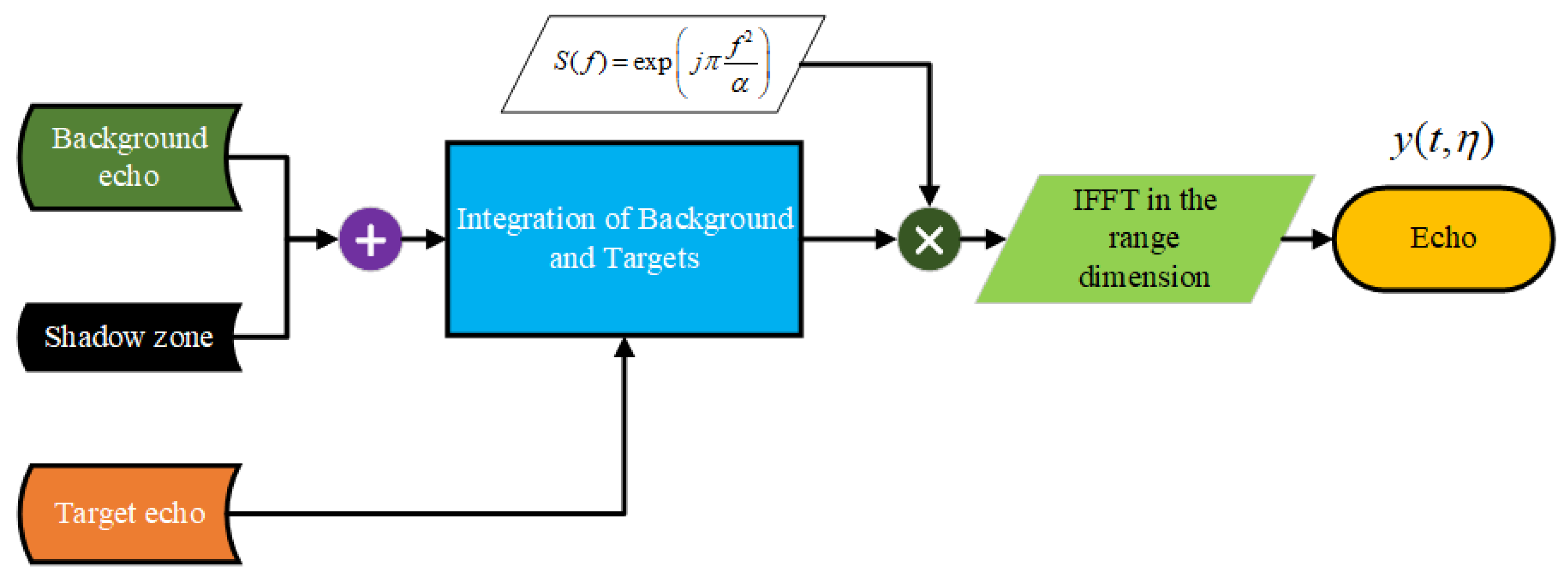
Figure 10.
Flowchart of the integration program for background and targets.
Figure 10.
Flowchart of the integration program for background and targets.
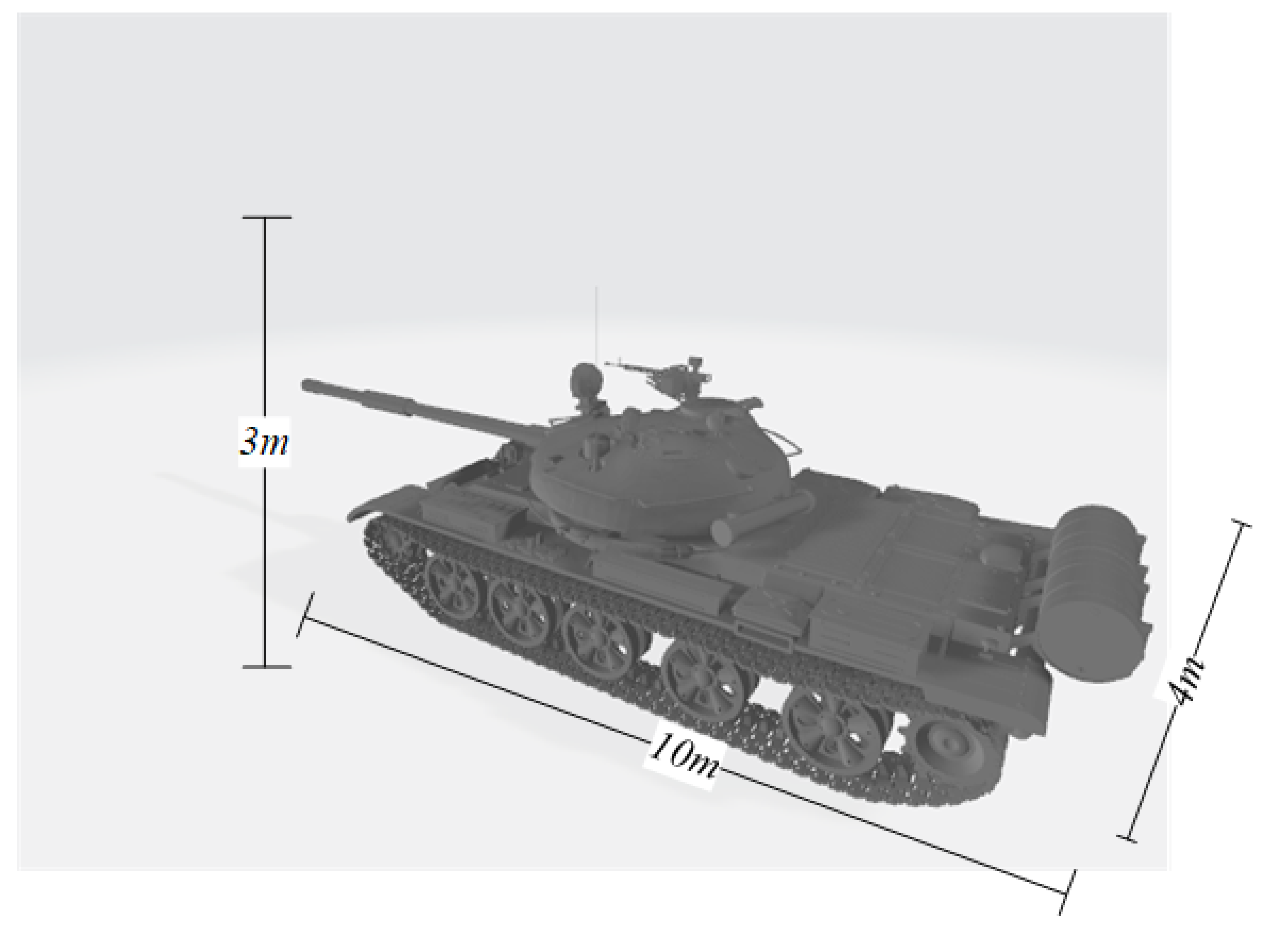
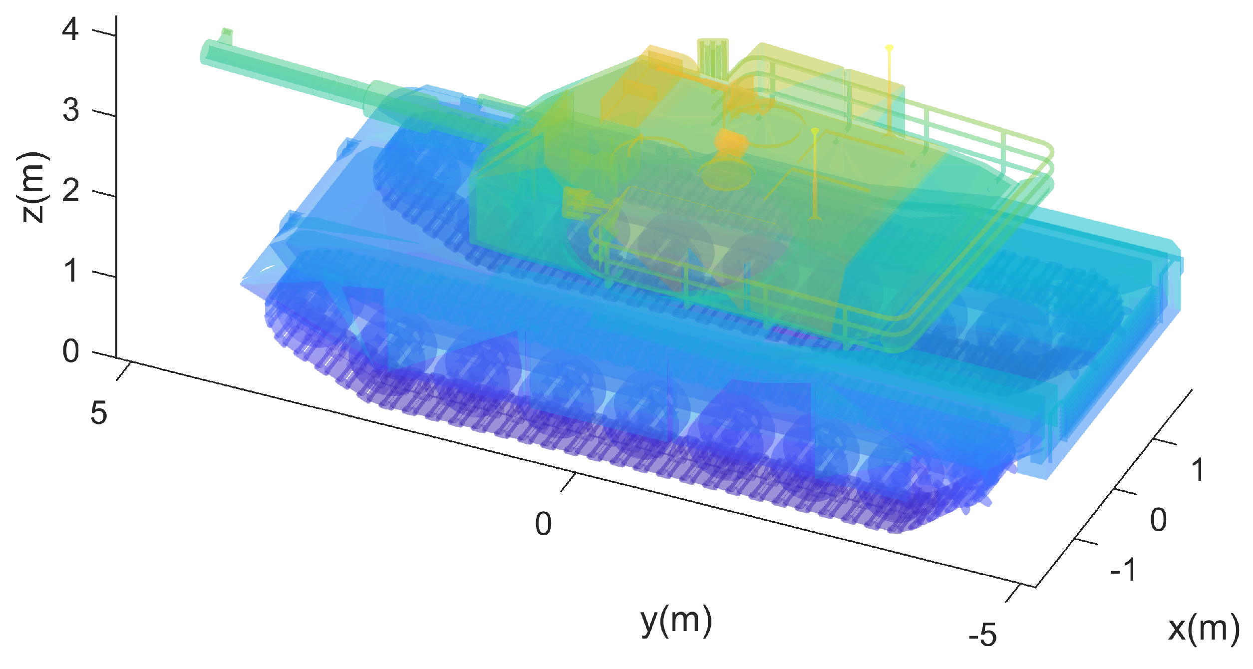
Figure 11.
The 3D model of the T62.
Figure 11.
The 3D model of the T62.
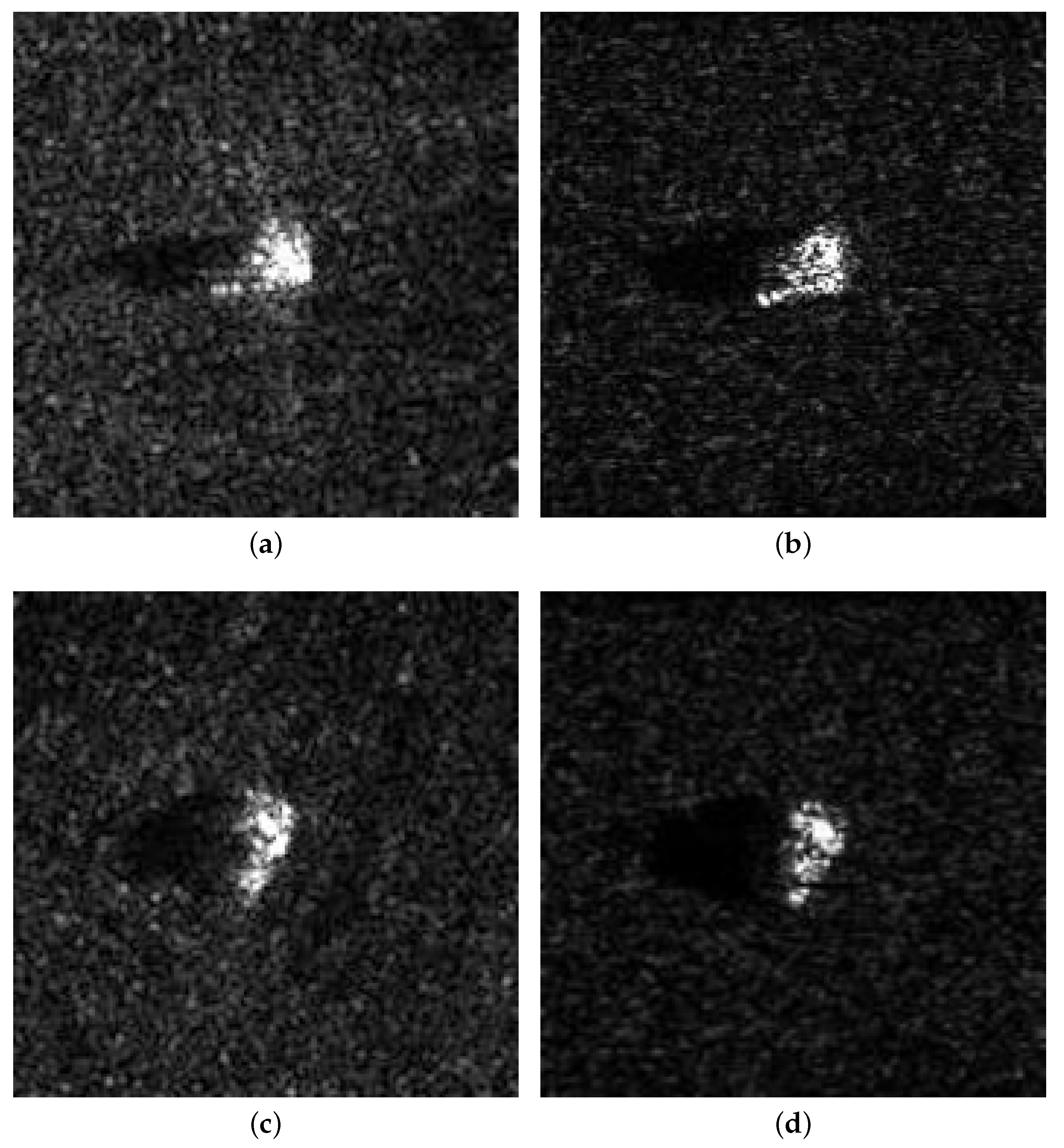
Figure 12.
Comparison between simulated image and MSTAR image. (a) MSTAR image at . (b) Simulation image at . (c) MSTAR image at . (d) Simulation image at .
Figure 12.
Comparison between simulated image and MSTAR image. (a) MSTAR image at . (b) Simulation image at . (c) MSTAR image at . (d) Simulation image at .
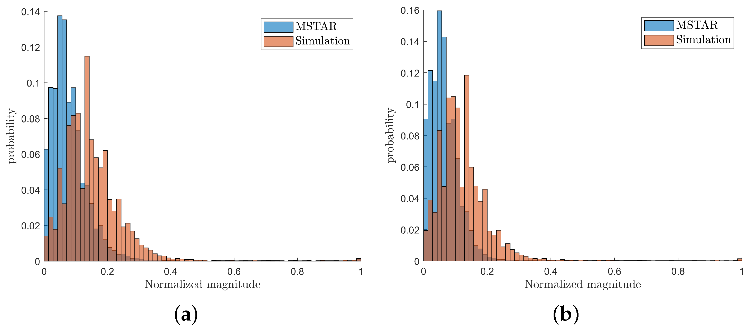
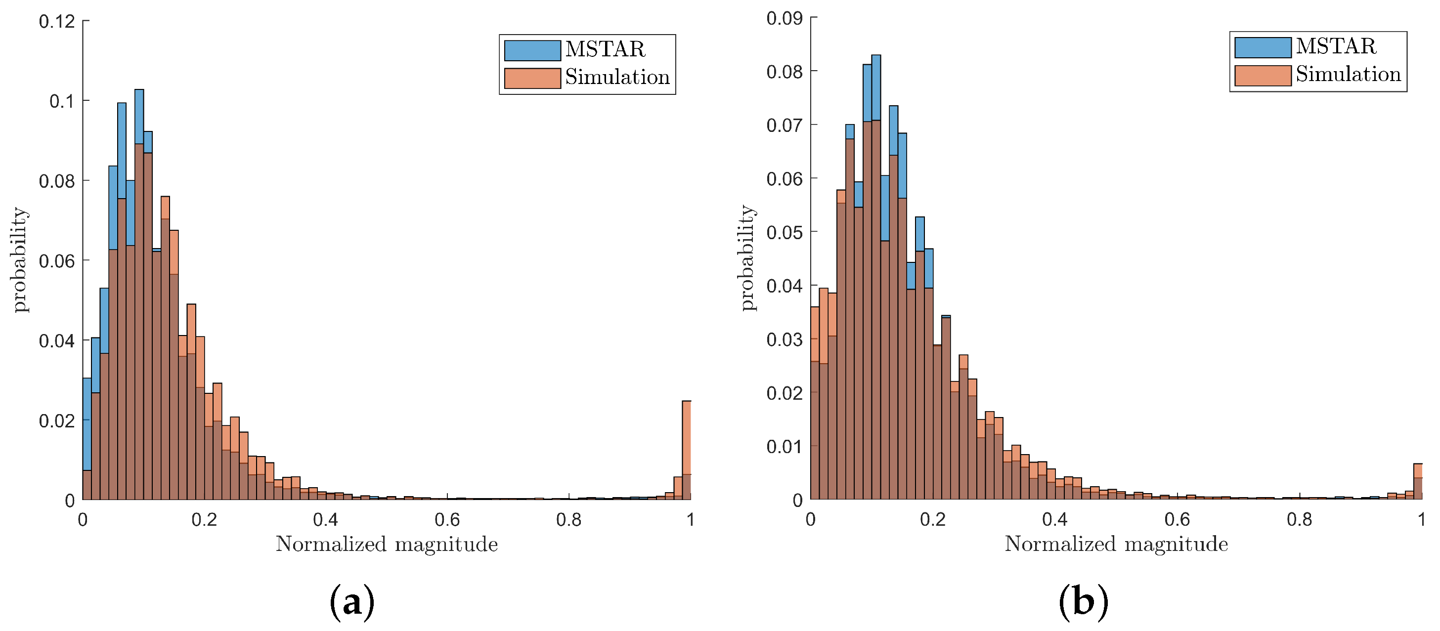
Figure 13.
Comparison of amplitude distributions between simulated images and MSTAR data. (a) Comparison of amplitude distributions between simulated image and MSTAR data at . (b) Comparison of amplitude distributions between simulated image and MSTAR data at .
Figure 13.
Comparison of amplitude distributions between simulated images and MSTAR data. (a) Comparison of amplitude distributions between simulated image and MSTAR data at . (b) Comparison of amplitude distributions between simulated image and MSTAR data at .
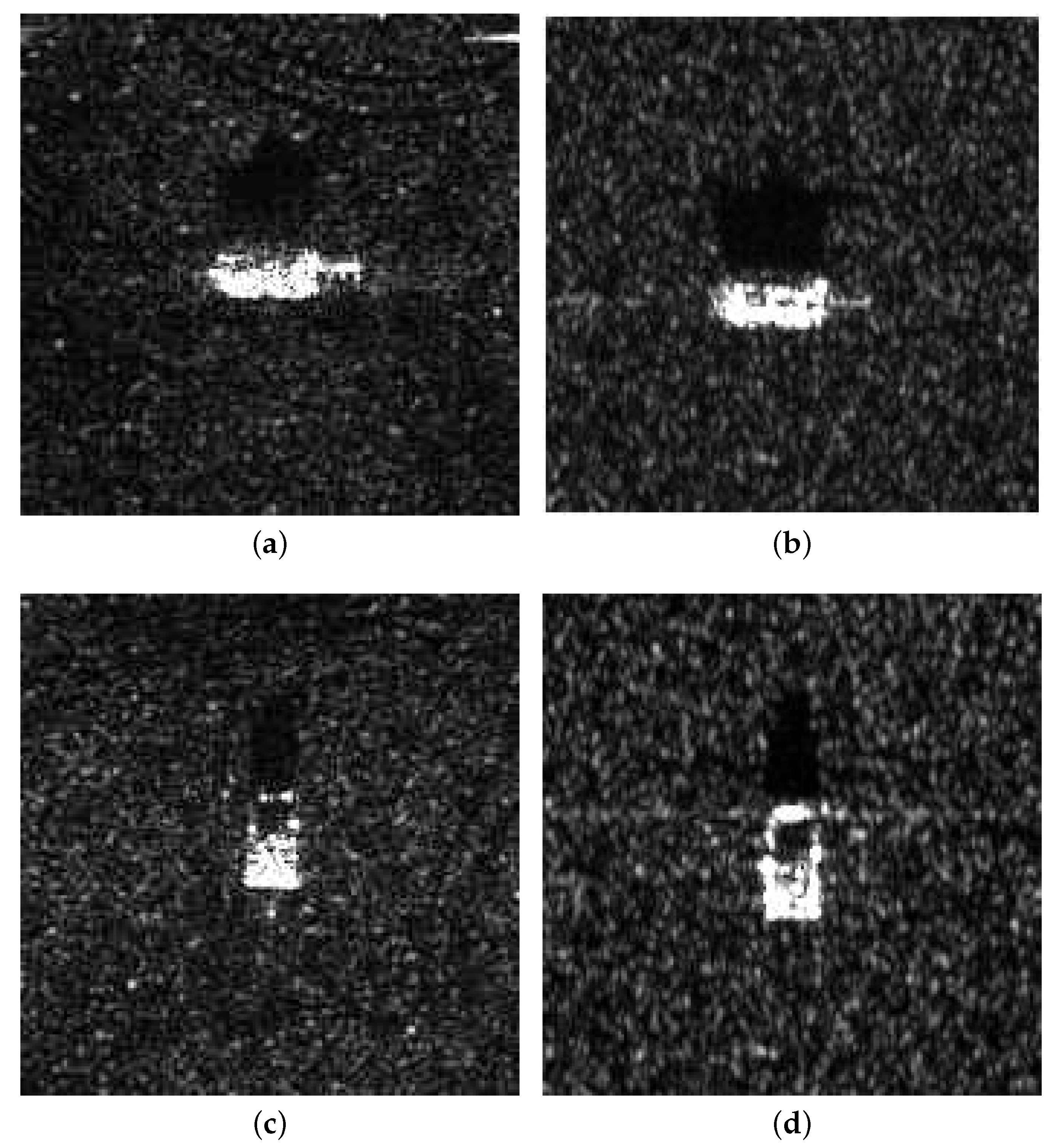
Figure 14.
Comparison between simulated image and MSTAR image. (a) MSTAR image at . (b) Simulation image at . (c) MSTAR image at . (d) Simulation image at .
Figure 14.
Comparison between simulated image and MSTAR image. (a) MSTAR image at . (b) Simulation image at . (c) MSTAR image at . (d) Simulation image at .
Figure 15.
Comparison of amplitude distributions between simulated images and MSTAR data. (a) Comparison of amplitude distributions between simulated image and MSTAR data at . (b) Comparison of amplitude distributions between simulated image and MSTAR data at .
Figure 15.
Comparison of amplitude distributions between simulated images and MSTAR data. (a) Comparison of amplitude distributions between simulated image and MSTAR data at . (b) Comparison of amplitude distributions between simulated image and MSTAR data at .
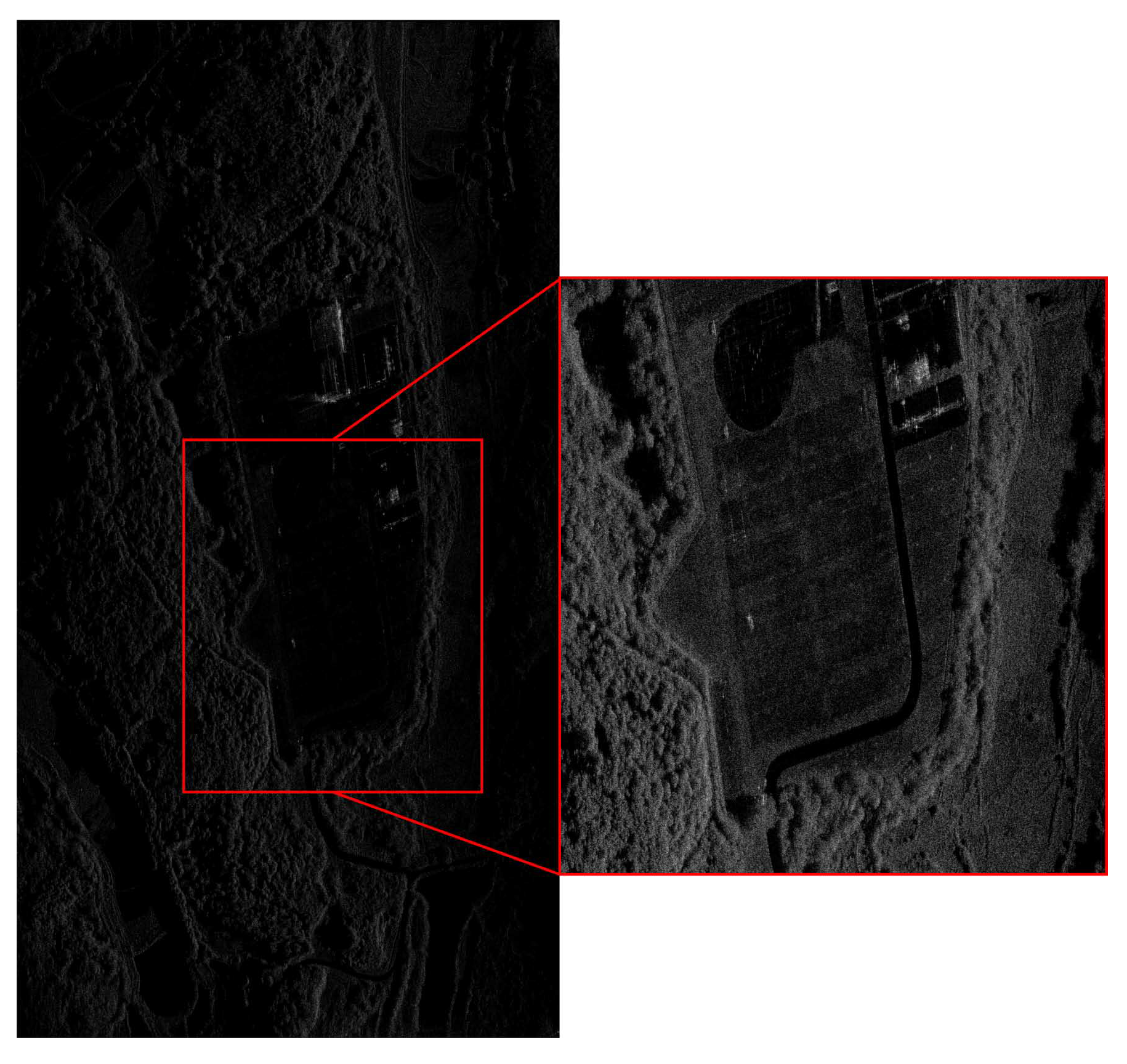
Figure 16.
Measured SAR data.
Figure 16.
Measured SAR data.
Figure 17.
Diagram of the simulated results for concentric circles. (a) Diagram of the simulated results for concentric circles at BW. (b) Diagram of the simulated results for concentric circles at BW. (c) Diagram of the simulated results for concentric circles at BW. (d) Diagram of the simulated results for concentric circles at BW.
Figure 18.
Diagram depicting the results of the magnitude distribution comparison. (a) Diagram illustrating the results of the magnitude distribution comparison at BW. (b) Diagram illustrating the results of the magnitude distribution comparison at BW. (c) Diagram illustrating the results of the magnitude distribution comparison at BW. (d) Diagram illustrating the results of the magnitude distribution comparison at BW.
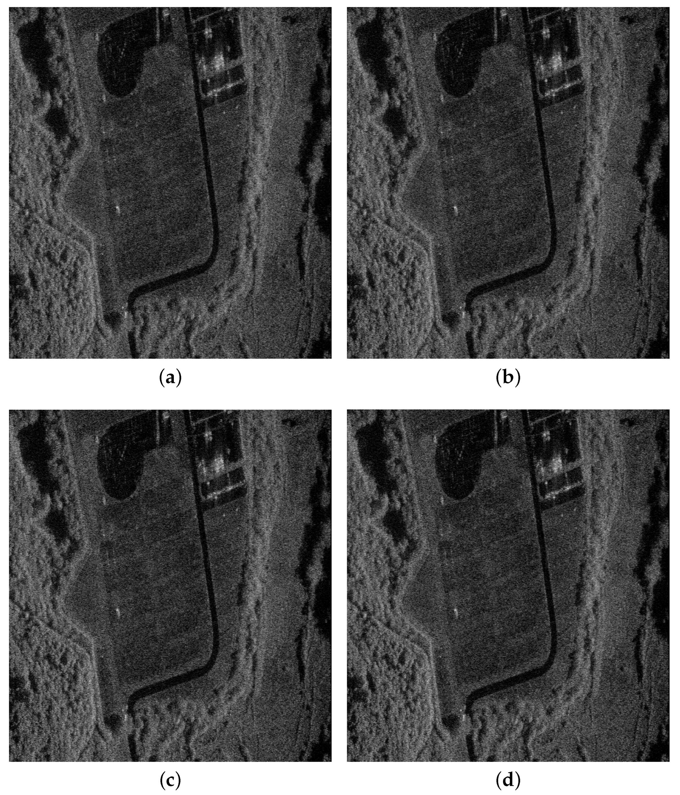
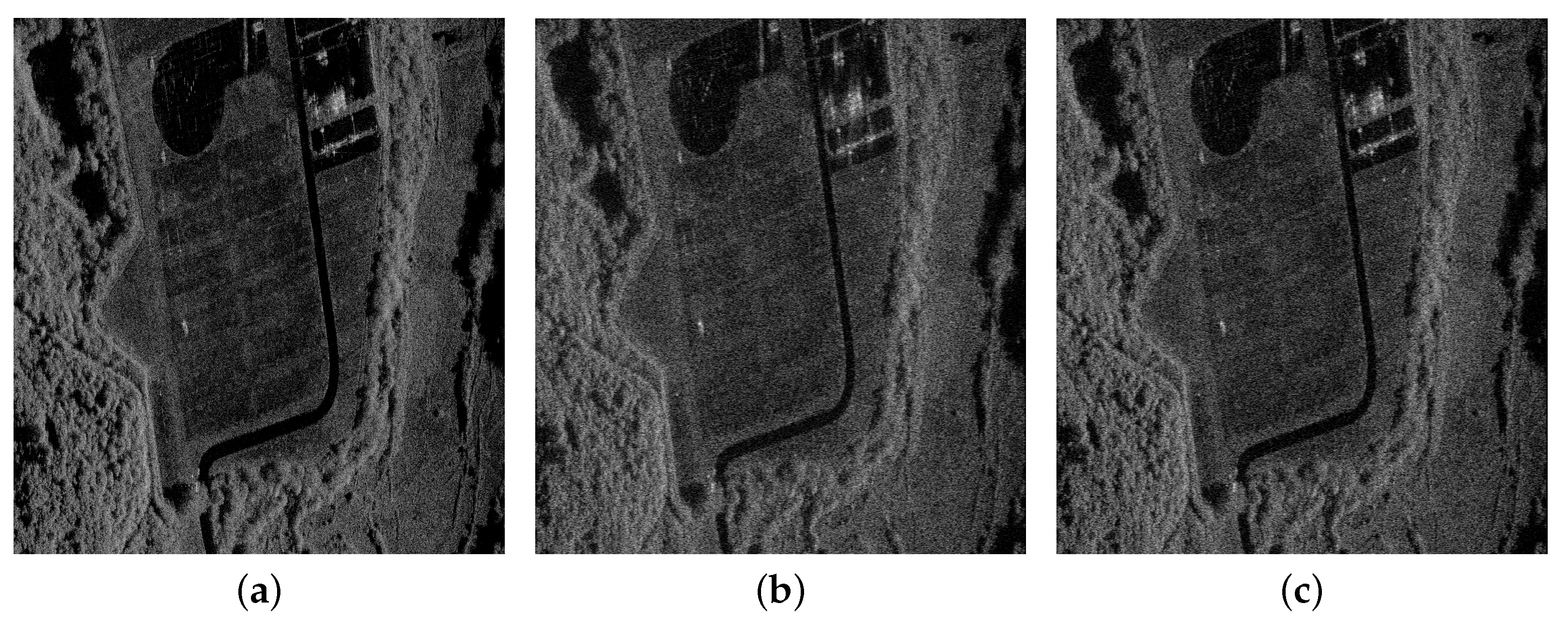
Figure 19.
Comparison of SAR images using different methods. (a) The empirically measured SAR image. (b) SAR image simulation based on the method of concentric circles. (c) SAR image generation based on time-domain simulation method.
Figure 19.
Comparison of SAR images using different methods. (a) The empirically measured SAR image. (b) SAR image simulation based on the method of concentric circles. (c) SAR image generation based on time-domain simulation method.
Figure 20.
Diagram depicting the results of the magnitude distribution comparison. (a) Concentric circles. (b) Time-domain simulation method.
Figure 20.
Diagram depicting the results of the magnitude distribution comparison. (a) Concentric circles. (b) Time-domain simulation method.
Figure 21.
The 3D model of the target.
Figure 21.
The 3D model of the target.
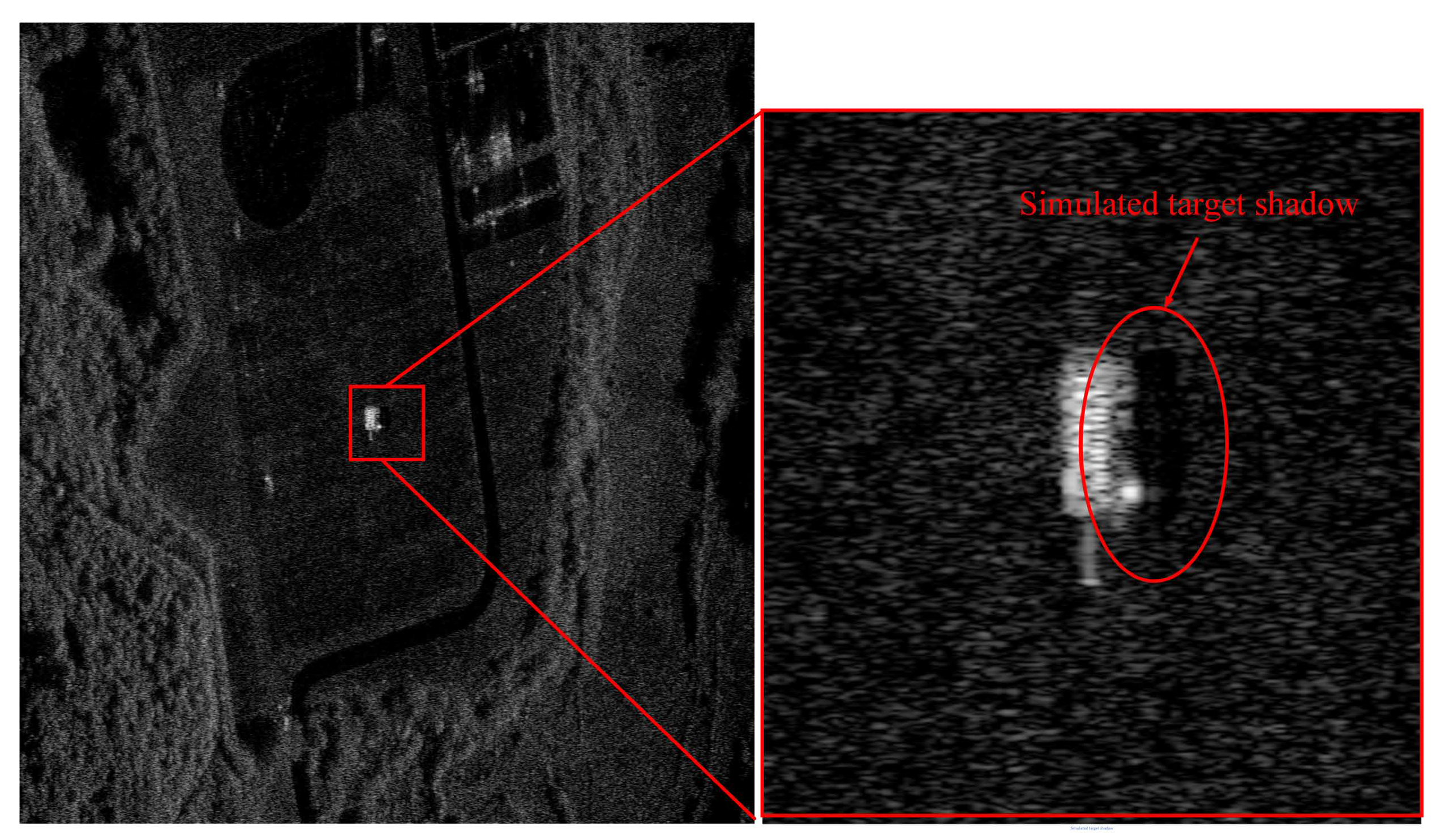
Figure 22.
SAR imaging with consideration of target shadows.
Figure 22.
SAR imaging with consideration of target shadows.
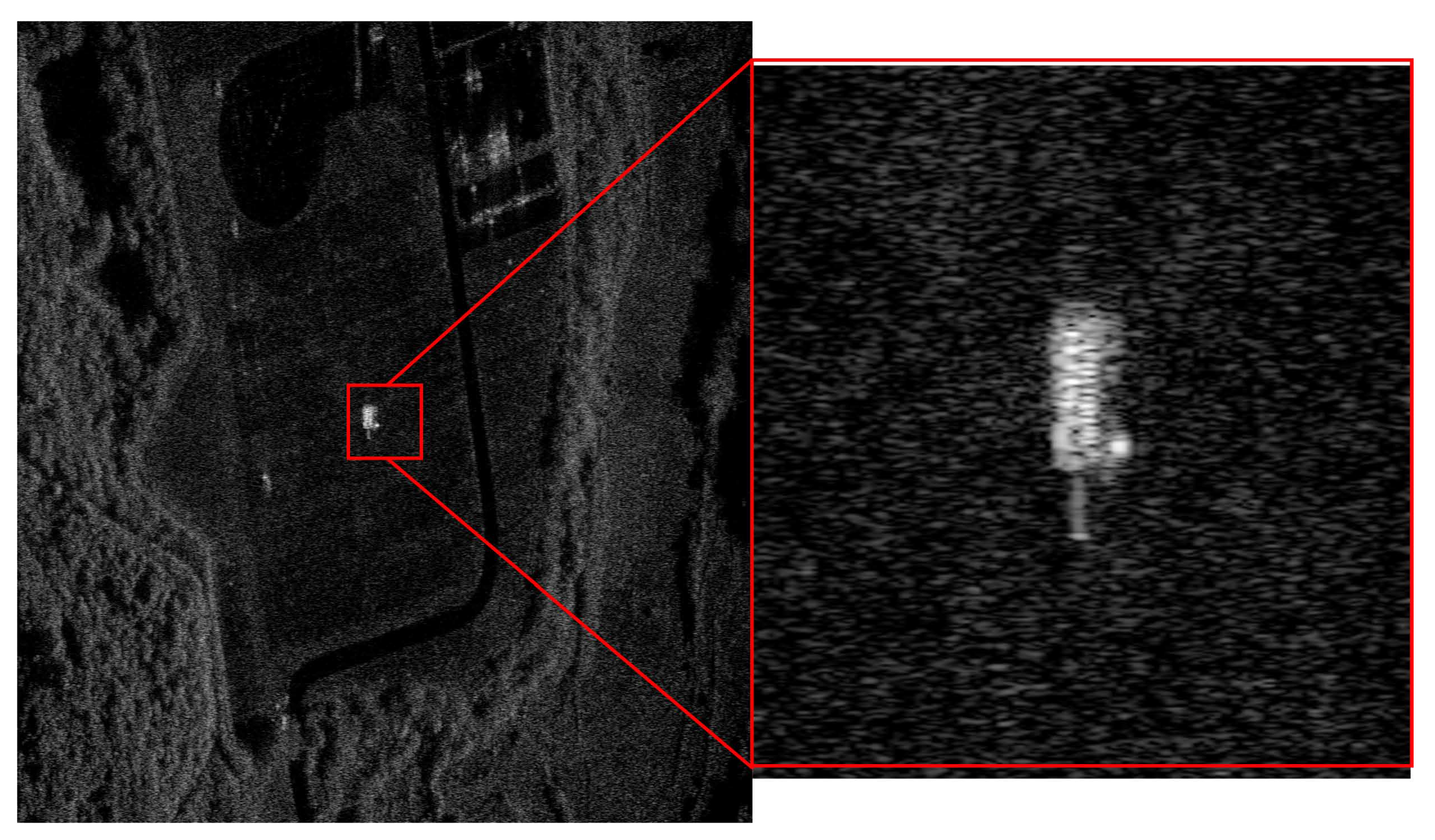
Figure 23.
SAR imaging without consideration of target shadows.
Figure 23.
SAR imaging without consideration of target shadows.
Table 1.
Simulation parameters.
Table 1.
Simulation parameters.
| Parameter | Value |
|---|
| Carrier frequency | 9.6 GHz |
| Signal pulse duration | 1 s |
| Sampling frequency | 591 MHz |
| Pulse repetition frequency | 1 KHz |
| Velocity | 150 m/s |
| Height | 1500 m |
| Elevation Angle | 15 |
| CPI | 2 s |
| Polarization | HH |
Table 2.
Comparison results of simulated images and MSTAR.
Table 2.
Comparison results of simulated images and MSTAR.
| | ZSU-234 | ZSU-234 | T62 | T62 |
|---|
| | | | | |
| | ([23]) | ([23]) | (Proposed) | (Proposed) |
| Similarity | 0.8093 | 0.8357 | 0.8989 | 0.8576 |
Table 3.
Measured SAR image parameters.
Table 3.
Measured SAR image parameters.
| Parameter | Value |
|---|
| Carrier frequency | 10 GHz |
| Scene size (Range × Azimuth) | 0.4 Km × 0.7 Km |
| The size of the flat terrain scene | 0.2 Km × 0.3 Km |
| The resolution in range domain | 0.25 m |
| The resolution in Azimuth domain | 0.125 m |
| Polarization | HV |
Table 4.
Simulation parameters.
Table 4.
Simulation parameters.
| Parameter | Value |
|---|
| Carrier frequency | 10 GHz |
| Signal bandwidth | 500 MHz |
| Signal pulse duration | 2 s |
| Pulse repetition frequency | 1 KHz |
| Beam angle | 20 |
| Velocity | 75 m/s |
| Height | 1500 m |
| Start of the flight path | (−1500,−150,1500) |
| End of the flight path | (−1500,150,1500) |
Table 5.
Cosine similarity of the magnitude distribution.
Table 5.
Cosine similarity of the magnitude distribution.
| | BW | BW | BW | BW |
|---|
| Similarity | 0.927 | 0.930 | 0.932 | 0.933 |
Table 6.
Runtime of concentric circles algorithm and traditional simulation algorithm.
Table 6.
Runtime of concentric circles algorithm and traditional simulation algorithm.
| | Concentric Circles | Time-Domain Simulation Method |
|---|
| time (s) | 340.744 | 28,876.527 |
Table 7.
Cosine similarity of the magnitude distribution.
Table 7.
Cosine similarity of the magnitude distribution.
| | Concentric Circles | Time-Domain Simulation Method |
|---|
| cosine similarity | 0.918 | 0.932 |


