Article

Comparison of Five Spectral Indices and Six Imagery Classification Techniques for Assessment of Crop Residue Cover Using Four Years of Landsat Imagery

Agricultural Research Service, Hydrology and Remote Sensing Laboratory, U.S. Department of Agriculture, Beltsville, MD 20705, USA
*
Author to whom correspondence should be addressed.
Remote Sens. 2023, 15(18), 4596; https://doi.org/10.3390/rs15184596
Submission received: 14 July 2023 / Revised: 1 September 2023 / Accepted: 14 September 2023 / Published: 19 September 2023
(This article belongs to the Special Issue Geographic Data Analysis and Modeling in Remote Sensing)

Abstract

:
Determining residue cover on agricultural land is an important task. Residue cover helps reduce soil erosion and helps sequester carbon. Many studies have used either spectral indices or classification techniques to map residue cover using satellite imagery. Unfortunately, most of these studies use only a few spectral indices or classification techniques and generally only study an area for a single year with a certain level of success. This manuscript presents an investigation of five spectral indices and six classification techniques over four years to determine if a single spectral index or classification technique performs consistently better than the others. A second objective is to determine whether using the coefficient of determination (R2) from the relationship between residue cover and a spectral index is a reasonable substitute for calculating accuracy. Field visits were conducted for each of the years studied and used to create the correlations with the spectral indices and as ground truth for the classification techniques. It was found that no spectral index/classification technique is consistently better than all the others. Classification techniques tended to be more accurate in 2011 and 2013, while spectral indices tended to be more accurate in 2015 and 2018. The combination of spectral indices/classification techniques outperformed the individual approach. For the second objective, it was found that R2 is not a great indicator of accuracy. Root mean square error (RMSE) is a better indicator of accuracy than R2. However, simply calculating the accuracy would be the best of all.

1. Introduction

Crop residue or senescent plant litter remaining on the surface of agricultural fields helps to reduce erosion, increase soil organic carbon, and protect soil health. The soil tillage intensity may be inferred from residue cover and is important regionally for government policies on soil carbon sequestration and water quality [1,2]. Soil health is important for maintaining farm sustainability [3].
Crop type and management (including tillage practices) may change each year. The Conservation Technology Information Center (CTIC) conducts roadside surveys for selected counties in the U.S. each year to measure and track the type of tillage used by crop at the county level. The accuracy of these surveys suffers from the low observation angle and the subjective nature of the observer [4,5].
Estimating residue cover on the soil surface with remote sensing has been studied, yet it is still challenging because soils and crop residues are spectrally similar at visible and near-infrared wavelengths [6]. However, dry crop residue has prominent absorption features in the shortwave infrared (SWIR) associated with lignin and cellulose [7,8,9]. There have been many attempts at developing spectral indices for the prediction of residue cover based on the cellulose absorption feature [3,10]. The Cellulose Absorption Index (CAI) developed by Daughtry [11] shows promise as an accurate index but requires relatively narrow spectral bands near 2020, 2110, and 2220 nm [12,13]. In contrast, multispectral satellite instruments, such as Landsat Thematic Mapper, provide only wide-band reflectance in the SWIR and do not allow direct measurement of the cellulose absorption feature.
Residue cover may also be estimated by land cover classification techniques using either multispectral [5,14] or hyperspectral sensors [15]. Many studies acquire hyperspectral imagery but analyze the data using spectral indices developed for multispectral sensors [16]. Some of the classification techniques originally developed for hyperspectral sensors, such as linear spectral unmixing and support vector machine, are just as applicable to the analysis of multispectral datasets. However, hyperspectral data have limited availability and relatively high cost; therefore, multispectral satellite sensors with a few broad spectral bands are currently the most likely to be used for operational assessment of cropland residue cover.
Most studies for assessing crop residue cover using multispectral imagery were conducted only for a single year, using spectral indices such as the Normalized Difference Index (NDI5,NDI7) [17], Simple Tillage Index (STI), Normalized Difference Tillage Index (NDTI) [18] and Normalized Difference Senescent Vegetation Index (NDSVI) [19]. These studies demonstrate the feasibility of new spectral indices or classification techniques but do not show the effects on accuracy of year-to-year variability in weather and farm operations, which is manifested as variation in the planting date and crop phenology. A few studies have been conducted over multiple years, but these studies generally focused on the feasibility of only a few spectral indices or classification techniques [2,20,21,22]. This study investigates the accuracy of multiple spectral indices as well as imagery classification techniques over multiple years.
In previous studies, a diversity of classification techniques have been used to assess the accuracy of spectral indices or classification results for predicting crop residue cover. Statistical methods, such as the coefficient of determination (R2) and root mean square error (RMSE), were used to assess the accuracy of continuous variables such as spectral indices. Categorical methods were used to handle classification analyses, summarized by an accuracy assessment matrix [23]. Accuracy is calculated by comparing the created classification with the observed values. The observed values can either come from the observations that were used to train the classification, or those that were set aside to validate the classification. Using the validation data is a more reasonable approach as the accuracy is not contaminated with the data used to create it. The prediction accuracies of spectral indices cannot be compared directly to prediction accuracies from classification. However, thresholds may be applied to the continuous spectral indices to obtain classification-like data, supporting a more direct comparison.
This study has two objectives. The first objective of this study is to compare the accuracy of five spectral indices and six imagery classifications over four years and to see if any are consistently superior to the others. The second objective is to determine the appropriateness of using R2 instead of accuracy when comparing spectral indices. We hypothesized for the first objective that while accuracies will change from year to year, the overall rank of each classification technique will be similar from year to year. For the second objective, we hypothesized that the use of R2 is not the best proxy for accuracy.

2. Materials and Methods

2.1. Study Area and Data Collection

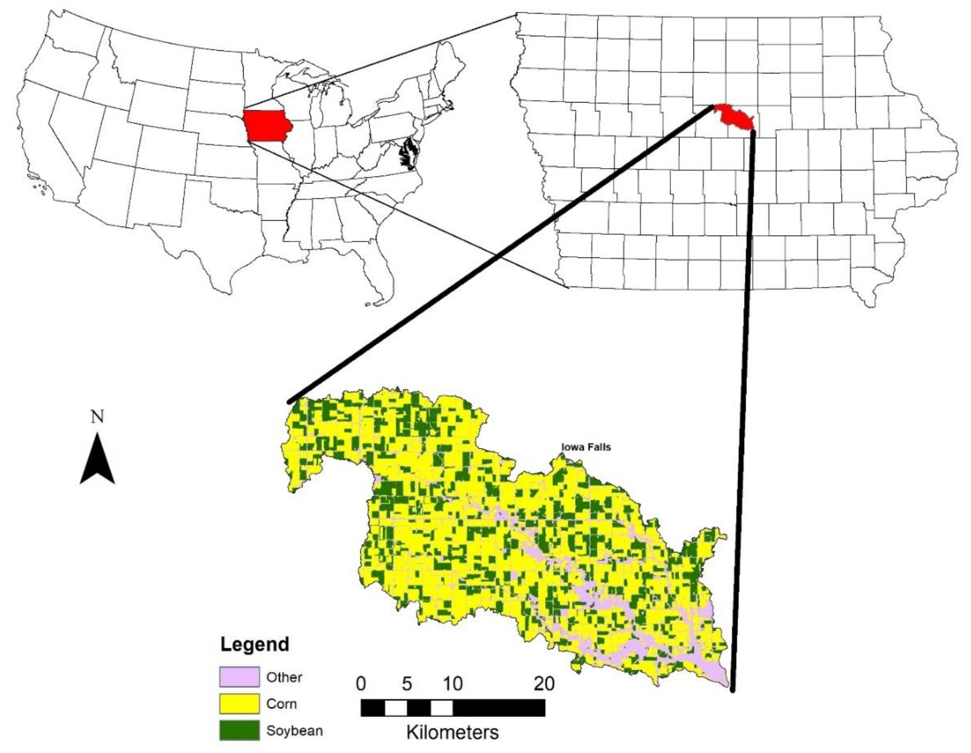
The study area was the South Fork of the Iowa River in Central Iowa. The watershed encompasses 810 km2. In 2010, the watershed was 56% corn and 25% soybean [24]. In 2017, the watershed remained roughly the same at 56% corn and 26% soybean [24]. A map showing the location of the watershed within Iowa and within the United States is shown in Figure 1.
The South Fork of the Iowa River is a Conservation Effects Assessment Project (CEAP) watershed. Some recent research involves assessing the effectiveness of conservation practices such as contour buffering and grassed waterways [25]. Other research focuses on modeling the subsurface drains, which assist in moving water from the surface of the field through the subsurface and into surface culverts [26].
Crop residue was measured in the spring of 2011, 2013, 2015, and 2018. Visits were timed so that corn planting was nearly completed (>90%) and soybean planting was >80%. The number of fields visited varied each year depending on which fields we had permission to visit and what tillage practices the farmer had implemented. Residue cover was measured from two locations per field that were at least 100 m from the edge of the field and at least 100 m from each other and relatively homogeneous. At each location a line-point transect of 15.2 m length was placed diagonally across the rows and residue was measured at 100 evenly spaced marks [4]. The line-point transect was then rotated 90 degrees and another measurement was taken. Thus, for each field there were four measurements (two at each location).

2.2. Remote Sensing Data and Methods

For each year, Landsat Imagery was acquired as near as possible to the date of the field data collection. Table 1 shows the type of Landsat sensors and the band width of each band. Since a sun photometer in Ames, IA approximately 60 km from the study site and atmospheric profiles were available from about 300 km away, MODTRAN [27] was used to convert each image to surface reflectance. The images were masked to remove pixels with substantial vegetation using the Normalized Difference Vegetation Index (NDVI) > 0.3 and to limit the analysis to pixels identified as planted with corn or soybean in the previous year using the Cropland Data Layer [24]. Since field sampling and associated imagery acquisition occurred in the springtime, the residue was left from the crop of the year before; thus, observations in the spring of 2011 identified residue from the summer crop of 2010.
Five spectral indices were calculated for each image:
Normalized Difference Index 5 (NDI5) = (NIR − SWIR1)/(NIR + SWIR1)
Normalized Difference Index 7 (NDI7) = (NIR − SWIR2)/(NIR + SWIR2)
Normalized Difference Tillage Index (NDTI) = (SWIR1 − SWIR2)/(SWIR1+SWIR2)
Simple Tillage Index (STI) = SWIR1/SWIR2
Normalized Difference Senescent Vegetation Index (NDSVI) = (SWIR1 − Red)/(SWIR1 + Red)
These spectral indices have been used frequently in previous studies [17,18,19]. In addition, six imagery classification techniques were tested. These classification techniques have been found in various papers for classifying residue levels and are readily available from software packages [2,14,28,29,30]. In this study, ENVI/IDL was used for Mahalanobis Distance, Minimum Distance, and Spectral Angle Mapper; ARCGIS was used for Maximum Likelihood, Random Tree, and Support Vector Machine; and in all cases, the default parameters were used. For each year of data, a multiband image was created using the Landsat bands listed in Table 1. The basis for classifying crop residue cover using Landsat is that dry crop residue shows different spectral reflectance, especially in the SWIR bands in which residue cover has significant absorption features different from the soil.
The following classification techniques were applied:
  • Minimum Distance (MINDIST) assigns the class based on the class with the smallest Euclidean distance in n-space from the unclassified pixel to the mean of the known class [31].
  • Maximum Likelihood (MAXLI) assigns the unclassified pixel to the class which is most probably a part of assuming each class in each band is normally distributed [31].
  • Mahalanobis distance (MAHLDIST) is similar to maximum likelihood but assumes all class covariances are equal [31].
  • Random tree (RANDTR) classified unclassified pixels based on a series of decisions which lead to the known classes [32].
  • Spectral Angle Mapper (SAM) creates a modified spectra from the training data, based on the angle between the various bands. It assigns each unclassified pixel to the spectra that it matches the best [33].
  • Support Vector Machine (SVM) uses a decision surface or optimal hyperplane that maximizes the difference between the classes [34].
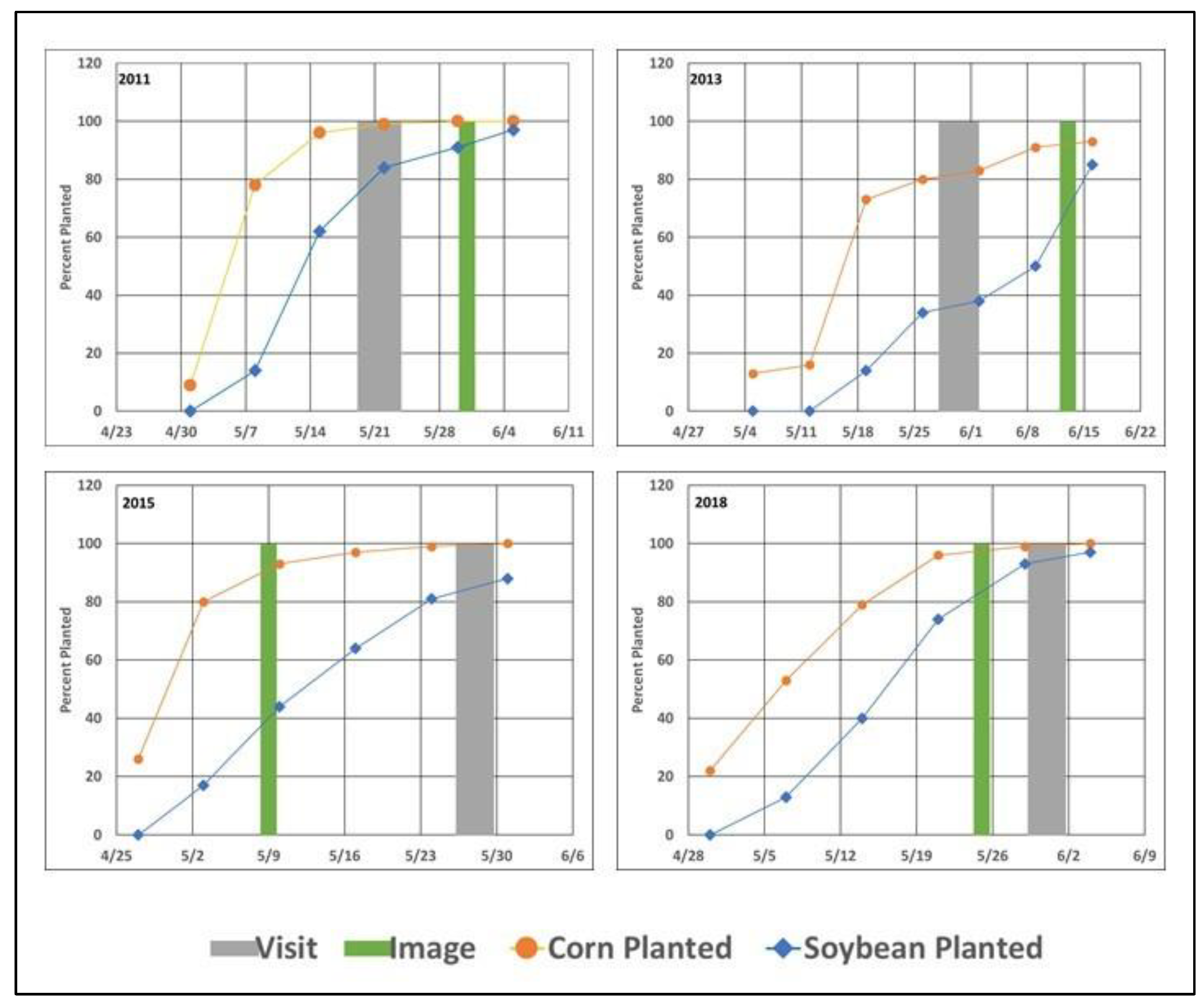
Table 2 shows the date of the image used and the date of the field visit. Figure 2 shows the timing of the field visits relative to imagery acquisition and the crop status [35]. In two cases, the field sampling occurred prior to image acquisition, and in two cases, it occurred after imagery acquisition. The longest separation (18 days) was in 2015. For field visits that occurred prior to imagery acquisition, nearly all fields had been tilled. For field visits that occurred after imagery acquisition, it is impossible to know how much field activity took place between the image and the field visit.

2.3. Data Preparation

Crop residue measurements for each field were averaged and the residue type (corn, soybean) was assigned based on the previous year’s crop. The fields were placed into a class based on the amount of observed residue according to CTIC [36] guidelines: intensive tillage (less than 15% residue), reduced tillage (15–30% residue) and conservation tillage (greater than 30% residue). Conservation tillage was then split into two classes (30–60% residue and greater than 60% residue), for a total of four classes (Table 3).
For each class, approximately 2/3 of the fields (stratified for even representation of each class type) were used to calculate the correlation between residue cover and spectral indices and were also used as training data for the classification techniques (Training). The remaining 1/3 of the data was used to test the accuracy of the classifications (Validation). Table 3 shows the total number of fields in each residue category and the number used for training and for validation.
To derive a classified image of fractional residue cover, the average observed percentage of residue cover for each training field was linearly correlated with the average spectral index values for each field to derive a relationship between residue cover and the spectral indices. The resulting equations were then applied to the imagery-derived raster maps of spectral index values to create an image of predicted residue cover on corn and soybean fields, which was then assigned to one of the four levels of crop residue cover.
To derive input for the six classification techniques, each sampled training field was assigned to a residue grouping based on the average observed crop residue cover. The mean and standard deviation (SD) of reflectance for each multispectral band was then derived for each training field and was used in the classification process. The resulting classified residue image consisted of the four levels of residue cover (0–15, 15–30, 30–60, 60–100%).
Lastly, to see the impact of combining both classification techniques and spectral indices, two different procedures were performed. In the first, the most frequent class of all classification techniques and spectral indices was selected as the class for each pixel; for simplicity, this will be referred to as ALL. In the second, the most frequent class of STI, NDI7, SVMC, and RANDTR was selected as the class for each pixel; for simplicity, this will be referred to as FOUR.

2.4. Accuracy Assessment

For the first objective (determining if a single classification or spectral index is the most accurate), accuracy was assessed by using the thematic crop residue image ((number of pixels correctly classified / number of total pixels) × 100%). In this case, while we assume the validation field is uniform, we compare the field average of in situ measurements to the pixels that make up the field from the thematic crop residue image.
For the second objective (determining if using Training R2 is a reasonable proxy for validation accuracy), the numeric residue image is created by applying each correlation equation to the index. The residue is averaged for each field and then each field is placed in one of the four levels. To calculate the accuracy, each averaged field is compared to the observed residue values ((number of fields correctly classified/number of total fields) × 100%). In addition to R2, root mean square error (RMSE) was calculated based on the average field information.
In addition to accuracy, it is important to look at Kappa and Z. Kappa is an indication of how much better than chance the observed distribution of points is. Kappa is defined as:
Kappa = (po − pe)/(1 − pe)
where po is the relative observed agreement among classes and pe is the hypothetical probability of chance agreement. If Kappa is zero, then the distribution is no better than chance, Kappa’s top value is 1. Z is a measure of how statistically significant the Kappa value is. Z is defined as:
Z = (X − E[X})/SD(X)
where X is the variable and E[X} is the expected value divided by the standard deviation. While accuracy is commonly used to determine how well a classification or index has worked, Kappa and Z are also important indicators of classification performance.
The accuracy for each spectral index and classification technique was calculated for each year using the validation data set. The average and standard deviation of the accuracies were calculated for the four years. The four-year averages were then sorted from most accurate to least accurate. In addition, the average and standard deviation of all the index/methods were calculated for each year.

3. Results and Discussion

3.1. Results from Discussion

The results are shown in Table 4, with values that are more than one standard deviation above the mean in blue and those more than one standard deviation below the mean in red. Similar processes were also carried out for Kappa and Z, as shown later in this section.
The least accurate year for the measurement of residue cover was 2013 with an accuracy of 45.79%. However, the best year, 2011, at 56.51%, was only 11% higher. This points to the difficulty of measuring residue cover using broadband spectral data. In 2011, classification techniques were more accurate than spectral indices, and this was partially true in 2013. In 2015 and 2018, spectral indices were more accurate than classification techniques. Of the classification techniques, SVMC and RANDTR were the most accurate and MINDIST and SAM were the least accurate. Overall, the spectral indices produced similar results, with four-year average accuracies ranging from 52.42 to 55.60%. STI, NDTI and MAXLI have at least one year where they are more than one standard deviation above the mean and at least one standard deviation below the mean. This shows that just because on a given year a spectral index or classification technique does well (badly), on a different year, they will perform the same.
It is interesting to note that classification techniques were more accurate than spectral indices in years when the field visit preceded the image, while spectral indices were more accurate than classification techniques in years in which the image preceded the field visit. It is speculated that spectral indices are more resistant to changes in the residue levels between image and visit times. It is preferable/ideal to have both field visits and imagery shortly after most field activities have been completed. However, satellite revisit schedules and weather (cloud and rain) interfere with the ability to obtain images at the ideal time. In cases in which the image is after the visit, most field activities have finished, and there is no change in residue cover, which classification techniques perform well with. If the image preceded the field visit, it is possible field activities were still going on, changing the residue cover between the image and field visit, which are the circumstances that spectral indices perform better in.
The combination of ALL and FOUR performed very well. FOUR was more accurate than any of the individual spectral indices or classification techniques, ranking most accurate in 2011, 2013, 2015 and second highest in 2018. ALL performed slightly worse, ranking first in 2013, third in 2011 and 2015 and fourth in 2018. It should be noted that ALL and FOUR were ranked in comparison to the individual spectral indices/classification techniques and not to each other, hence both being ranked first in 2013.
To understand the importance of calculating Kappa and Z, Table 5 shows results using data from 2013. In the example from 2013, NDI5 has an overall accuracy of 49.01%, but everything has been classified as class 3, which is not very meaningful. In comparison, NDTI has an accuracy of 39.25%, but the points are distributed more meaningfully, and the Kappa and Z are higher as a result. This shows the importance of using Kappa and Z in addition to accuracy. It is possible to have an accuracy near 50% simply by chance.
Table 6 and Table 7 show Kappa and Z values for classification techniques and spectral indices associated with overall rank. Kappa and Z mimic each other and, similar to the accuracies (Table 4), 2013 showed the worst performance. Like the accuracies, except for MINDIST, which was consistently bad, classification techniques performed better than spectral indices in 2011 and 2013 and spectral indices performed better in 2015 and 2018. For the classification techniques, the similarity with accuracy continued with SVMC performing the best and SAM and MINDIST performing the worst. The spectral index results departed from the pattern in accuracies. STI and NDTI performed the best, and NDI5 performed the worst.
FOUR is ranked highest for Kappa in 2011, 2015, and 2018 and second in 2013. ALL performed slightly worse. Only in Z does FOUR perform slightly worse, ranking second in 2011, third in 2015, and fourth in 2013 and 2018. ALL also shows a similar reduction in rank. It should be noted that because certain pixels do not have a most-frequent class, some pixels were lost in the combination process. ALL contained between 92.7 and 97.4% of the individual spectral indices/classification techniques. FOUR contained between 67.3 and 74.2% of the pixels. The reduction in pixels is probably shown in the rank decrease in Z, even though the accuracy and Kappa rated higher.
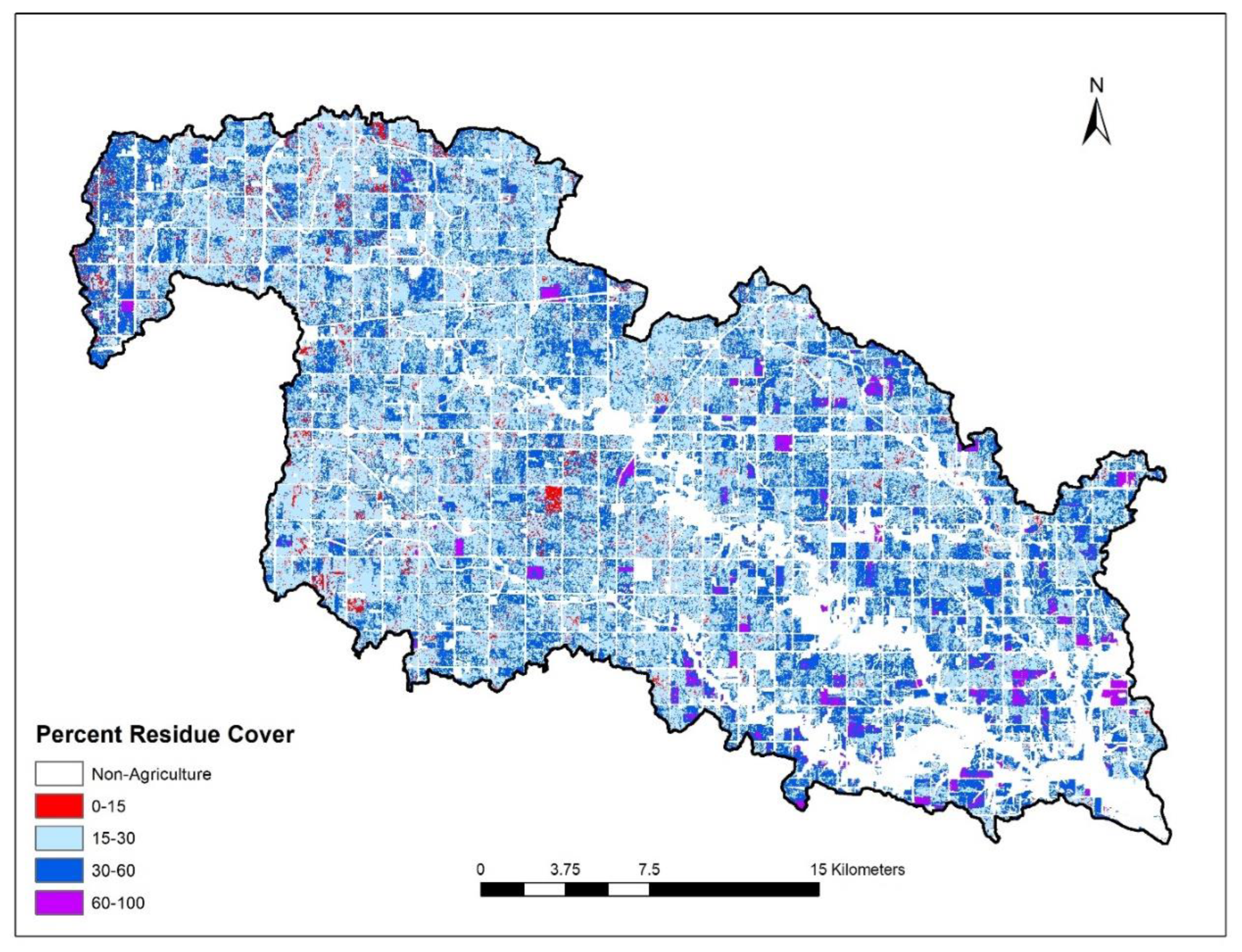
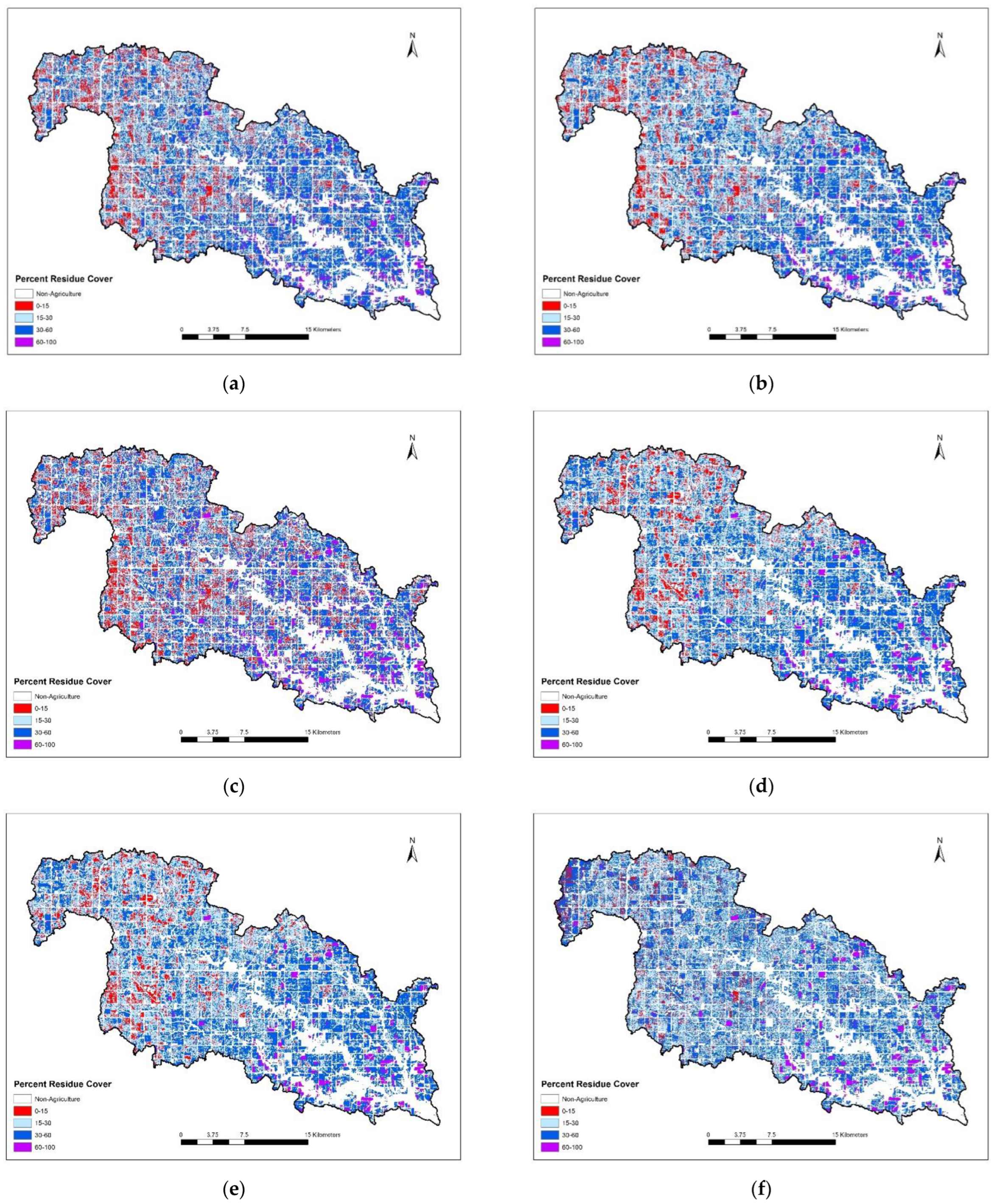
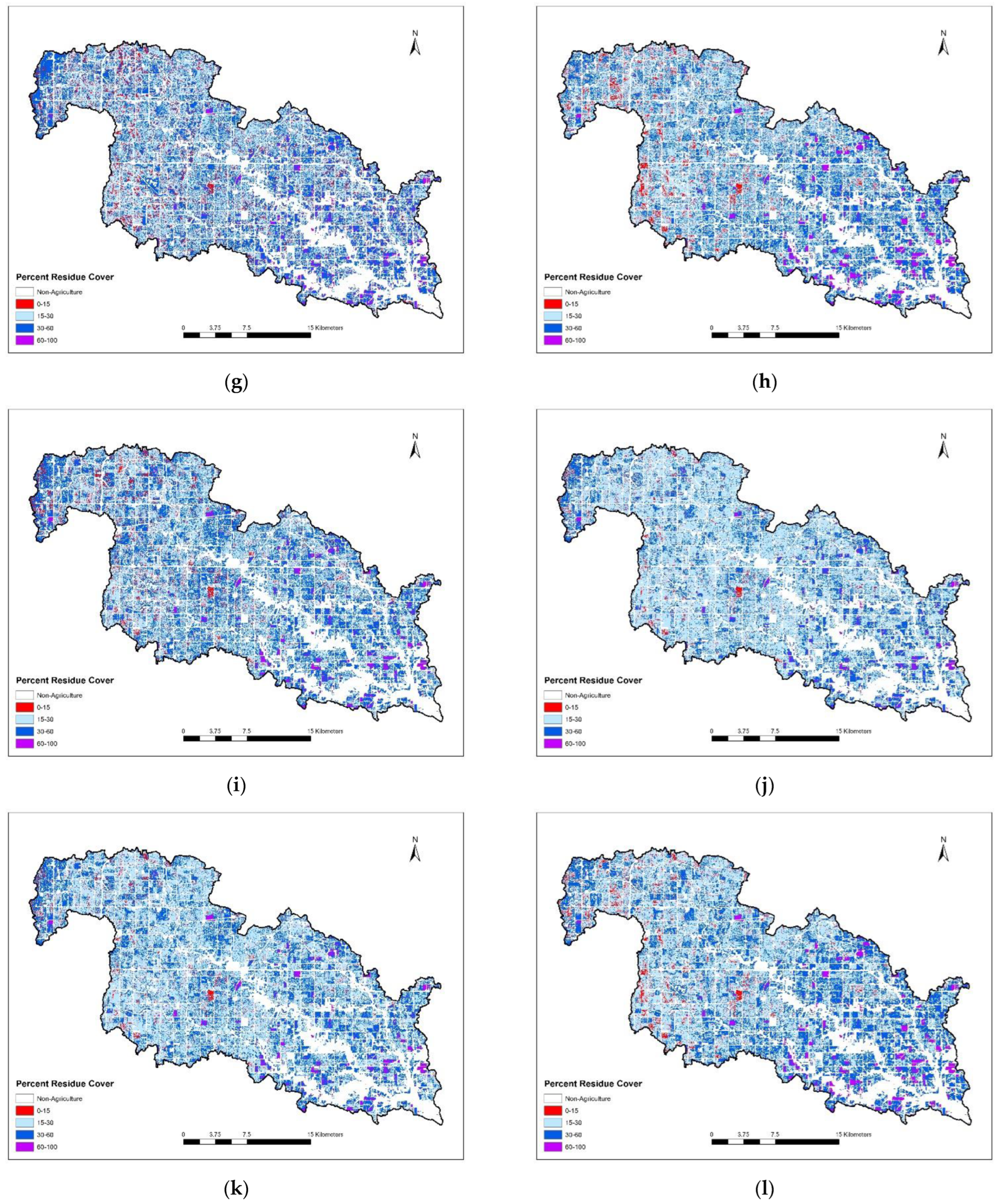
Figure 3 demonstrates a residue map created by using SVMC for 2011. Except for the very western edge of the watershed, there is a general increase in no-till toward the east (the mouth of the watershed), as the terrain becomes steeper. Figure A1 in Appendix A show the residue cover maps of all spectral indices/classification techniques and the two combinations for 2011.

3.2. Appropriateness of Using Training R2 As a Surrogate for Validation Accuracy

To analyze the appropriateness of using R2 from training data as a surrogate for validation accuracy, the field-based R2 from training data were used. However, unlike the previous objective, the resulting residue image was averaged at the field level before being grouped into the four levels of residue. R2 and RMSE were calculated from the numeric average residue for each field, while accuracy, Kappa and Z were calculated based on the thematic level of residue cover (0–15, 15–30, 30–60, 60–100).
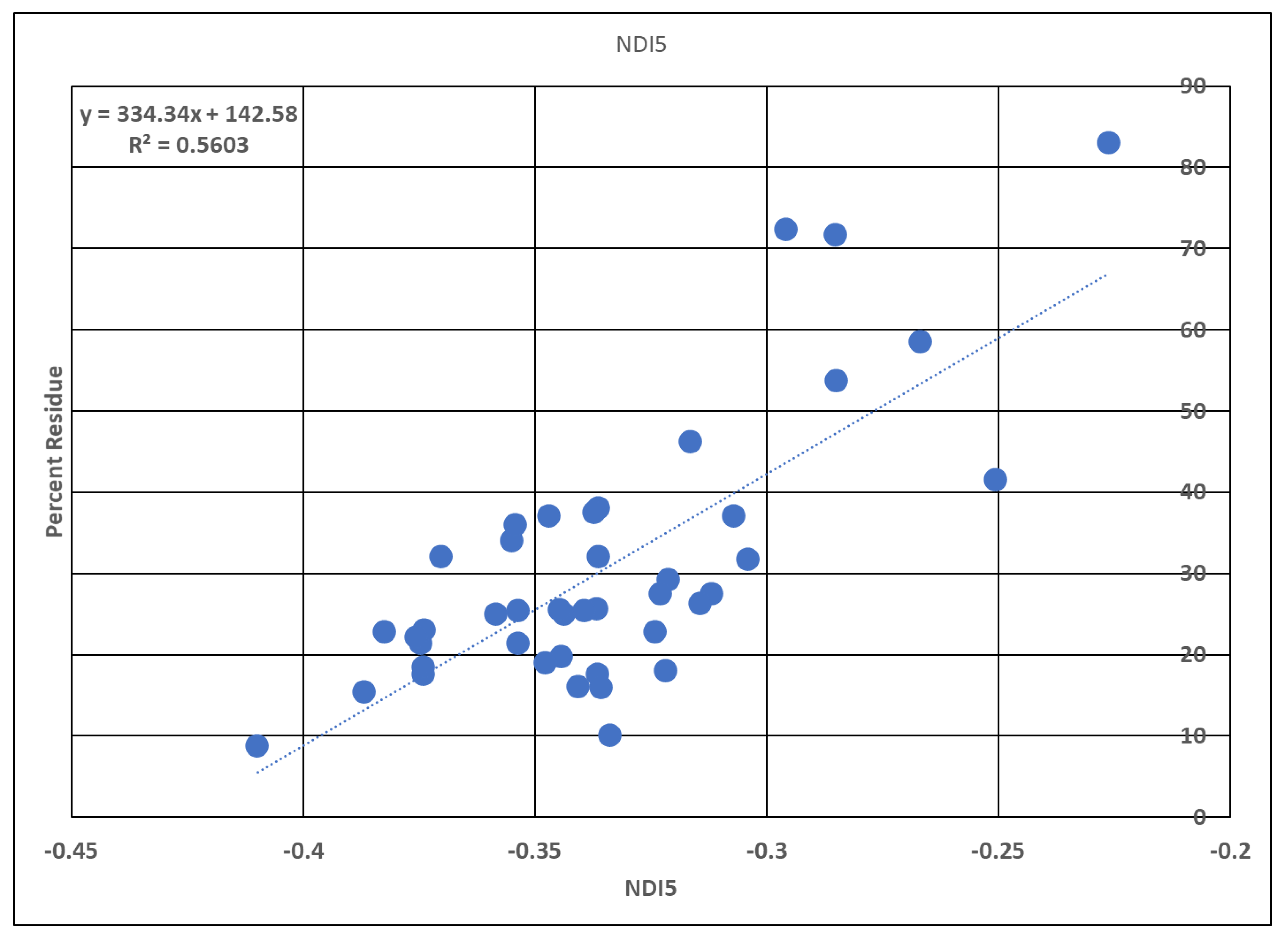
The process of calculating R2 for the various spectral indices was conducted in several steps. To understand the process, NDI5 in 2011 will be used as an example. The training data in 2011 consisted of 43 fields. First, NDI5 and the sample residue data were averaged at the field level. Figure 4 shows the results, with an R2 of 0.5603. Second, the reference data and the created residue map were grouped into four groups (0–15, 15–30, 30–60, 60–100) and compared. Table 8 shows the accuracy matrix and the results of the overall accuracy of 55.81%, Kappa of 0.227 and Z of 1.72. Third, the process was repeated for each year and each spectral index each created their own; see Figure 4 and Table 8.
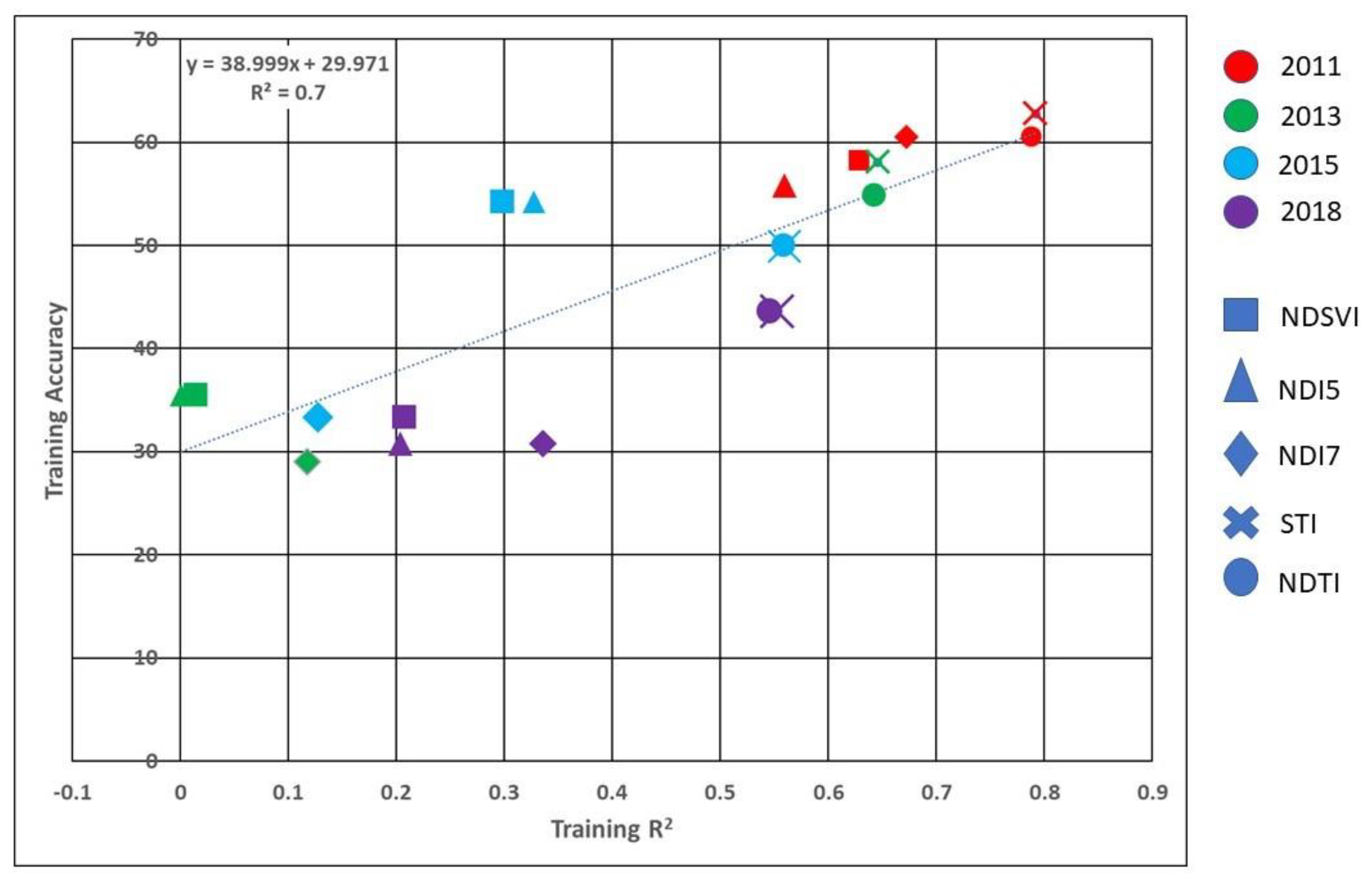
Figure 5 shows the result of R2 and accuracy from training samples for five spectral indices and four years (20 points). The R2 of the 20 points in Figure 5 was computed (0.7). The red triangle at training R2 of 0.5603 and training accuracy of 55.81% is the example. Finally, Table 9 summarizes the R2 of each combination tested with the R2 from the example being on the first row (i.e., Training R2 vs. Training Accuracy).
Table 9 shows that the R2 varies when using different metrics to assess accuracy. Among combinations, the training data RMSE and training data accuracy have the highest R2 of 0.758. While the training data R2 shows a good correlation, it still would be best to simply calculate the accuracy. It should be noted that comparing training data R2 and the accuracy from the validation data results in an R2 of 0.528, which means training data R2 is not a bad indicator of performance. However, the validation R2 is poorly correlated to training accuracy (0.025) and validation accuracy (0.024). Like the training data, R2 is slightly higher at 0.584 when comparing training data accuracy and the validation RMSE. The training accuracy and validation accuracy are not well correlated (R2 = 0.237), which implies that the training accuracy may not be a good indicator of the validation accuracy. Validation samples must be reserved during experiment design for accuracy assessment.

3.3. Limitations

This study is based on the South Fork of the Iowa River situated in Central Iowa. The outcomes generated from this investigation are anticipated to have broad applicability across a significant portion of the corn belt region. However, it is essential to acknowledge that these findings might not directly translate to areas with diverse crops, soils, climates, and weather patterns.
The collection of field data was conducted over a span of four years (2011, 2013, 2015, and 2018). Although this timeframe offers insights, it is important to note that it does not encompass the full spectrum of potential weather variations and soil moisture levels. Thus, there is a need for further research to capture a more complete understanding.
The paper investigates five spectral indices and six classification techniques that are commonly used for crop residue cover mapping. It is worth noting that more advanced techniques may yield even more accurate results. It is expected that new satellite missions with more frequent observations (e.g., Sentinel-2) or additional narrow shortwave infrared reflectance bands (e.g., Landsat Next or Landsat 10) can provide a more accurate result in crop residue mapping.
4. Conclusions

Residue cover can be estimated by remote sensing spectral indices and classification techniques. In general, spectral indices have better accuracies than classification techniques. This is probably because the relationship between index and residue is more tolerant of fields that do not closely match the relationship. However, as seen in the 2011 result, this is not always true. We found that the timing between observation and imagery also plays an important role in residue cover mapping. By combining STI, NDI7, SVMC and RANDTR (FOUR combination), it was possible to create a residue class image that was more accurate than any spectral indices/classification technique alone. Combining all spectral indices/classification techniques also produced good results, but the results were generally worse than the FOUR combination.
The secondary study shows the limitation of using R2 as an indicator to assess the performance of an index. R2 is not a great indicator of accuracy, and additional evaluation metrics are needed in the accuracy assessment.
Lastly, using training and testing data is important. Without validation, data accuracies will be inflated. In particular, the correlation of training data and validation data accuracies for the field spectral indices was particularly low.
This study shows that crop residue cover and soil tillage intensity can be mapped at a reasonable accuracy with the selected index and classification techniques. Landsat imagery provides a way to map crop residue cover at a large scale to support agroecosystem monitoring.

Author Contributions

Conceptualization, methodology, software, validation, formal analysis, investigation, data curation, writing—original draft preparation, A.J.S.; writing—review and editing, A.J.S., C.S.T.D., E.R.H.J. and F.G. All authors have read and agreed to the published version of the manuscript.

Funding

This research received no external funding.

Data Availability Statement

The data presented in this study are available on request from the corresponding author. The data are not publicly available due to confidentiality.

Acknowledgments

The research was a contribution from the Long-Term Agroecosystem Research (LTAR) network. LTAR is supported by the United States Department of Agriculture. USDA is an equal opportunity provider and employer. Any use of trade, firm or product names is for descriptive purposes only and does not imply endorsement by the U.S. Government.

Conflicts of Interest

The authors declare no conflict of interest.

Appendix A

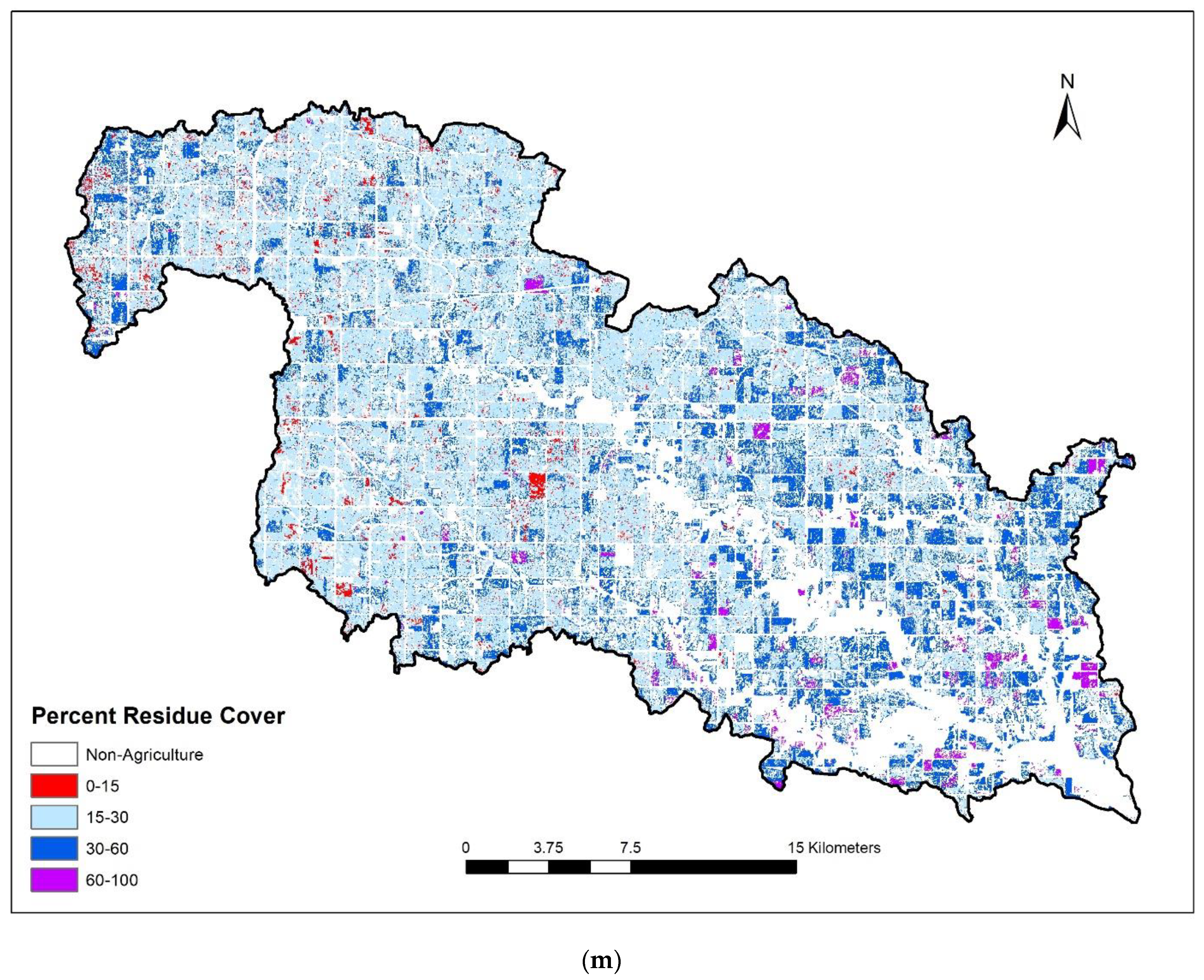
Figure A1. Results for spectral indices/classification techniques for 2011. (a) NDI5, (b) NDI7, (c) NDSVI, (d) NDTI, (e) STI, (f) MAHL, (g) MINDIST, (h) SAM, (i) MAXLI, (j) RANDTR, (k) SVMC, (l) ALL, (m) FOUR.
Remotesensing 15 04596 g0a1aRemotesensing 15 04596 g0a1bRemotesensing 15 04596 g0a1c

References

  1. Daughtry, C.S.T.; Doraiswamy, P.C.; Hunt, E.R., Jr.; Stern, A.J.; McMurtrey, J.E., III; Prueger, J.H. Remote sensing of crop residue cover and soil tillage intensity. Soil Tillage Res. 2006, 91, 101–108. [Google Scholar] [CrossRef]
  2. Beeson, P.C.; Daughtry, C.S.T.; Hunt, E.R.; Akhmedov, B.; Sadeghi, A.; Karlen, D.L.; Tomer, M.D. Multispectral satellite mapping of crop residue cover and tillage intensity in Iowa. J. Soil Water Conserv. 2016, 71, 385–395. [Google Scholar] [CrossRef]
  3. Zheng, B.; Campbell, J.B.; Serbin, G.; Galbraith, J.M. Remote sensing of crop residue and tillage practices: Present capabilities and future prospects. Soil Tillage Res. 2014, 138, 26–34. [Google Scholar] [CrossRef]
  4. Morrison, J.E., Jr.; Huang, C.; Lightle, D.T.; Daughtry, C.S.T. Residue cover measurement techniques. J. Soil Water Conserv. 1993, 48, 479–483. [Google Scholar]
  5. Thoma, D.P.; Gupta, S.C.; Bauer, M.E. Evaluation of optical remote sensing models for crop residue cover assessment. J. Soil Water Conserv. 2004, 59, 224–233. [Google Scholar]
  6. Aase, J.K.; Tanaka, D.L. Reflectance from four wheat residue cover densities as influenced by three soil backgrounds. Agron. J. 1991, 83, 753–757. [Google Scholar] [CrossRef]
  7. Elvidge, C.D. Visible and near infrared reflectance characteristics of dry plant materials. Remote Sens. 1990, 11, 1775–1795. [Google Scholar] [CrossRef]
  8. Kokaly, R.F.; Asner, G.P.; Olinger, S.V.; Martin, M.E.; Wessman, C.A. Characterizing canopy biochemistry from imaging spectroscopy and its application to ecosystem studies. Remote Sens. Environ. 2009, 113, S78–S91. [Google Scholar] [CrossRef]
  9. Daughtry, C.S.T.; Hunt, E.R.; McMurtrey, J.E. Assessing crop residue cover using shortwave infrared reflectance. Remote Sens. Environ. 2004, 90, 126–134. [Google Scholar] [CrossRef]
  10. Bannari, A.; Pacheco, A.; Staenz, K.; McNairn, H.; Omari, K. Estimating and mapping crop residues cover on agricultural lands using hyperspectral and IKONOS data. Remote Sens. Environ. 2006, 104, 447–459. [Google Scholar] [CrossRef]
  11. Daughtry, C.S. Discriminating crop residues from soil by shortwave infrared reflectance. Agron. J. 2001, 93, 125–131. [Google Scholar] [CrossRef]
  12. Hively, W.D.; Lamb, B.T.; Daughtry, C.S.T.; Serbin, G.; Dennison, P.; Kokaly, R.F.; Wu, Z.; Masek, J.G. Evaluation of SWIR Crop Residue Bands for the Landsat Next Mission. Remote Sens. 2021, 13, 3718. [Google Scholar] [CrossRef]
  13. Nagler, P.L.; Daughtry, C.S.T.; Goward, S.N. Plant litter and soil reflectance. Remote Sens. Environ. 2000, 71, 207–215. [Google Scholar] [CrossRef]
  14. South, S.; Qi, J.; Lusch, D.P. Optimal classification methods for mapping agricultural tillage practices. Remote Sens. Environ. 2004, 91, 90–97. [Google Scholar] [CrossRef]
  15. Chi, J.; Crawford, M.M. Spectral unmixing-based crop residue estimation using hyperspectral remote sensing data: A case study at purdue university. IEEE J. Sel. Top. Appl. Earth Obs. Remote Sens. 2014, 7, 2531–2539. [Google Scholar] [CrossRef]
  16. Daughtry, C.S.T.; Hunt, E.R.; Doraiswamy, P.C.; McMurtrey, J.E. Remote sensing the spatial distribution of crop residues. Agron. J. 2005, 97, 864–871. [Google Scholar] [CrossRef]
  17. McNairn, H.; Protz, R. Mapping corn residue cover on agricultural fields in Oxford County, Ontario, using Thematic Mapper. Can. J. Remote Sens. 1993, 19, 152–159. [Google Scholar] [CrossRef]
  18. VanDeventer, A.P.; Ward, A.D.; Gowda, P.H.; Lyon, J.G. Using Thematic Mapper data to identify contrasting soil plains and tillage practices. Photogram. Eng. Remote Sens. 1997, 63, 87–93. [Google Scholar]
  19. Qi, J.; Marsett, R.; Hellman, P.; Biedenbender, S.; Moran, M.S.; Goodrich, D.C.; Weltz, M. RANGES improves satellite-based information and land cover assessments in Southwest United States. EOS Trans Am. Geophys. Union 2002, 83, 601–606. [Google Scholar] [CrossRef]
  20. Sonmez, N.K.; Slater, B. Measuring Intensity of Tillage and Plant Residue Cover using Remote Sensing. Eur. J. Remote Sens. 2016, 49, 121–135. [Google Scholar] [CrossRef]
  21. Rossi, F.S.; DaSilva, C.A., Jr.; de Oliverra, J.F., Jr.; Teodoro, P.E.; Shiratruchi, L.S.; Lima, M.; Teodoro, L.P.R.; Tiago, A.V.; Capristo-Silva, G.F. Identification of tillage for Soybean crop by Spectro-temporal variables GEOBIA and decision tree. Remote Sens. Appl. Soc. Environ. 2020, 19, 100356. [Google Scholar] [CrossRef]
  22. Watts, J.D.; Lawrence, R.L.; Miller, P.R.; Montagne, C. Monitoring of Cropland Practices for carbon sequestration purposes in north central Montana by Landsat remote sensing. Remote Sens. Environ. 2009, 113, 1843–1852. [Google Scholar] [CrossRef]
  23. Congalton, R.G.; Green, K. Assessing the Accuracy of Remotely Sensed Data: Principles and Practices; CRC Press: Boca Raton, FL, USA, 2019. [Google Scholar]
  24. USDA National Agricultural Statistics Service, Cropland Data Layer 2010, 2012, 2014, 2017, Published Crop Specific Data Layer. Available online: https://croplandcros.scinet.usda.gov (accessed on 11 July 2023).
  25. Moorman, T.B.; James, D.E.; Van Horn, J.; Porter, S.A.; Tomer, M.D. Temporal trends in amount and placement of conservation practices in the South Fork of the Iowa River Watershed. J. Soil Water Conserv. 2020, 75, 245–253. [Google Scholar] [CrossRef]
  26. Bailey, R.T.; Bieger, K.; Flores, L.; Tomer, M. Evaluating the contribution of subsurface drainage to watershed water yield SWAT+ with groundwater modeling. Sci. Total Environ. 2022, 802, 149962. [Google Scholar] [CrossRef] [PubMed]
  27. Berk, A.; Anderson, G.P.; Acharya, P.K.; Bernstein, L.S.; Muratov, L.; Lee, J.; Fox, M.J.; Adler-Golden, S.M.; Chetwynd, J.H.; Hoke, M.L.; et al. Modtran 5: A reformulated atmospheric band model with anxilary species and practical multiple scattering options. In Proceedings of the Fourth International Asia-Pacific Environmental Remote Sensing Symposium: Remote Sensing of the Atmosphere, Ocean, Environment and Space, Honolulu, HI, USA, 8–12 November 2004; Volume 5655, pp. 88–95. [Google Scholar]
  28. Castillejo-González, I.L.; López-Granados, F.; García-Ferrer, A.; Peña-Barragán, J.M.; Jurado-Expósito, M.; Sánchez de la Orden, M.; González-Audicana, M. Object- and pixel-based analysis for mapping crops and their agro-environmental associated measures using QuickBird imagery. Comput. Electron. Agric. 2009, 68, 207–215. [Google Scholar] [CrossRef]
  29. Zhu, Q.; Xu, X.; Sun, Z.; Liang, D.; An, X.; Chen, L.; Yang, G.; Huang, L.; Xu, S.; Yang, M. Estimation of Winter Wheat Residue Coverage Based on GF-1 Imagery and Machine Learning Algorithm. Agronomy 2022, 12, 1051. [Google Scholar] [CrossRef]
  30. Riegler-Nurscher, P.; Prankl, J.; Bauer, T.; Strauss, P.; Prankl, H. A machine learning approach for pixel wise classification of residue and vegetation cover under field conditions. Biosyst. Eng. 2018, 169, 188–198. [Google Scholar] [CrossRef]
  31. Richards, J. Remote Sensing Digital Image Analysis; Springer: Berlin/Heidelberg, Germany, 1999; 240p. [Google Scholar]
  32. Hansen, M.R.; Dubayah, M.R.; Defries, R. Classification trees: An alternative to traditional land cover classifiers. Int. J. Remote Sens. 1996, 17, 1075–1081. [Google Scholar] [CrossRef]
  33. Kruse, F.A.; Lefkoff, A.B.; Boardman, J.W.; Heidebrecht, K.B.; Shapiro, A.T.; Barloon, P.J.; Goetz, A.F.H. The spectral image processing system (SIPS)—Interactive visualization and analysis of imaging spectrometer data. Remote Sens. Environ. 1993, 44, 145–163. [Google Scholar] [CrossRef]
  34. Chang, C.; Lin, C. LIBSVM: A library for support vector machines. ACM Trans. Intell. Syst. Technol. 2011, 2, 1–27. [Google Scholar] [CrossRef]
  35. USDA National Agricultural Statistics Service, Iowa Crop Progress and Condition Report, Multiple Dates/Years. Available online: https://www.nass.usda.gov/Statistics_by_State/Iowa/Publications/Crop_Progress_&_Condition/ (accessed on 11 July 2023).
  36. CTIC. National Survey of Conservation Tillage Practices; Conservation Technology Information Center: West Lafayette, IN, USA, 2004; Available online: http://www.ctic.org/crm (accessed on 11 July 2023).
Figure 1. Study area of the South Fork Watershed in Central Iowa. Major crops (corn and soybean) from the Cropland Data Layer (CDL) are shown on the zoom-in map.
Remotesensing 15 04596 g001
Figure 2. Percentage of corn and soybean planting dates (dots) from the NASS crop progress reports and dates of field visit and Landsat image acquisition.
Remotesensing 15 04596 g002
Figure 3. Percent residue cover based on SVMC for 2011.
Remotesensing 15 04596 g003
Figure 4. NDI5 vs. percent residue in 2011. Each point is a field.
Remotesensing 15 04596 g004
Figure 5. Comparison of Training R2 and Training Accuracy for five spectral indices and four years. Example of NDI5 and 2011 is shown in red triangle.
Remotesensing 15 04596 g005
Table 1. List of Landsat bands and spectral width.
BandL5 TML7 ETM+L8 OLI
Green520–600520–600530–590
Red630–690630–690640–670
NIR760–900770–900850–880
SWIR11550–17501550–17501570–1650
SWIR22080–23502080–23502110–2290
Table 2. Date and Type of Landsat Used, Field Visit Dates, Days between Visit and Image.
DateImageField Visit DatesDays between Visit and Image
31 May 2011Landsat 5 TM20–23 May 201111
13 June 2013Landsat 7 ETM+29 May–1 June 201315
9 May 2015Landsat 7 ETM+27–29 May 2015−18
25 May 2018Landsat 8 OLI30 May–1 June 2018−5
Table 3. Total number of fields per level of crop residue and number of fields used for training and validation for each year.
2011 2013
% ResidueAllTrainingValidation% ResidueAllTrainingValidation
<15321<15532
15–3037251215–3016115
30–602013730–6017116
>60431>60963
2015 2018
% ResidueAllTrainingValidation% ResidueAllTrainingValidation
<15532<15642
15–30149515–3022157
30–601711630–6020137
>60211>601073
Table 4. Accuracy for classification techniques and spectral indices and overall rank. Spectral indices are in gray. ALL is the most frequent class when combining all spectral indices and classification techniques. FOUR is the most frequent class when combining STI, NDI7, SVMC, and RANDTR. Blue values are above one SD from the mean for that year. Red values are below one SD from the mean for that year.
Accuracy2011201320152018AVGSDRank AVG
NDI752.7546.8356.4866.3255.607.081
STI54.5739.5960.8763.5154.649.272
NDTI53.4139.2561.3663.454.369.493
NDI549.7749.0155.3561.1653.824.894
SVMC65.4849.3447.9948.7552.897.285
NDSVI50.4549.3955.5754.2752.422.576
RANDTR64.1744.352.6546.1751.827.777
MAHL56.8648.7748.8148.0450.623.628
MAXLI60.4750.0750.3339.3450.057.479
SAM59.7245.6941.640.5946.907.6410
MINDIST53.9641.4244.3144.0245.934.7711
Would Be Rank
ALL63.2852.4659.2052.3259.424.311
FOUR67.0852.9062.6364.8161.865.401
AVG56.5145.7952.3052.3251.73
SD5.063.896.089.392.98
Table 5. Accuracy, Kappa and Z Number of Pixels in Accuracy Assessment for NDI5 and NDTI in 2013.
NDI5 Reference Kappa = 0
Classified 0–1515–3030–6060–100
0–15 Z = 0
15–30
30–6047613622180430overall accuracy
60–100 49.01
NDTI Reference Kappa = 0.1472
Classified 0–1515–3030–6060–100
0–151612252409Z = 13.32
15–3021553031515
30–60100577771122overall accuracy
60–100 3085428439.25
Table 6. Kappa for classification techniques and spectral indices and overall rank. Spectral indices are in gray. ALL is the most frequent class when combining all spectral indices and classification techniques. FOUR is the most frequent class when combining STI, NDI7, SVMC, and RANDTR. Blue values are above one SD from the mean for that year. Red values are below one SD from the mean for that year.
Kappa2011201320152018AVGSDRank AVG
STI0.14050.14870.34870.44260.270.131
NDTI0.13360.14720.35940.44020.270.132
SVMC0.28150.24530.15990.24310.230.043
NDI70.13170.0440.26840.45430.220.154
MAHL0.18980.23470.15970.24720.210.045
RANDTR0.22720.17550.2310.19570.210.026
MAXLI0.23530.26570.23290.08950.210.077
NDI50.11650.00000.23940.34210.170.138
NDSVI0.16840.01650.22530.20920.150.089
SAM0.20930.19790.05850.14910.150.0610
MINDIST0.10570.07170.11090.18350.120.0411
Would Be Rank
ALL0.25220.20780.29320.42040.290.071
FOUR0.29260.26580.38350.47270.350.081
AVG0.17630.14070.21760.27240.2018
SD0.05400.09010.08750.12170.0459
Table 7. Z for classification techniques and spectral indices and overall rank. Spectral indices are in gray. ALL is the most frequent class when combining all spectral indices and classification techniques. FOUR is the most frequent class when combining STI, NDI7, SVMC, and RANDTR. Blue values are above one SD from the mean for that year. Red values are below one SD from the mean for that year.
Z2011201320152018AVGSDRank AVG
STI15.7313.526.0351.526.6915.081
NDTI14.9813.3226.7551.1926.5615.132
SVMC30.0222.1612.1325.1822.376.543
NDI714.563.0819.8950.1121.9117.384
MAHL21.0620.712.4827.6620.485.385
MAXLI25.9825.1318.659.1119.726.756
RANDTR22.7615.9617.5419.7919.012.567
NDI513.080.0017.6635.0316.4412.548
SAM22.417.815.0015.9815.306.399
NDSVI19.910.7516.5819.6914.237.8910
MINDIST11.966.329.4519.4411.794.8511
Would Be Rank
ALL26.5615.8121.1244.5627.0110.821
FOUR26.1419.3723.8845.9128.8310.161
AVG19.3112.6116.5629.5219.50
SD5.498.446.2614.534.58
Table 8. Overall Accuracy, Kappa, and Z. Number of Fields Comparing Training Data vs. Grouped Residue for NDI5 in 2011.
NDI5 Reference Kappa = 0.227
Classified 0–1515–3030–6060–100
0–1512 Z = 1.72
15–30 167
30–601762overall accuracy
60–100 155.81
Table 9. R2 for different comparisons.
ComparisonR2
Training R2 vs. Training Accuracy0.7
Training R2 vs. Validate Accuracy0.528
Training Accuracy vs. Training RMSE0.758
Training Accuracy vs. Validate RMSE0.584
Training Accuracy vs. Validate R20.025
Validate Accuracy vs. Training RMSE0.33
Validate Accuracy vs. Validate RMSE0.072
Validate Accuracy vs. Validate R20.024
Training Accuracy vs. Validate Accuracy0.237
Disclaimer/Publisher’s Note: The statements, opinions and data contained in all publications are solely those of the individual author(s) and contributor(s) and not of MDPI and/or the editor(s). MDPI and/or the editor(s) disclaim responsibility for any injury to people or property resulting from any ideas, methods, instructions or products referred to in the content.