Article

Observability-Constrained Resampling-Free Cubature Kalman Filter for GNSS/INS with Measurement Outliers

1
School of Agricultural Engineering, Jiangsu University, Zhenjiang 212013, China
2
Department of Land Surveying and Geo-Informatics, The Hong Kong Polytechnic University, Hong Kong, China
3
College of Biosystems Engineering and Food Science, Zhejiang University, Hangzhou 310058, China
4
College of Mechanical and Electrical Engineering, Shihezi University, Shihezi 832003, China
*
Author to whom correspondence should be addressed.
Remote Sens. 2023, 15(18), 4591; https://doi.org/10.3390/rs15184591
Submission received: 18 August 2023 / Revised: 14 September 2023 / Accepted: 16 September 2023 / Published: 18 September 2023
(This article belongs to the Topic Multi-Sensor Integrated Navigation Systems)

Abstract

:
Integrating global navigation satellite systems (GNSSs) with inertial navigation systems (INSs) has been widely recognized as an ideal solution for autonomous vehicle navigation. However, GNSSs suffer from disturbances and signal blocking inevitably, making the performance of GNSS/INSs degraded in the occurrence of measurement outliers. It has been proven that the sigma points-based Kalman filter (KF) performs better than an extended KF in cases where large prior uncertainty is present in the state estimation of a GNSS/INS. By modifying the sigma points directly, the resampling-free sigma point update framework (SUF) propagates more information excepting Gaussian moments of prescribed accuracy, based on which the resampling-free cubature Kalman filter (RCKF) was developed in our previous work. In order to enhance the adaptivity and robustness of the RCKF, the resampling-free SUF depending on dynamic prediction residue should be improved by suppressing the time-varying measurement outlier. In this paper, a robust observability-constrained RCKF (ROCRCKF) is proposed based on adaptive measurement noise covariance estimation and outlier detection, where the occurrence of measurement outliers is modelled by the Bernoulli variable and estimated with the state simultaneously. Experiments based on car-mounted GNSS/INSs are performed to verify the effectiveness of the ROCRCKF, and result indicates that the proposed algorithm outperforms the RCKF in the presence of measurement outliers, where the heading error and average root mean square error of the position are reduced from 1.96° and 6.38 m to 0.27° and 5.95 m, respectively. The ROCRCKF is robust against the measurement outliers and time-varying model uncertainty, making it suitable for the real-time implementation of GNSS/INSs in GNSS-challenged environments.

1. Introduction

Reliable and accurate position and orientation information plays a vital role in the autonomous navigation of land vehicles, e.g., unmanned agricultural machinery and self-driving cars [1,2]. Global navigation satellite systems (GNSSs) have become the default tool for land vehicle navigation, employing real-time kinematic technology to achieve centimeter-level positioning accuracy. Inertial navigation systems (INSs) represent a self-contained navigation technology which updates the solution to a given problem by calculating the integrals of inertial sensor output given the initial state. Because the drift errors of INSs are accumulated with time, the integration of GNSSs with INSs has been widely studied and applied in autonomous navigation. The Kalman filter (KF) and its variants have dominated the information fusion of navigation and target tracking since the celebrated work of Kalman and Schmidt [3,4]. With precise prior knowledge on the underlying state and noise statistical properties, KF achieves optimal estimation under the linear minimum mean square error (LMMSE). However, GNSS suffers from multipath disturbances and signal blocking inevitably, making the hypotheses on the Gaussian distribution noise invalid and thus degrading the performance of the KF heavily.
Because there is always nonlinearity in practical state space models (SSMs), many sub-optimal filters have been developed to approximate the KF framework. The extended Kalman filter (EKF) is by far the most popular method for solving nonlinear filtering problems and linearizes nonlinear functions to the best available state by using first-order Taylor series expansion. In order to reduce the nonlinear approximation error, sigma-point KFs based on deterministic sampling and quadrature rules are proposed, e.g., unscented Kalman filters [5], central difference filters [6], and cubature Kalman filters (CKFs) [7], which not only avoid calculating the derivatives of functions but also showcase better convergence than EKFs in cases of large initial uncertainty [8]. By using the spherical-radial cubature rule, CKF approximates the Gaussian moments at third-order accuracy in terms of Taylor series and shows better numerical stability than UKFs in high-dimensional systems [9,10]. Particle filters (PFs) approximate the state posterior probability density function (PDF) by using a large number of weighted particles, and they make no assumptions concerning the state distribution and SSM, which is suitable for nonlinear and non-Gaussian filtering problems [11]. Although improved PFs have been proposed [12,13], their huge computational complexity still hinders their application in real-time GNSS/INSs. In the presence of time-varying noise statistics, model mismatches, and measurement outliers, the SSM of a GNSS/INS appears to have non-Gaussian and nonlinear properties [14,15,16]. Because there are no closed-form solutions for nonlinear and non-Gaussian filtering problems, the suboptimal filter design for navigation and target tracking is an active area of research [17,18].
The unknown process and measurement noise of KF-type filters can be estimated online by using maximum a posterior, or variational Bayesian (VB) technology [19,20,21]. However, the derivation of the KF is under the LMMSE, which makes it sensitive to measurement outliers and non-Gaussian noise. Other robust KFs include Huber-based KFs, maximum correntropy criterion (MCC)-based KFs [22,23,24], and finite impulse response KFs [25,26]. Although these filters showcase better performance than their LMMSE-based counterparts in the presences of measurement outliers, they don’t make full use of the feature of non-Gaussian distribution. Unlike [21], which estimates the measurement noise under a Gaussian SSM, the skew-t distribution is used to capture the skewness and heavy-tailedness of asymmetric distributions [27]. However, the occurrences of state and measurement outliers are time-varying, and there are non-stationary heavy-tailed processes and measurement noise. Recently, the mixture distribution has been employed to handle time-varying outliers, e.g., Gaussian mixtures [28] and Gaussian-Student’s mixtures [29], where both the prediction covariance and measurement noise covariance are estimated by VB after constructing the linear hierarchical Gaussian SSM. These robust KFs import extra parameters to formulate a robust model, which not only needs suitable hierarchical prior selection but also increases the computational complexity [30]. What is more, the above-mentioned robust KFs focus on constructing apposite models of non-Gaussian noise, whereas their uncertainty propagation is less effective when the prior uncertainty is high and the observation is accurate [31].
In the information fusion of a GNSS/INS, nonlinearity is negligible, provided that precision prior knowledge on noise and state statistics is provided; however, this randomly occurs in practical implementation. Furthermore, the under-estimation of VB-based parameters and inconsistent covariance in the KF framework degrade the state estimation of GNSS/INSs [27]. The main cause of inconsistent estimation is the linearization error of dynamic models, which produces spurious information and reduces the uncertainty incorrectly by coupling with the KF gain update [31,32,33]. Minimizing the linearization error of the dynamic model resulting from actual state approximation is an effective approach to relieving covariance inconsistency. A resampling-free SUF that modifies the sigma points directly based on model prediction residue was proposed in our previous work [31], where a resampling-free CKF (RCKF) was developed to handle the GNSS outage of GNSS/INSs. Based on the RCKF, the MCC-enhanced and VB-based resampling-free SUFs were then developed to handle the time-varying and non-Gaussian measurement noise [34,35]. However, the parameter selection of resampling-free SUFs is pre-determined by tuning attempts, and the effect of non-stationary heavy-tailed noise has not been fully taken into consideration.
Inspired by works on measurement outlier detection [36,37], an improved RCKF with enhanced robustness and adaptability is developed in this paper, where the time-varying measurement outlier is addressed by VB-based outlier detection and the sigma points are updated based on the prediction residue of the dynamic model. Consequently, a robust observability-constrained RCKF (ROCRCKF) is developed for land vehicle navigation based on outlier-robust measurement updates. The main contributions of this work are two-fold: (1) an improved RCKF is developed by employing a model indicator and a scale parameter to handle non-stationary measurement outliers, (2) the ROCRCKF is verified based on a car-mounted GNSS/INS with different maneuver modes, and the performance of a resampling-free SUF under different state observability is investigated.
The remainder of this paper is organized as follows. In Section 2, CKFs and resampling-free CKFs are briefly reviewed. The ROCRCKF is then developed in Section 3 based on adaptive outlier detection. By employing the car-mount GNSS/INS field test, the proposed algorithm is verified in Section 4, and the result is discussed in Section 5. Section 6 concludes this paper.

2. Preliminaries

2.1. Cubature Kalman Filter

The discrete-time SSM of GNSS/INSs can be written as:
x k = f ( x k 1 ) + w k 1
z k = h ( x k ) + v k
where x k n × 1 and z k p × 1 are the state and observations at time k; w k 1 n × 1 and v k p × 1 are the process and measurement noise with the known covariance Q k 1 n × n and R k p × p ; and f ( · ) and h ( · ) are the dynamic and measurement functions. The initial state x 0 , w k 1 , and v k are mutually independent and subject to Gaussian distribution. By utilizing (1) and (2), the state prior PDF and likelihood function can be, respectively, written as p ( x k ) = N ( x k ; x ^ k | k 1 , P k | k 1 ) and p ( z k ) = N ( x k ; z ^ k | k 1 , P k | k 1 z z ) , where N ( x ; x ^ , P ) denotes the Gaussian distribution with the mean, x ^ , and covariance, P . The sigma points are defined as follows:
ξ i , k 1 = x ^ k 1 | k 1 + n P k 1 | k 1 [ 1 ] i
ζ i , k = x ^ k | k 1 + n P k | k 1 [ 1 ] i
where ξ i , k 1 and ζ i , k , respectively, correspond to the posterior PDF of time k−1 and the prior PDF at time k. Let e i denote the i-th column of identity matrix I n × n and [ 1 ] i is defined as:
[ 1 ] i = { e i i = 1 , , n e i n i = n + 1 , , 2 n  
Approximating the involved moments based on the third-degree spherical-radial cubature rule yields:
x ^ k | k 1 = i = 1 N ϖ i f ( ξ i , k 1 )
P k | k 1 = i = 1 N ϖ i ( f ( ξ i , k 1 ) x ^ k | k 1 ) ( f ( ξ i , k 1 ) x ^ k | k 1 ) T + Q k 1
z ^ k | k 1 = i = 1 N ϖ i h ( ζ i , k )
P k | k 1 z z = i = 1 N ϖ i ( h ( ζ i , k ) z ^ k | k 1 ) ( h ( ζ i , k ) z ^ k | k 1 ) T + R k
P k | k 1 x z = i = 1 N ϖ i ( f ( ξ i , k 1 ) x ^ k | k 1 ) ( h ( ζ i , k ) z ^ k | k 1 ) T
where ϖ i = 1 / N is the weight of corresponding sigma points and N = 2n. Notably, ξ i , k 1 and ζ i , k are proportional to state dimension, n, leading to a non-local sampling problem in sigma points-based KFs. Once a new measurement, z k , is received, the state posterior PDF can be written as p ( x k ) = N ( x k ; x ^ k | k , P k | k ) , which under Bayesian filter framework can be expressed as:
x ^ k | k = x ^ k | k 1 + K k ( z k z ^ k | k 1 )
P k | k = P k | k 1 K k P k | k 1 z z K k T
K k = P k | k 1 x z ( P k | k 1 z z ) 1
The recursive sigma-point update framework of the CKF is based on approximated Gaussian moments, which are less efficient in cases where there is non-Gaussian noise or large uncertainty in the approximation of the state’s prior and posterior PDF. Moreover, reducing the covariance inconsistence by minimizing the linearization error of the dynamic function is suggested, especially when the nonlinearity of the dynamic function is strong [33]. Since the dynamics of function approximation errors are much slower than the instantiated function points, it is better to update the posterior points based on the model prediction residue.

2.2. Resampling-Free Sigma-Point Update Framework

Suppose that x n × 1 is a random variable subject to Gaussian distribution and its moments can be fully captured by { ς i ,   ϖ i } , i = 1 ,   ,   N . The general transform of x can be formulated as:
y = g ( x ) + ϵ
where p ( ϵ ) = N ( ϵ ; 0 , P ϵ ϵ ) represents the noise of direct point modification, and the point corresponding to random variable y is denoted as:
Y i = g ¯ + T ( g ( ς i ) g ¯ )
where g ¯ = i = 1 N ϖ i g ( ς i ) , P g g = i = 1 N ϖ i ( g ( ς i ) g ¯ ) ( g ( ς i ) g ¯ ) T , and the transform matrix are defined as:
T = P g g + P ϵ ϵ ( P g g ) 1
Let { X i , k 1 | k 1 + ,   ϖ i } denote the posterior sigma points and weights of x k 1 , and define X ˜ i , k | k 1 = f ( X i , k 1 | k 1 + ) x ^ k | k 1 , where x ^ k | k 1 = i = 1 N ϖ i f ( X i , k 1 | k 1 + ) . By applying (14) to (1), we obtain:
X i , k | k 1 = x ^ k | k 1 + P k | k 1 + Q k 1 ( P k | k 1 ) 1 X ˜ i , k | k 1
Considering the linear measurement update step of CKF yields:
X i , k | k = X i , k | k 1 + K k ( z k Z i , k | k )
where P k | k 1 = i = 1 N ϖ i X ˜ i , k | k 1 ( X ˜ i , k | k 1 ) T , Z i , k | k = h ( X i , k | k 1 ) , and X i , k | k denote the sigma points after assimilating observation information. If we define x ¯ k | k = i = 1 N ϖ i X i , k | k ,   P ¯ k | k = i = 1 N ϖ i ( X i , k | k x ¯ k | k ) ( X i , k | k x ¯ k | k ) T and suppose that there is an approximation error in the linear Bayesian update (17), then by employing (14) in (17), we obtain [35]:
X i , k | k + = x ¯ k | k + P ¯ k | k + K k R k K k T ( P ¯ k | k ) 1 ( X i , k | k x ¯ k | k )
where K k R k K k T accounts for the variance increase in direct point modification from X i , k | k to X i , k | k + . Notably, importing the resampling-free SUF into CKF is straightforward, as it replaces (3) and (4) by setting ξ i , k = X i , k | k + and ζ i , k + 1 = f ( X i , k | k + ) .

2.3. Observability-Constrained Resampling-Free CKF

Because of time-varying measurement noise and outliers, the direct point modification from X i , k | k to X i , k | k + cannot be formulated as (18), i.e., the K k approximates, 0 and X i , k | k , should be replaced by X i , k | k 1 in cases where there is a GNSS outage. Further, X ˜ i , k | k + = X i , k | k + x ^ k | k , ϖ = [ ϖ 1 ϖ N ] T , and W = diag ( ϖ ) , where diag ( ϖ ) denotes an operation that builds a diagonal matrix with the element of vector ϖ . Because the transformed points should at least match the first two moments of the prior PDF, we obtain [31]:
X ˜ i , k | k 1 ϖ = 0
X ˜ i , k | k 1 W ( X ˜ i , k | k 1 ) T = P k | k 1 Q k 1
Analogously, employing the constraints for the moment approximation of posterior PDF yields:
X ˜ i , k | k + ϖ = 0
X ˜ i , k | k + W ( X ˜ i , k | k + ) T = P k | k + Δ Ε
Take the posterior sigma points error X ˜ i , k | k + = Ξ k X ˜ i , k | k 1 , where Ξ k is the transform matrix accounting for the propagation of sigma point residue and Δ Ε denotes the uncertainty resulting from linearization errors and unmodeled dynamics. By setting Δ Ε = Λ k K k R k K k T , the spurious uncertainty reduction for unobservable states can be addressed, where Λ k = diag ( [ η 1 η n ] T ) is the weight matrix accounting for different state observabilities and [ 1 ,   n ] is the index of state elements. For the information fusion of the GNSS/INS, the corresponding η of sensor biases and attitude errors is set as 0 to prevent their posterior points from spurious uncertainty reduction. In order to ensure a variance increase in the calculation of the transform matrix while altering the points as little as possible [38], the η corresponding to the position and velocity error is set as slightly larger than 1. Notably, (20a) follows directly from (19a), and substituting (19b) into (20b), yields:
X ˜ i , k | k + W ( X ˜ i , k | k + ) T = Ξ k X ˜ i , k | k W ( X ˜ i , k | k ) T Ξ k T = Ξ k ( P k | k 1 Q k 1 ) Ξ k T
The positive definiteness of P k | k 1 Q k 1 and P k | k + Δ Ε can be ensured by using third-degree spherical-radial cubature. Then, based on singular value decomposition (SVD), we obtain P k | k 1 Q k 1 = L k S ( L k ) T and P k | k + Δ Ε = L k + S ¯ ( L k + ) T , where S and S ¯ are the diagonal matrices of singular values and L k and L k + are orthonormal matrices. Based on (21), the transform matrix can be formulated as:
Ξ k = L k + S ¯ 1 2 S 1 2 ( L k ) 1
where S ¯ 1 2 S 1 2 is element-wise multiplication, making the calculation of the transform matrix numerically stable. After that, we calculated Ξ k , the posterior sigma points at time k, denoted as:
X i , k | k + = x ^ k | k + Ξ k X ˜ i , k | k 1
Based on the above derivations, the steps of the RCKF can be summarized as Algorithm 1. Notably, the RCKF generates new sigma points based on x ^ k | k and the transformed point residue X ˜ i , k | k 1 from the dynamic function, which has no direct relation with state dimension n, relieving the non-local sampling problem. Regarding specific nonlinear transforms, the third-degree cubature rule approximates the mean more accurately than covariance, and there is extra information in X i , k | k + except for Gaussian moments in cases where the dynamic function is of high unmodeled uncertainty.
Algorithm 1 The pseudocode of RCKF
Inputs: x ^ k 1 | k 1 ,   P k 1 | k 1 ,   Q k 1 ,   R k
1. Initialize ξ i , k 1 ,   ζ i , k 1 by (3), (4) and update X i , k | k + based on CKF and (18)
Time update:
2. Let ξ i , k = X i , k | k + , and calculate x ^ k + 1 | k ,   P k + 1 | k by (5) and (6)
3. Calculate X ˜ i , k + 1 | k = f ( X i , k | k + ) x ^ k + 1 | k , and update X i , k + 1 | k by (16)
Measurement update:
4. Calculate z ^ k + 1 | k , P k + 1 | k z z and P k + 1 | k x z as
    z ^ k + 1 | k = i = 1 N ϖ i h ( X i , k + 1 | k )
    P k + 1 | k z z = i = 1 N ϖ i ( h ( X i , k + 1 | k ) z ^ k + 1 | k ) ( h ( X i , k + 1 | k ) z ^ k + 1 | k ) T
    P k + 1 | k x z = i = 1 N ϖ i ( f ( ξ i , k ) x ^ k + 1 | k ) ( h ( X i , k + 1 | k ) z ^ k + 1 | k ) T
5. Update x ^ k + 1 | k + 1 ,   P k + 1 | k + 1 by (10) and (11)
6. Calculate X i , k + 1 | k + 1 + use (23) and return to Step 2 with k = k + 1
Outputs: x ^ k + 1 | k + 1 , P k + 1 | k + 1 , X i , k + 1 | k + 1 +

3. Methodology

By considering the unmodeled dynamic uncertainty and employing a dimension-independent SUF, the RCKF outperforms CKFs for high-dimensional state estimation problems. However, the RCKF inherits the LMMSE-based observation assimilation framework of the KF, which shows obviously degraded performance in the occurrence of time-varying measurement noise and sporadic outliers. In this section, in order to address the non-stationary heavy-tailed noise coming from time-varying GNSS measurement outliers, an improved RCKF is developed by employing the exponential multiplication form of two likelihood functions.
In the information fusion of the GNSS/INS, v k suffers from time-varying non-Gaussian noise, which can be formulated as:
p ( z k | x k , y k ) = ( N ( z k ; z ^ k | k 1 , R k ) ) y k ( N ( z k ; z ^ k | k 1 , R ˜ k ) ) 1 y k
where y k is a binary indicator variable, y k = 1 denotes there is no measurement outlier, and the measurement covariance R k satisfies p ( R k | z 1 : k ) = I W ( R k ; t k | k , T k | k ) ; otherwise, the measurement covariance is updated with a large-value R ˜ k = R k / λ k , which indicates the occurrence of measurement outliers. I W ( · ) denotes the inverse Wishart distribution and the prediction PDF of R k satisfies p ( R k | z 1 : k 1 ) = I W ( R k ; t k | k 1 , T k | k 1 ) , with t k | k 1 = ρ ( t k 1 | k 1 p 1 ) + p + 1 , T k | k 1 = ρ T k 1 | k 1 , where ρ ( 0 , 1 ] coincides with the assumption that the covariance changes slowly. In order to estimate the hyper-parameters y k and λ k , the following hierarchical priors are imported:
p ( y k | π k ) = π k y k ( 1 π k ) 1 y k
p ( π k ) = B e ( π k ; e 0 , 1 e 0 )
p ( λ k ) = G ( λ k ; ν k 2 , ν k 2 )
where π k is the weight of different PDFs, λ k is the scale coefficient of R k , and λ k 1 , ν k is the degree of freedom (dof) parameter;   B e ( · ) and G ( · ) denote the Beta and Gamma distribution, respectively.
In the framework of Bayesian filtering, the posterior PDF can be calculated by p ( Φ k | z 1 : k , Ψ k ) = p ( z 1 : k | Φ k ) p ( Φ k | Ψ k ) / p ( z 1 : k | Ψ k ) , where Φ k = { x k , y k , π k , λ k , R k } and Ψ k = { t k | k 1 , T k | k 1 , e 0 , ν k } . Suppose that p ( Φ k | z 1 : k , Ψ k ) can be approximated by a tractable distribution q ( Φ k ) ; by importing (25)–(27) we obtain:
q ( Φ k ) = q ( x k | z 1 : k 1 ) q ( z k | x k , y k ) q ( R k ) q ( y k | π k ) q ( π k ) q ( λ k ) = N ( x k ; x ^ k | k 1 , P k | k 1 ) ( N ( z k ; z ^ k | k 1 , R k ) ) y k ( N ( z k ; z ^ k | k 1 , R k λ k ) ) 1 y k × π k y k ( 1 π k ) 1 y k B e ( π k ; e 0 , 1 e 0 ) G ( λ k ; ν k 2 , ν k 2 ) I W ( R k ; t k | k 1 , T k | k 1 )
Suppose that Δ is an arbitrary element of Φ k and q ( Δ ) denotes the posterior PDF of Δ . The approximation solution for p ( Δ ) is [28]:
log q ( Δ ) = E Φ k ( Δ ) [ log q ( Φ k ) ] + c Δ
where E [ · ] is referred to the expectation operation, Φ k ( Δ ) denotes the set of elements of Φ k except for Δ , and c Δ represents the constant terms that are independent of Δ .
Assume Δ = x k and substitute (28) into (29) to obtain:
log q ( j + 1 ) ( x k ) = 0.5 ( x k x ^ k | k 1 ) T P k | k 1 1 ( x k x ^ k | k 1 ) 0.5 { E ( j ) [ y k ] + ( 1 E ( j ) [ y k ] ) E ( j ) [ λ k ] } ( z k z ^ k | k 1 ) T E ( j ) [ R k 1 ] ( z k z ^ k | k 1 ) + c x k
where j is the fixed-point iteration index in the variational parameters update. The posterior PDF of q ( j + 1 ) ( x k ) is subject to Gaussian distribution and can be calculated based on q ( j ) ( Φ k ( x k ) ) . If q ( j + 1 ) ( x k ) = N ( x k ; x ^ k | k ( j + 1 ) , P k | k ( j + 1 ) ) , then x ^ k | k ( j + 1 ) , P k | k ( j + 1 ) can be updated based on (14)-(16) with the moments calculated by (9)-(13), where R k is replaced with:
R ¯ k ( j + 1 ) = ( E ( j ) [ R k 1 ] ) 1 / { E ( j ) [ y k ] + ( 1 E ( j ) [ y k ] ) E ( j ) [ λ k ] }
Assume Δ = y k and substitute (28) into (29) to yield:
log q ( j + 1 ) ( y k ) = y k { E ( j ) [ log π k ] 0.5 tr ( B k ( j + 1 ) E ( j ) [ R k 1 ] ) } + ( 1 y k ) × { E ( j ) [ log ( 1 π k ) ] + 0.5 m E ( j ) [ log λ k ] 0.5 E ( j ) [ λ k ] tr ( B k ( j + 1 ) E ( j ) [ R k 1 ] ) } + c y k
where B k ( j + 1 ) = E ( j + 1 ) [ ( z k z ^ k | k 1 ) ( z k z ^ k | k 1 ) T ] , with the result that:
P ( j + 1 ) ( y k = 0 ) = A · exp { E ( j ) [ log ( 1 π k ) ] + 0.5 m E ( j ) [ log λ k ] 0.5 E ( j ) [ λ k ] tr ( B k ( j + 1 ) E ( j ) [ R k 1 ] ) }
P ( j + 1 ) ( y k = 1 ) = A · exp { E ( j ) [ log π k ] 0.5 tr ( B k ( j + 1 ) E ( j ) [ R k 1 ] ) }
where A is the normalizing constant and tr ( · ) is the trace operation of a matrix. Since q ( j + 1 ) ( y k ) is subject to Bernoulli distribution, the expectation of y k can be calculated as:
E ( j + 1 ) [ y k ] = P ( j + 1 ) ( y k = 1 ) P ( j + 1 ) ( y k = 0 ) + P ( j + 1 ) ( y k = 1 )
Assume Δ = π k , and substitute (28) into (29) to obtain:
Log q ( j + 1 ) ( π k ) = { E ( j + 1 ) [ y k ] + e 0 1 } log π k + { 2 e 0 E ( j + 1 ) [ y k ] 1 } log ( 1 π k ) + c π k
where the posterior PDF q ( j + 1 ) ( π k ) is defined as a Beta distribution, i.e., q ( j + 1 ) ( π k ) = B e ( π k ; e k ( j + 1 ) , f k ( j + 1 ) ) , with the result that:
e k ( j + 1 ) = e 0 + E ( j + 1 ) [ y k ]
f k ( j + 1 ) = 2 e 0 E ( j + 1 ) [ y k ]
E ( j + 1 ) [ log π k ] = Ψ ( e k ( j + 1 ) ) Ψ ( e k ( j + 1 ) + f k ( j + 1 ) )
E ( j + 1 ) [ log ( 1 π k ) ] = Ψ ( f k ( j + 1 ) ) Ψ ( e k ( j + 1 ) + f k ( j + 1 ) )
where Ψ ( · ) denotes the Digamma function.
Assume Δ = λ k and substitute (28) into (29) to yield:
Log q ( j + 1 ) ( λ k ) = { 0.5 p ( 1 E ( j + 1 ) [ y k ] ) + 0.5 ν k 1 } log λ k { 0.5 tr ( B k ( j + 1 ) E ( j ) [ R k 1 ] ) ( 1 E ( j + 1 ) [ y k ] ) + 0.5 ν k } λ k + c λ k
where the posterior PDF q ( j + 1 ) ( λ k ) = G ( λ k ; α k ( j + 1 ) , β k ( j + 1 ) ) , with the result that:
α k ( j + 1 ) = 0.5 p ( 1 E ( j + 1 ) [ y k ] ) + 0.5 ν k
β k ( j + 1 ) = 0.5 tr ( B k ( j + 1 ) E ( j ) [ R k 1 ] ) ( 1 E ( j + 1 ) [ y k ] ) + 0.5 ν k
E ( j + 1 ) [ λ k ] = α k ( j + 1 ) β k ( j + 1 )
E ( j + 1 ) [ log λ k ] = Ψ ( α k ( j + 1 ) ) log β k ( j + 1 )
Assume Δ = R k and substitute (28) into (29) to obtain:
Log q ( j + 1 ) ( R k ) = 0.5 ( t k | k 1 + p + 2 ) log | R k | 0.5 tr ( { T k | k 1 + [ E ( j + 1 ) [ λ k ] + ( 1 E ( j + 1 ) [ λ k ] ) E ( j + 1 ) [ y k ] ] B k ( j + 1 ) } R k 1 ) + c R k
where the posterior PDF q ( j + 1 ) ( R k ) = I W ( R k ; t k | k ( j + 1 ) , T k | k ( j + 1 ) ) , with the result that:
t k | k ( j + 1 ) = t k | k 1 + 1
T k | k ( j + 1 ) = T k | k 1 + [ E ( j + 1 ) [ λ k ] + ( 1 E ( j + 1 ) [ λ k ] ) E ( j + 1 ) [ y k ] ] B k ( j + 1 )
E ( j + 1 ) [ R k 1 ] = t k | k ( j + 1 ) / T k | k ( j + 1 )
The steps for the ROCRCKF based on measurement outlier adaptive detection can be summarized as Algorithm 2. Notably, the final output E ( j + 1 ) [ R k 1 ] and q ( j + 1 ) ( x k ) are employed in the calculation of ξ i , k + 1 , making the resampling-free SUF insensitive to the time-varying noise and measurement outliers. Moreover, the observability-constrained resampling-free SUF combats the inconsistent estimation problem of outlier-robust filters by directly modifying the sigma points. The computational complexity of the RCKF has been discussed in our previous work [31], and is on the same order as the CKF in terms of floating-point operations. The difference between the ROCRCKF and the RCKF lies in the measurement update step only, and the increasing complexity of the ROCRCKF depends on the selection of J m a x , which is a tradeoff between expected accuracy and efficiency.
Algorithm 2 The pseudocode of ROCRCKF
Inputs:  x ^ k 1 | k 1 ,   P k 1 | k 1 ,   Q k 1 ,   R k ,   e 0 ,   v k ,   t k 1 | k 1 ,   T k 1 | k 1 ,   J m a x
1. Initialize X ˜ i , k 1 | k 1 + based on CKF and update X i , k 1 | k 1 + by (18)
Time update:
2. Calculate x ^ k | k 1 ,   P k | k 1 , X i , k + 1 | k follow RCKF and propagate t k | k 1 , T k | k 1
Measurement update
3. Initialization: x ^ k | k ( 1 ) = x ^ k | k 1 , E ( 1 ) [ λ k ] = 1 , E ( 1 ) [ log λ k ] = 0 , E ( 1 ) [ R k 1 ] = t k 1 | k 1 T k 1 | k 1 1
   E ( 1 ) [ log π k ] = Ψ ( e 0 ) Ψ ( 1 ) , E ( 1 ) [ log ( 1 π k ) ] = Ψ ( 1 e 0 ) Ψ ( 1 ) , E ( 1 ) [ y k ] = 1
For  j = 1 : J m a x
4. Update q ( j + 1 ) [ x k ] as Gaussian distribution based on (30)
  Calculate R ¯ k ( j + 1 ) by (31), and update x ^ k | k ( j + 1 ) , P k | k ( j + 1 ) by (10)–(12)
5. Update q ( j + 1 ) [ y k ] as Bernoulli distribution based on (32)
  Calculate B k ( j + 1 ) and update E ( j + 1 ) [ y k ] by (35)
6. Update q ( j + 1 ) [ π k ] as Beta distribution based on (36)
  Calculate a k ( j + 1 ) , f k ( j + 1 ) by (37) and (38)
  Calculate E ( j + 1 ) [ log π k ] , E ( j + 1 ) [ log ( 1 π k ) ] by (39) and (40)
7. Update q ( j + 1 ) [ λ k ] as Gamma distribution based on (41)
  Calculate α k ( j + 1 ) , β k ( j + 1 ) , E ( j + 1 ) [ λ k ] and E ( j + 1 ) [ log λ k ] by (42)–(45)
8. Update q ( j + 1 ) [ R k ] as inverse Wishart distribution based on (46)
  Calculate t k | k ( j + 1 ) , T k | k ( j + 1 ) by (47), (48) and update E ( j + 1 ) [ R k 1 ] by (49)
End for
9. Update: x ^ k | k = x ^ k | k ( j + 1 ) , P k | k = P k | k ( j + 1 ) , t k | k = t k | k ( j + 1 ) , T k | k = T k | k ( j + 1 )
10. Update X i , k | k + by (23) and return to Step 2 with k = k + 1
Outputs: x ^ k | k , P k | k , X i , k | k + , t k | k , T k | k

4. Experiment Results and Analysis

Although the VB-based adaptive and robust filters for outlier detection and non-Gaussian noise have been widely tested by numerical simulation in existing works [28,29,36], they are seldom tested in practical application. We employ a car-mounted GNSS/INS to verify the effectiveness of the ROCRCKF in this section, where two trajectories with different maneuver modes and measurement outages are investigated.

4.1. Filter Model of the GNSS/INS

The dynamic model GNSS/INS is based on the error propagation model of the INS. In this paper, the navigation state is expressed in an Earth-centered, Earth-fixed frame (e-frame), the body frame (b-frame) is defined as right-forward-up, and the IMU is fixed to the vehicle axis, which is aligned with the b-frame. The state at time index k can be written as x k = [ δ ψ T δ v T δ p T b a T b g T ] T , which denotes the error of attitude, velocity, position, and biases of the triaxial accelerometer and gyroscope, respectively. The corresponding error propagation model of the GNSS/INS is formulated as:
δ ψ ˙ = ω i e e × δ ψ + C b e b g
δ v ˙ = ( C b e f i b b ) × δ ψ 2 ω i e e × δ v + 2 g 0 r e S e p | p | 2 p T + C b e b a
δ p ˙ = δ v ,   b ˙ g = 0 ,   b ˙ a = 0
where the time is omitted for brevity; ω i e e is the angular rate of the Earth, which is expressed with respect to the geocentric inertial frame (i-frame) and resolved in the e-frame; C b e denotes the rotation transform from the b-frame to the e-frame; f i b b represents the specific force measured by accelerometers with respect to the i-frame resolved in the b-frame; g 0 indicates the local gravity and r e S e is the geocentric radius at the Earth’s surface; a × denotes the skew symmetric matrix of vector a ; and a T and | a | denote the transpose and magnitude value of a , respectively.
The measurement model of the GNSS/INS can be written as:
δ z k , G N S S / I N S = ( p ˜ G , k p ˜ I , k C ˜ b e l b a b v ˜ G , k v ˜ I , k C ˜ b e ( ω ˜ i b b × l b a b ) + ω i e e × C ˜ b e l b a b )
where a ˜ indicates a contains a measurement error; p ˜ G , k and v ˜ G , k are the position and velocity measurements from the GNSS receiver resolved in the e-frame; p ˜ I , k , v ˜ I , k , C ˜ b e , and ω ˜ i b b are the solutions of the INS after state error correction; l b a b is the lever arm of the antenna with respect to the IMU resolved in the b-frame. The dynamical model of the GNSS/INS can be formulated based on (50)–(52), while Equation (53) formulates the measurement model [39].

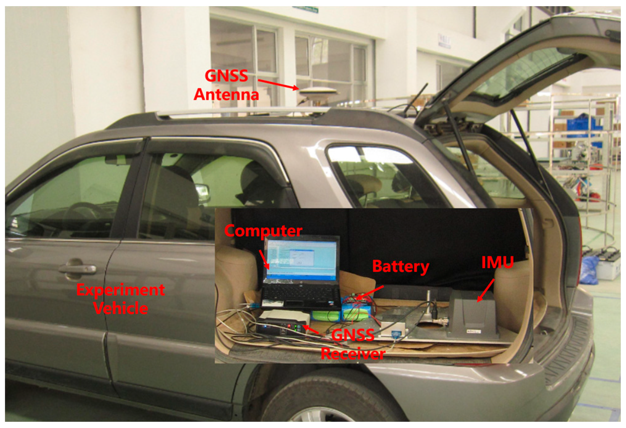
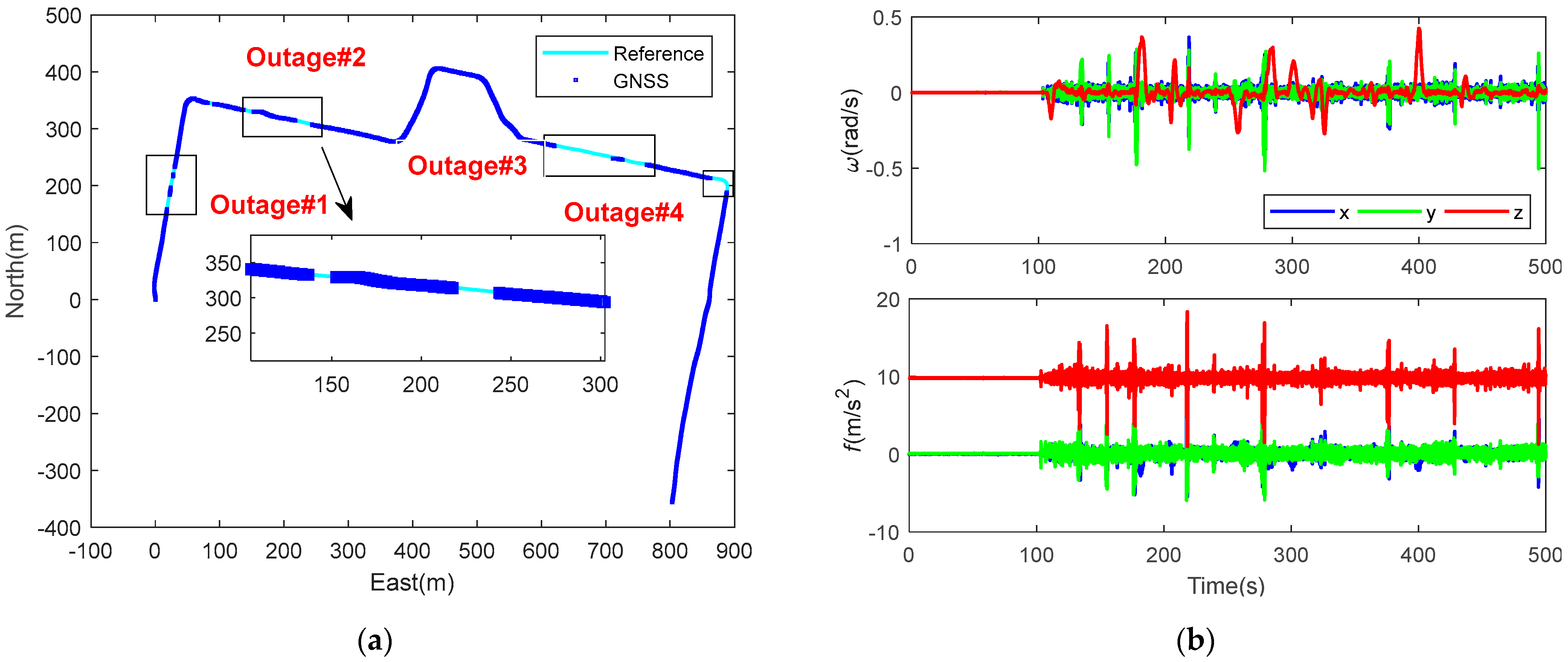
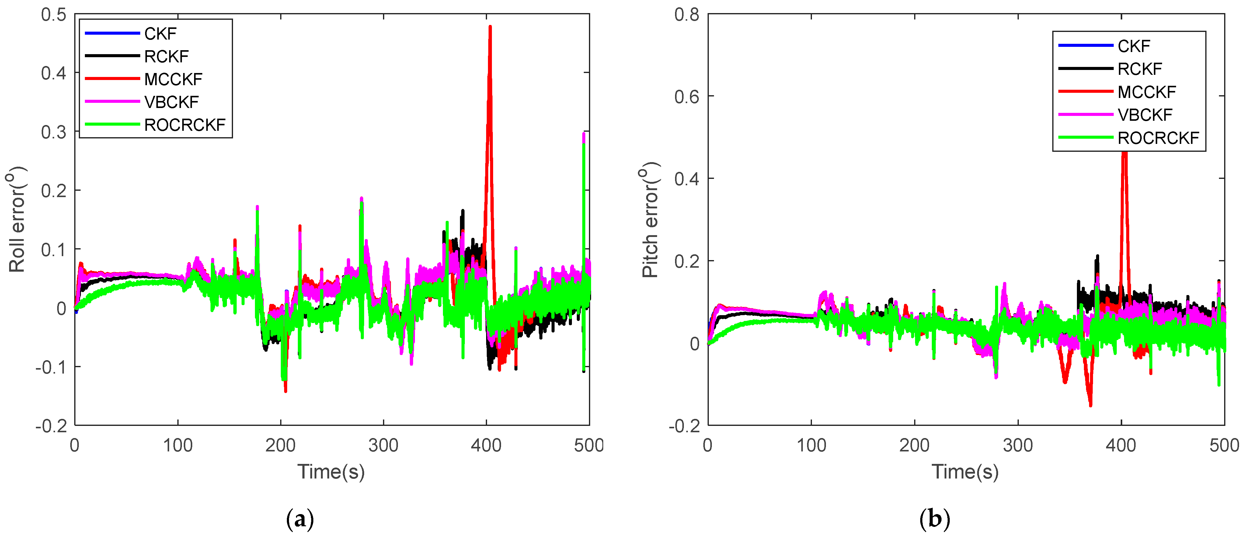
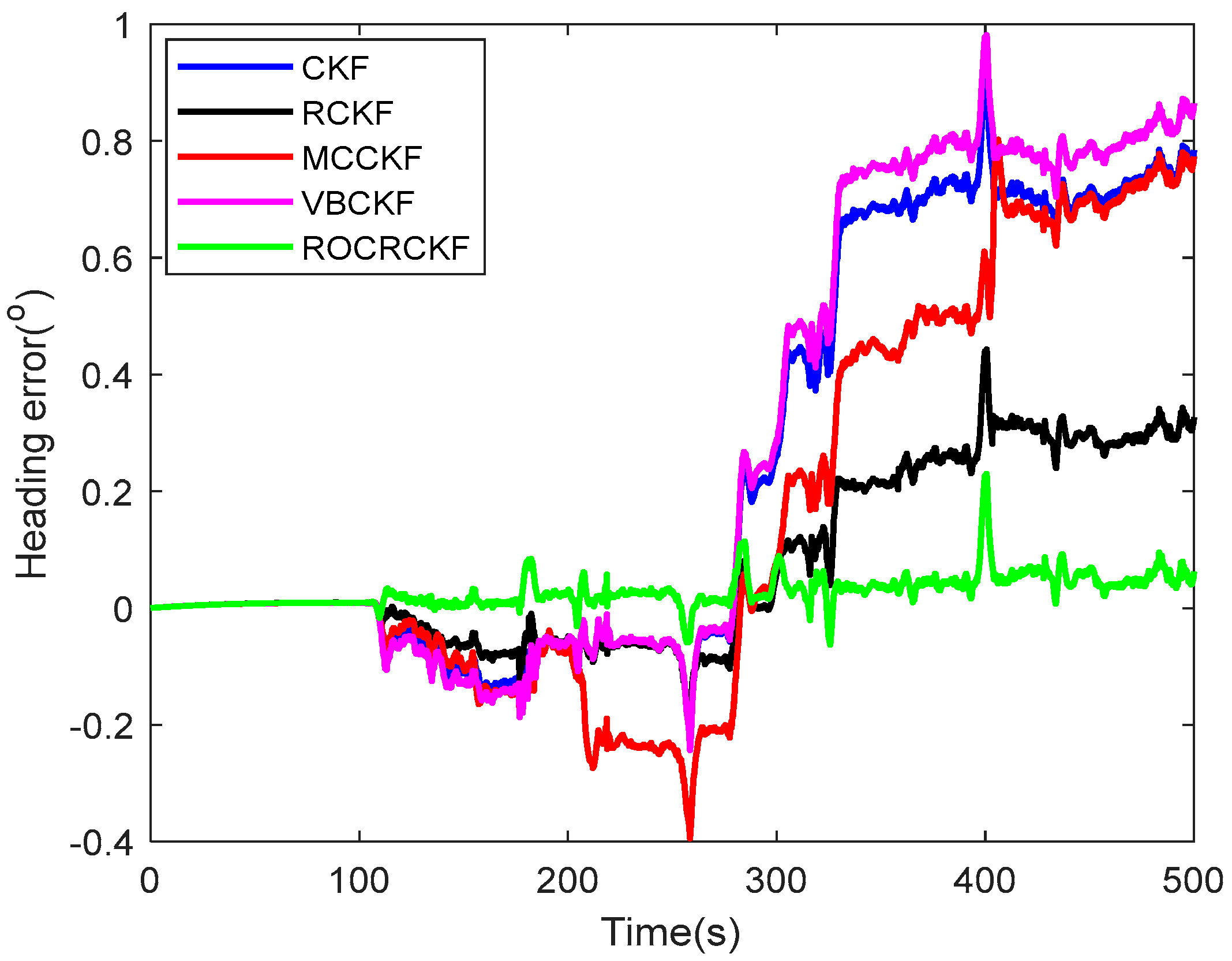
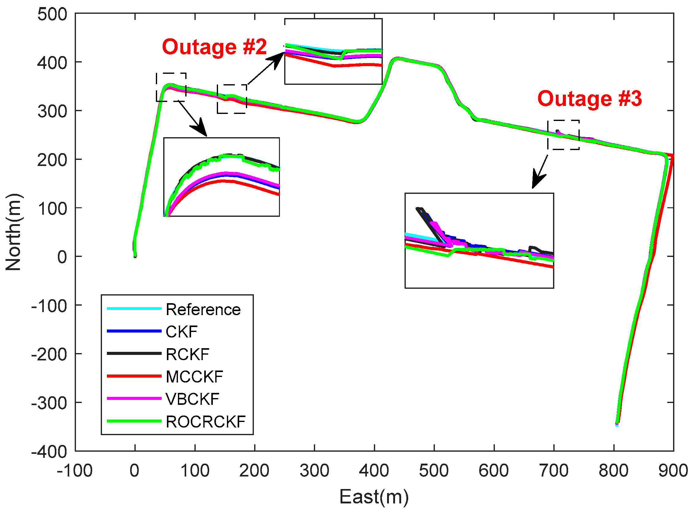
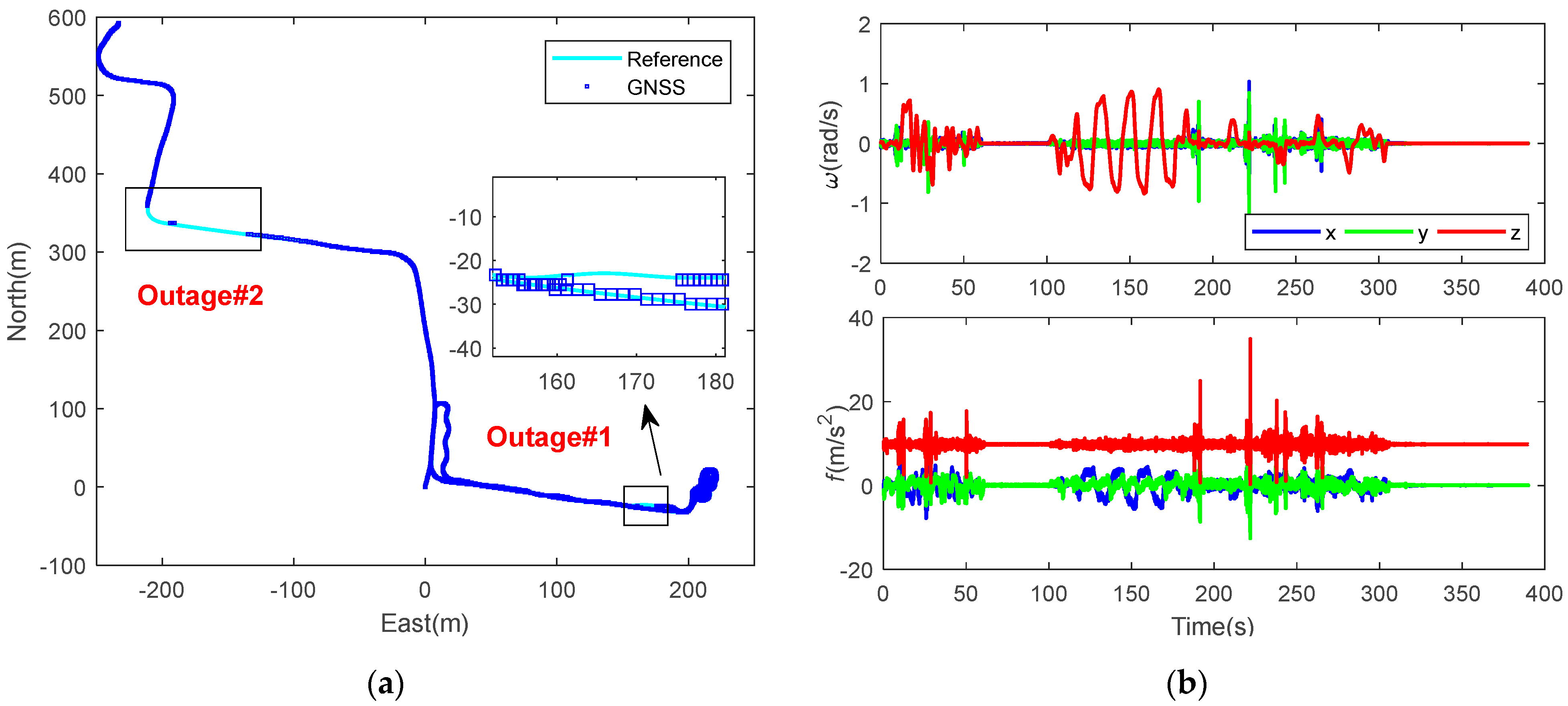
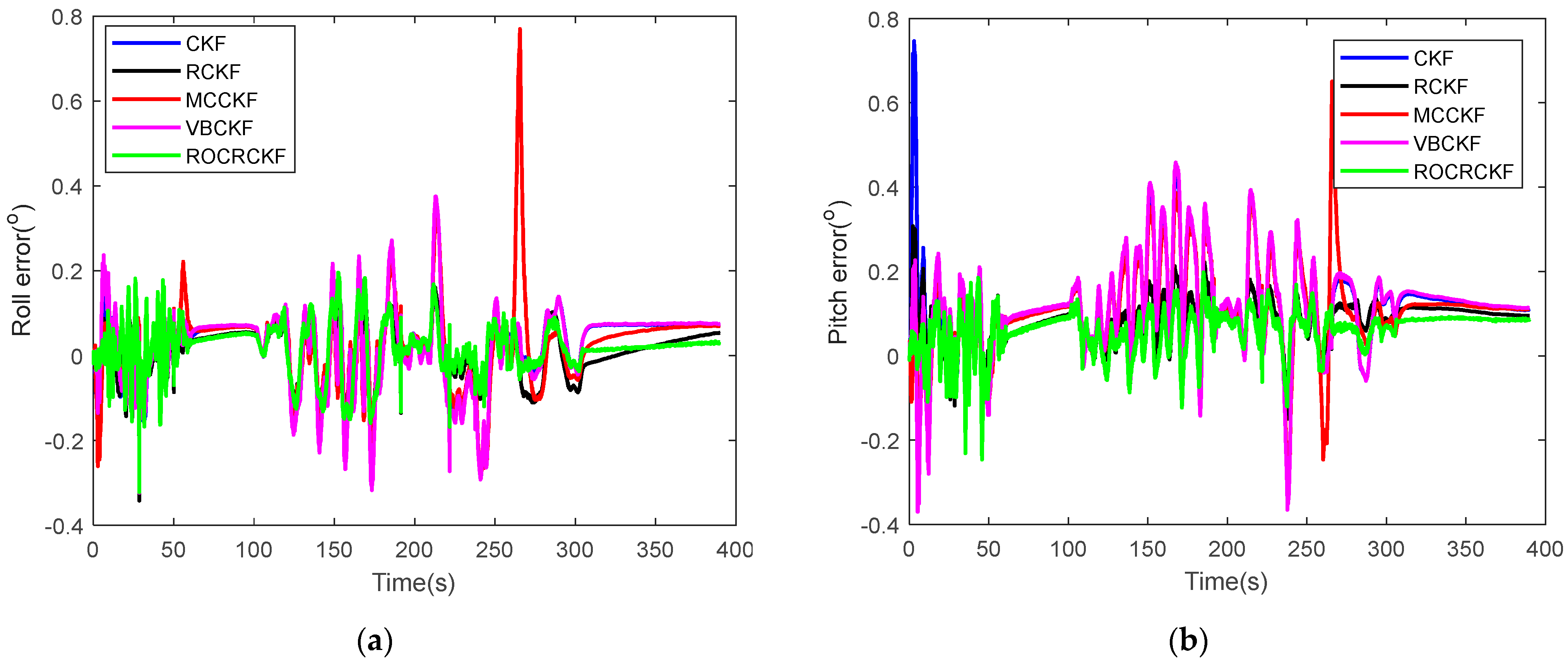
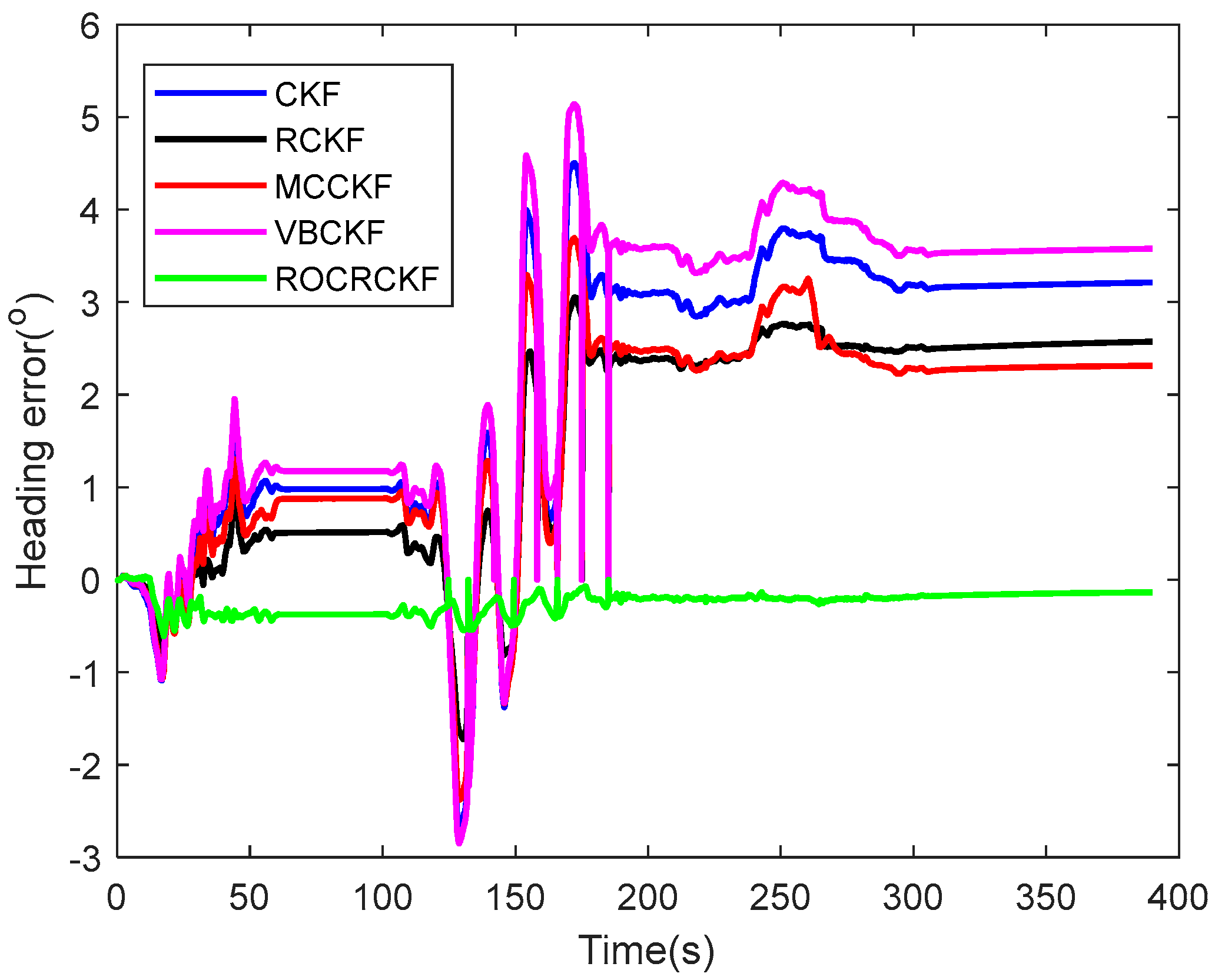
4.2. Experiment and Result Analysis

The experimental vehicle and setups for the field test are shown in Figure 1, where the raw sensor data of the NovAtel SPAN system were first recorded, then post-processed by the Inertial Explorer (IE) software of NovAtel and proposed as nonlinear filters, respectively. In cases where the SPAN system operates in the GNSS/INS tightly coupled mode, it outputs the position and heading continuously within 2 cm and 0.02 degrees, which are taken as the reference trajectories in this work. The IMU of the involved SPAN system includes a triaxial interferometric fiber optic gyroscope and a triaxial MEMS accelerometer; the specific parameters of the IMU are listed in Table 1. The frequencies of the GNSS, IMU, and reference trajectory are 5 Hz, 200 Hz, and 100 Hz.
In this section, two trajectories are employed to verify the observability-constrained resampling-free SUF and outlier-robust measurement update of the ROCRCKF. The VBCKF [19], MCCKF [23], and RCKF [31] are employed as comparisons to verify the superiority of the ROCRCKF in terms of adaptivity and robustness. The forgetting factor is set as ρ = 1 e x p ( 4 ) and the iteration number is J m a x = 20 for the VBCKF and ROCRCKF. The other parameters of the ROCRCKF are e 0 = 0.85 , the dof v k = 5 , t 0 | 0 = p + 1 + τ , T 0 | 0 = τ · R 0 , and τ = 3 . R 0 denotes the initial measurement noise covariance for the VBCKF and ROCRCKF, and is also the constant noise covariance for the CKF, MCCKF, and RCKF. The kernel bandwidth and iteration number of the MCCKF are selected as 400 and 4. The same Λ k is set for the RCKF and ROCRCKF, where for position and velocity, the corresponding η values are set as 1.01 and the other diagonal elements of Λ k are set as 0. The other parameters in the filter settings, except for the above-mentioned parameters, share the same values, and all of the parameters are pre-determined by a series of tuning attempts to make a fair comparison.
The first trajectory is shown in Figure 2, where there are frequent GNSS outages in the test, during which the filters work on prediction mode and thus the SUF based on the approximated moments of the posterior PDF is less efficient. The raw IMU output is shown on the right panel, indicating that the vehicle is still at the initial stage of the test, where ω and f denote the angular rate and specific force. Notably, because of the turning and vibration of the land vehicle there are obvious outliers in the observations of the IMU. Figure 3, Figure 4 and Figure 5 compare the attitude and position error of different nonlinear filters. Notably, the ROCRCKF showcases better performance than the RCKF in terms of attitude, which not only converges faster at the initial stage but also achieves smaller stability errors. It is well recognized that the gyroscope bias in the direction of gravity is unobservable when the land vehicle runs along a straight horizontal line at constant velocity [40]. Consequently, the heading error accumulates with time in cases where the land vehicle runs along a straight line at a constant speed.
The output trajectories of different nonlinear filters for trajectory I are shown in Figure 6. As we can see from the regional enlarged views in Figure 6, both the RCKF and ROCRCKF showcase better position results than the VBCKF and CKF during the turn, which is not only because the accelerometer bias is well compensated but also because the velocity propagation error is reduced by the small heading error. The observability of the heading is low even during steady turns, whereas its accuracy can be improved due to the enhanced observability of tilt angles. Notably, the RCKF performs better than the ROCRCKF in the occurrence of Outage #2, where the outage duration is short enough (less than 10 s) and there are sufficient observations for the RCKF converge to the steady state before another outage. However, in cases where the outage duration is increased, e.g., longer than 30 s, as shown in Outage #3, once the observations are occasionally provided, the RCKF cannot assimilate the innovation efficiently and shows degraded performance compared to the CKF and VBCKF. The sigma points of the CKF, VBCKF, and MCCKF depend on the time update stage of the KF framework, which leads to filtering divergence gradually because of the uncompensated dynamic uncertainty. However, this is not the case for resampling-free SUFs, which modify the sigma points based on (23) by considering the state observability and propagating more information by using the prediction residue of the dynamic model.
More specific estimation results of different filters are listed in Table 2. The root mean square error (RMSE) is formulated as:
RMSE χ = 1 M k = 1 M ( χ ^ k χ k ) 2
where M is the total number of data sets, χ indicates the corresponding navigation state, and χ ^ k and χ k denote the estimated and reference values at time k, respectively. The average RMSE(ARMSE) is taken as the performance metric for the position result, which is defined as:
ARMSE p o s = 1 2 ( RMSE E P 2 + RMSE N P 2 )
where RMSE E P and RMSE N P denote the RMSE of positions in the east and north directions. Notably, in the enlarged image of the left panel of Figure 5, the ROCRCKF converges quickly at the initial stage of the trajectory in cases where the vehicle does not move. By efficiently assimilating the innovation and relieving the covariance inconsistence problem, the ROCRCKF shows better attitude and heading results than its resampling SUF-based counterparts. However, as there is no extra correction information for the states of strong observability during GNSS outages, the ROCRCKF does not improve the position and velocity results compared with the RCKF.
The second trajectory is presented in Figure 7, where the navigation state observability is time-varying and the observability of the attitude is enhanced by frequent maneuver variation. The same parameters as that of trajectory I are employed in the filter configuration and only the observations are different for the comparative analysis of the observability-constrained resampling-free SUF. The results in terms of attitude and position are shown in Figure 8, Figure 9 and Figure 10. Notably, compared with the CKF, the VBCKF achieves slightly better position results but not better attitude results. Both the RCKF and ROCRCKF outperform the VBCKF in terms of attitude and position, and the MCCKF suffers from GNSS outages more obviously than the CKF and VBCKF, which coincides with the results shown in trajectory I. The MCCKF re-scales the uncertainty propagation of measurement updates based on the kernel function, whose performance heavily depends on the selection of kernel parameters, which is less effective in handling non-stationary non-Gaussian noise. Notably, in cases where the car is stopped, the observability constraint causes the direct observable state to approach the actual condition of the vehicle maneuver, which can be seen from the position result in Figure 10. However, the correction information of attitude error and sensor biases comes from prediction covariance, and both the RCKF and the ROCRCKF achieve better attitude results than their resampling-based SUF counterparts.
The output trajectories of different nonlinear filters for trajectory II are shown in Figure 11. As we can see from the regional enlarged views in Figure 11, the ROCRCKF showcases better position results than the RCKF and VBCKF during the turn (Outage #2), which coincides with the result presented in trajectory I. The MCCKF showcases better results than the RCKF, which may be because the MCCKF assimilates the occasionally provided observations efficiently, and the unmodeled dynamic model can be neglected when the vehicle runs in a straight line. The heading accuracy is improved due to the enhanced observability of tilt angles during the frequent turns shown in Figure 11, and thus during Outage #1 all the algorithms achieve acceptable position results. More specific results are listed in Table 3. Notably, the heading and position errors of the CKF are reduced from 2.6° and 7.3 m to 1.96° and 6.38 m by the RCKF, where the position improvement is more significant than that of the VBCKF. The RCKF reduces the ARMSEpos of the VBCKF by 10.5%, where the corresponding value for the first trajectory is 1.2%, which confirms that the resampling-free SUF based on the dynamic prediction residue propagates more information than the SUF based on approximated Gaussian moments. Furthermore, the ROCRCKF outperforms the RCKF and VBCKF in both attitude and position results, where it reduces the position error by 6.7% and 16.5%, respectively. Compared with the results in Table 2, the attitude and heading results of the ROCRCKF shown in Table 3 do not degrade as heavily as those of the RCKF and VBCKF using the same filter configuration, which demonstrates the adaptivity and robustness of the ROCRCKF.

5. Discussion

Notably, the RCKF does not outperform the CKF and VBCKF in terms of roll and pitch in case the maneuver of vehicle is not high, whereas it achieves better position and heading results, especially when there is a GNSS outage. On one hand, the RCKF relieves the covariance inconsistence problem of the CKF by setting the Λ k when constructing the posterior sigma points, which makes the prediction covariance less sensitive to the change in innovation; on the other hand, it cannot assimilate the observation information efficiently once the measurement noise is small enough. The VBCKF improves the position result slightly compared with the CKF, which, however, does not outperform the CKF in terms of attitude and heading. This result coincides with the fact that the correction information of attitude comes from the off-diagonal element of prediction state covariance, which is updated at the prediction stage of nonlinear filters. The estimation results of the MCCKF have a direct relation to the duration of the outage, and in the field test based on trajectory I, it achieves similar heading results as the CKF but much worse position results, which indicates that the MCC-based measurement update cannot address the uncertainty propagation in cases of frequent GNSS outages. Generally, the measurement outliers are sparse in the GNSS/INS, and in cases where the noise is subject to Gaussian distribution, the MCC-based measurement update is sub-optimal and does not perform well. However, in Table 3, unlike the result listed in Table 2, the MCCKF achieves better heading and position results than the CKF and VBCKF, which indicates that the uncertainty or non-Gaussian process noise from the dynamic model has a significant effect on the state estimation of the GNSS/INS.
Notably, in Figure 5 and Figure 10 the position error of the ROCRCKF in the north direction are noisy, and the position error may increase abruptly when the observations reappear after a GNSS outage. The reason behind these phenomena may be that the measurement outlier in different direction behaves differently, whereas the same scalar scale λ k is applied for E ( j ) [ R k ] . The estimation results of the binary indicator E ( j ) [ y k ] and corresponding noise covariance of the position for trajectory II are shown in Figure 12. Notably, the GNSS outages are detected accurately as they coincide with the outages indicated in the left panel of Figure 7. Moreover, the noise covariance diagonal element is increased in the presence of missing observations. Although there is no state update during the GNSS outage, the parameters in Φ k are propagated in the prediction model during these periods, which is also helpful for the sigma point direct modification of the ROCRCKF. As we can see, based on the same filter model, filter configuration, and sensors, the state estimation result of trajectory II is worse than that of trajectory I, which indicates the unmodeled dynamic uncertainty has a significant effect on the state estimation of the GNSS/INS. The comparison analysis between trajectory I and II indicates that the Λ k should be adjusted according to the instantaneous state observability, and thus the observability quantifying analysis based on the real-time degree of observability calculation is under consideration.

6. Conclusions

This article presented an improved observability-constrained resampling-free CKF, the ROCRCKF, for the state estimation of a GNSS/INS with measurement outliers. The binary indicator of outliers, scale parameter of noise covariance, and state are estimated simultaneously based on variational Bayesian inferences. The proposed algorithm is verified by employing a car-mounted GNSS/INS, where two trajectories of different state observability are analyzed and compared. Experiment results demonstrate that, cases where there are frequent GNSS outages, the ROCRCKF outperforms the RCKF and VBCKF in terms of attitude without obvious position degradation. Moreover, when there is high uncertainty in the dynamic model prediction, the ROCRCKF achieves much better results than the RCKF and VBCKF in terms of heading and position results. The vehicle dynamic model-derived measurement should also be taken into consideration for the information fusion of land vehicle navigation, and the dynamic model prediction residue employed in the resampling-free SUF provided a new measure for the vehicle dynamic identification. In future works, multiple indicators of outliers should be employed, as the measurement outliers and noise characteristics may be independent in the observation domain.

Author Contributions

Conceptualization, B.C. and D.W.; methodology, B.C. and X.W.; software, B.C. and Z.S.; validation, B.C. and D.W.; formal analysis, X.W.; investigation, W.C.; resources, B.C. and Y.Z.; data curation, Y.L.; writing—original draft preparation, B.C.; writing—review and editing, W.C. and X.W.; supervision, W.C.; funding acquisition, B.C. and D.W. All authors have read and agreed to the published version of the manuscript.

Funding

This research was jointly funded by the Natural Science Foundation of China, grant number 32271999, the Jiangsu Province and Education Ministry Co-sponsored Synergistic Innovation Center of Modern Agricultural Equipment, grant number XTCX2009, the Primary Research & Development Plan of Jiangsu Province, grant number BE2021313, the Key Laboratory of Spectroscopy Sensing, Ministry of Agriculture and Rural Affairs, grant number 2022ZJUGP002, the University Grants Committee of Hong Kong under the scheme Research Impact Fund on the project R5009-21, and the Research Institute of Land and Space, Hong Kong Polytechnic University. The APC was funded by XTCX2009.

Data Availability Statement

The data presented in this study are available on request from the corresponding author. The data are not publicly available due to the privacy of the subjects involved in the study.

Acknowledgments

We thank the reviewers and editors for their insightful comments that helped to improve the quality of the paper a great deal.

Conflicts of Interest

The authors declare no conflict of interest.

References

  1. Zhang, Q.; Chen, Q.J.; Xu, Z.P.; Zhang, T.S.; Niu, X.J. Evaluating the navigation performance of multi-information integration based on low-end inertial sensors for precision. Precis. Agric. 2021, 22, 627–646. [Google Scholar] [CrossRef]
  2. Falco, G.; Nicola, M.; Pini, M. Positioning based on tightly coupled multiple sensors: A practical implementation and experimental assessment. IEEE Access 2018, 6, 13101–13116. [Google Scholar] [CrossRef]
  3. Kalman, R.E. A new approach to linear filtering and prediction problems. Trans. ASME D J. Basic Eng. 1960, 82, 35–45. [Google Scholar] [CrossRef]
  4. Schmidt, S.F. The Kalman filter: Its recognition and development for aerospace application. J. Guid. Control 1981, 4, 4–7. [Google Scholar] [CrossRef]
  5. Julier, S.J.; Uhlman, J.K.; Durrant-Whyte, H.F. A new method for the nonlinear transformation of means and covariances in filters and estimation. IEEE Trans. Autom. Control 2000, 45, 477–482. [Google Scholar] [CrossRef]
  6. Ito, K.; Xiong, K.Q. Gaussian filters for nonlinear filtering problems. IEEE Trans. Autom. Control 2000, 45, 910–927. [Google Scholar] [CrossRef]
  7. Arasaratnam, I.; Haykin, S. Cubature Kalman filters. IEEE Trans. Autom. Control 2009, 54, 1254–1269. [Google Scholar] [CrossRef]
  8. Crassidis, J.L. Sigma-point Kalman filtering for integrated GPS and inertial navigation. IEEE Trans. Aerosp. Electron. Syst. 2006, 42, 750–756. [Google Scholar] [CrossRef]
  9. Zhao, Y.W. Performance evaluation of cubature Kalman filter in a GPS/IMU tightly-coupled navigation system. Signal Process. 2016, 119, 67–79. [Google Scholar] [CrossRef]
  10. Li, Z.; Li, S.; Liu, B.; Yu, S.S.; Shi, P. A stochastic event-triggered robust cubature Kalman filter filtering approach to power system dynamic state estimation with non-Gaussian measurement noise. IEEE Trans. Control Syst. Technol. 2023, 31, 889–896. [Google Scholar] [CrossRef]
  11. Arulampalam, M.S.; Maskell, S.; Gordon, N.; Clapp, T. A tutorial on particle filters for online nonlinear/non-Gaussian Bayesian tracking. IEEE Trans. Signal Process. 2002, 50, 174–188. [Google Scholar] [CrossRef]
  12. Schön, T.; Gustafsson, F.; Nordlund, P.-J. Marginalized particle filters for mixed linear/nonlinear state-space models. IEEE Trans. Signal Process. 2002, 53, 2279–2289. [Google Scholar] [CrossRef]
  13. Vouch, O.; Minetto, A.; Falco, G.; Dovis, F. On the adaptivity of unscented particle filter for GNSS/INS tightly-integrated navigation unit in urban environment. IEEE Access 2021, 9, 144157–144170. [Google Scholar] [CrossRef]
  14. Gao, G.L.; Gao, B.B.; Gao, S.S.; Hu, G.G.; Zhong, Y.M. A hypothesis test-constrained robust Kalman filter for INS/GNSS integration with abnormal measurement. IEEE Trans. Veh. Technol. 2023, 72, 1662–1673. [Google Scholar] [CrossRef]
  15. Hu, G.G.; Gao, B.B.; Zhong, Y.M.; Gu, C.F. Unscented Kalman filter with process noise covariance estimation for vehicular INS/GPS. Inf. Fusion 2020, 64, 194–204. [Google Scholar] [CrossRef]
  16. Gao, X.L.; Luo, H.Y.; Ning, B.K.; Zhao, F.; Bao, L.F.; Gong, Y.L.; Xiao, Y.M.; Jiang, J.G. RL-AKF adaptive Kalman filter navigation algorithm based on reinforcement learning for ground vehicles. Remote Sens. 2020, 12, 1704. [Google Scholar] [CrossRef]
  17. Xue, C.; Huang, Y.L.; Zhu, F.C.; Zhang, Y.G.; Chambers, J.A. An outlier-robust Kalman filter with adaptive selection of elliptically contoured distributions. IEEE Trans. Signal Process. 2022, 70, 994–1009. [Google Scholar] [CrossRef]
  18. Sun, J.; Ye, Q.Q.; Lei, Y. In-motion alignment method of SINS based on improved Kalman filter under geographic latitude uncertainty. Remote Sens. 2022, 14, 2581. [Google Scholar] [CrossRef]
  19. Särkkä, S.; Nummenmaa, A. Recursive adaptive Kalman filtering by variational Bayesian approximations. IEEE Trans. Autom. Control 2009, 54, 596–600. [Google Scholar] [CrossRef]
  20. Cui, B.B.; Chen, X.Y.; Xu, Y.; Huang, H.Q.; Liu, X. Performance analysis of improved iterated cubature Kalman filter and its application to GNSS/INS. ISA Trans. 2017, 66, 460–468. [Google Scholar] [CrossRef]
  21. Huang, Y.L.; Zhang, Y.G.; Wu, Z.M.; Li, N.; Chambers, J. A novel adaptive Kalman filter with inaccurate process and measurement noise covariance matrices. IEEE Trans. Autom. Control 2018, 63, 594–601. [Google Scholar] [CrossRef]
  22. Chang, L.B.; Li, K.L.; Hu, B.Q. Huber’s M-estimation-based process uncertainty robust filter for integrated INS/GPS. IEEE Sens. J. 2015, 15, 3367–3374. [Google Scholar] [CrossRef]
  23. Chen, B.D.; Liu, X.; Zhao, H.Q.; Principe, J.C. Maximum correntropy Kalman filter. Automatica 2017, 76, 70–77. [Google Scholar] [CrossRef]
  24. Liu, D.; Chen, X.Y.; Xu, Y.; Liu, X.; Shi, C.F. Maximum correntropy generalized high-degree cubature Kalman filter with application to the attitude determination system of missile. Aerosp. Sci. Technol. 2019, 95, 105441. [Google Scholar] [CrossRef]
  25. Shmaliy, Y.S. Linear optimal FIR estimation of discrete time-invariant state-space models. IEEE Trans. Signal Process. 2010, 58, 3086–3096. [Google Scholar] [CrossRef]
  26. Shmaliy, Y.S. Predictive tracking under persistent disturbances and data error using H2 FIR approach. IEEE Trans. Ind. Electron. 2022, 69, 6121–6129. [Google Scholar] [CrossRef]
  27. Nurminen, H.; Ardeshiri, T.; Piché, R.; Gustafsson, F. Skew-t filter and smoother with improved covariance matrix approximation. IEEE Trans. Signal Process. 2018, 66, 5618–5633. [Google Scholar] [CrossRef]
  28. Zhu, H.; Zhang, G.R.; Li, Y.F.; Leung, H. A novel robust Kalman filter with unknown non-stationary heavy-tailed noise. Automatica 2021, 127, 109511. [Google Scholar] [CrossRef]
  29. Huang, Y.L.; Zhang, Y.G.; Zhao, Y.; Chambers, J.A. A novel robust Gaussian-Student’s t mixture distribution based Kalman filter. IEEE Trans. Signal Process. 2019, 67, 3606–3620. [Google Scholar] [CrossRef]
  30. Fu, H.P.; Huang, W.; Li, Z.W.; Cheng, Y.M.; Zhang, T.Y. Robust cubature Kalman filter with Gaussian-multivariate Laplacian mixture distribution and partial variational Bayesian method. IEEE Trans. Signal Process. 2023, 71, 847–858. [Google Scholar] [CrossRef]
  31. Cui, B.B.; Chen, X.Y.; Tang, X.H. Improved cubature Kalman filter for GNSS/INS based on transformation of posterior sigma-points error. IEEE Trans. Signal Process. 2017, 65, 2975–2987. [Google Scholar] [CrossRef]
  32. Wang, M.S.; Wu, W.Q.; Zhou, P.Y.; He, X.F. State transformation extended Kalman filter for GPS/SINS tightly coupled integration. GPS Solut. 2018, 22, 112. [Google Scholar] [CrossRef]
  33. Yang, Y.L.; Huang, G.Q. Observalility analysis of aided INS with heterogeneous features of points, lines, and planes. IEEE Trans. Robot. 2019, 35, 1399–1418. [Google Scholar] [CrossRef]
  34. Cui, B.B.; Wei, X.H.; Chen, X.Y.; Li, J.Y.; Wang, A.C. Robust cubature Kalman filter based on variational Bayesian and transformed posterior sigma points error. ISA Trans. 2019, 86, 18–28. [Google Scholar] [CrossRef]
  35. Wang, G.W.; Cui, B.B.; Tang, C.Y. Robust cubature Kalman filter based on maximum correntropy and resampling-free sigma-point update framework. Digital Signal Process. 2022, 126, 103495. [Google Scholar] [CrossRef]
  36. Wang, H.W.; Li, H.B.; Fang, J.; Wang, H.P. Robust Gaussian Kalman filter with outlier detection. IEEE Signal Process. 2018, 25, 1236–1240. [Google Scholar] [CrossRef]
  37. Li, H.Q.; Medina, D.; Vilà-Valls, J.; Closas, P. Robust variational-based Kalman filter for outlier rejection with correlated measurement. IEEE Trans. Signal Process. 2021, 69, 357–369. [Google Scholar] [CrossRef]
  38. Straka, O.; Dunik, J. Resampling-free stochastic integration filter. In Proceedings of the IEEE 23rd International Conference on Information Fusion (FUSION), Sun City, South Africa, 6–9 July 2020. [Google Scholar]
  39. Groves, P.D. Principles of GNSS, Intertial, and Multisensory Integrated Navigation Systems, 2nd ed.; Artech House: Boston, MA, USA, 2008; pp. 382–393. [Google Scholar]
  40. Hong, S.; Lee, M.H.; Chun, H.H.; Kwon, S.H.; Speyer, J.L. Observability of error states in GPS/INS integration. IEEE Trans. Veh. Technol. 2005, 54, 731–743. [Google Scholar] [CrossRef]
Figure 1. Experimental setup for field test data recording.
Remotesensing 15 04591 g001
Figure 2. Raw observations of the GNSS and IMU data of trajectory I. (a) Trajectory of the field test with frequent GNSS outages, some of which are flagged in the rectangle and shown in an enlarged view; (b) Raw IMU output data indicating a stop at the initial stage of the trajectory.
Remotesensing 15 04591 g002
Figure 3. Result of attitude estimation for trajectory I. (a) The roll error of different nonlinear filters; (b) The pitch error of different nonlinear filters.
Remotesensing 15 04591 g003
Figure 4. Result of heading estimation for trajectory I.
Remotesensing 15 04591 g004
Figure 5. Result of position estimation for trajectory I. (a) The east position error of different nonlinear filters; (b) The north position error of different nonlinear filters.
Remotesensing 15 04591 g005
Figure 6. Output trajectories of different nonlinear filters for trajectory I.
Remotesensing 15 04591 g006
Figure 7. Raw observations of GNSS and IMU data of trajectory II. (a) Trajectory of field test with GNSS outages, some of which are flagged in the rectangle and shown in an enlarged view; (b) Raw IMU output data indicating there are two still periods in the trajectory.
Remotesensing 15 04591 g007
Figure 8. Results of attitude estimation for trajectory II. (a) The roll error of different nonlinear filters; (b) The pitch error of different nonlinear filters.
Remotesensing 15 04591 g008
Figure 9. Results of heading estimation for trajectory II.
Remotesensing 15 04591 g009
Figure 10. Results of position estimation for trajectory II. (a) The east position error of different nonlinear filters; (b) The north position error of different nonlinear filters.
Remotesensing 15 04591 g010
Figure 11. Output trajectories of different nonlinear filters for trajectory II.
Remotesensing 15 04591 g011
Figure 12. Result of binary indicator and measurement noise covariance estimation.
Remotesensing 15 04591 g012
Table 1. Parameter information of the IMU.
SensorCharacteristicValue
GyroscopeRate bias1 deg/h
Rate scale factor100 ppm
Angular random walk0.07 deg/ h
AccelerometerBias0.3 mg
Scale factor300 ppm
Table 2. The RMSEs of different nonlinear filters for trajectory I.
MethodRoll (°)Pitch (°)Heading (°)ARMSEpos (m)
CKF0.0450.0590.442.61
RCKF0.0450.0650.172.50
MCCKF0.0590.0800.385.48
VBCKF0.0460.0590.482.53
ROCRCKF0.0300.0410.042.55
Table 3. The RMSEs of different nonlinear filters for trajectory II.
MethodRoll (°)Pitch (°)Heading (°)ARMSEpos (m)
CKF0.0910.162.607.30
RCKF0.0570.101.966.38
MCCKF0.1050.152.006.18
VBCKF0.0970.162.947.13
ROCRCKF0.0580.080.275.95
Disclaimer/Publisher’s Note: The statements, opinions and data contained in all publications are solely those of the individual author(s) and contributor(s) and not of MDPI and/or the editor(s). MDPI and/or the editor(s) disclaim responsibility for any injury to people or property resulting from any ideas, methods, instructions or products referred to in the content.

