A Novel Discriminative Enhancement Method for Few-Shot Remote Sensing Image Scene Classification

Abstract

Remote sensing image scene classification (RSISC) has garnered significant attention in recent years. Numerous methods have been put forward in an attempt to tackle this issue, particularly leveraging deep learning methods that have shown promising performance in classifying remote sensing image (RSI). However, it is widely recognized that deep learning methods typically require a substantial amount of labeled data to effectively converge. Acquiring a sufficient quantity of labeled data often necessitates significant human and material resources. Hence, few-shot RSISC has become highly meaningful. Fortunately, the recently proposed deep nearest neighbor neural network based on the attention mechanism (DN4AM) model incorporates episodic training and class-related attention mechanisms, effectively reducing the impact of background noise regions on classification results. Nevertheless, the DN4AM model does not address the problem of significant intra-class variability and substantial inter-class similarities observed in RSI scenes. Therefore, the discriminative enhanced attention-based deep nearest neighbor neural network (DEADN4) is proposed to address the few-shot RSISC task. Our method makes three contributions. Firstly, we introduce center loss to enhance the intra-class feature compactness. Secondly, we utilize the deep local-global descriptor (DLGD) to increase inter-class feature differentiation. Lastly, we modify the Softmax loss by incorporating cosine margin to amplify the inter-class feature dissimilarity. Experiments are conducted on three diverse RSI datasets to gauge the efficacy of our approach. Through comparative analysis with various cutting-edge methods including MatchingNet, RelationNet, MAML, Meta-SGD, DN4, and DN4AM, our approach showcases promising outcomes in the few-shot RSISC task.

1. Introduction

Remote sensing image scene classification (RSISC) is a significant undertaking that has attracted considerable interest across diverse domains and use cases [1,2,3]. The continuous evolution of imaging technology has resulted in notable advancements, contributing to the progressive enhancement of resolution in remote sensing images (RSI) [4,5,6]. This encompasses a wide array of intricate land cover characteristics, including terrain, mountains, and bodies of water. The processing of RSI varies depending on the specific characteristics exhibited by the scenes they depict [1]. Assigning semantic labels to RSI holds immense importance as this facilitates the unified management and analysis of remote sensing data. Semantic labels aid in organizing and analyzing these data in a consistent manner. Thus, the primary objective of scene classification is to categorize RSI based on similar scene characteristics using extracted features [7,8,9]. Presently, the usage of scene classification technology extends across a wide range of domains, including but not limited to natural disaster evaluation, vegetation mapping, geological surveying, urban planning, environmental monitoring, object detection, and various other disciplines [10,11,12,13,14,15,16,17].

In recent years, deep learning techniques have gained substantial traction as highly prospective methodologies for RSISC [18], showcasing notable achievements with models like VGG16 [19], GoogLeNet [20], AlexNet [21], and ResNet [22]. Deep learning has revolutionized RSISC by eliminating the need for manual feature retrieval [23,24,25,26]. This approach holds immense significance in remote sensing applications. Recently, Zhai et al. [27] introduced a highly efficient model that addresses the issue of lifelong learning, which incorporates prior knowledge to enable rapid generalization to new datasets. In line with this objective, Zhang et al. [28] incorporated the remote sensing transformer (TRS) into the realm of RSISC, with the primary goal of capturing long-range dependencies and acquiring comprehensive global features from the images. To further enhance the extraction of semantic features from different classes, Tang et al. [29] conducted spatial rotation on RSI based on previous studies. This creative approach helps capture additional valuable information and reduces the potential for misclassification by improving feature discriminability. Harnessing these breakthroughs resulted in substantial improvements in the accuracy and resilience of RSISC, leading to enhanced performance in various applications.

From another perspective, the effectiveness of deep learning approaches is often greatly influenced by the quality and quantity of the available training set. This implies that a substantial amount of human and material resources must be invested in acquiring labeled image data. Additionally, well trained deep learning models are only effective for the scenes included in the training dataset and cannot accurately classify scenes not present in the training set. To incorporate new scenes, it is necessary to include them in the training set and retrain the model.

Therefore, for the problem of scene classification in RSI, few-shot learning becomes highly meaningful. The core issue of few-shot learning revolves around exploring methods to rapidly acquire knowledge from a limited set of annotated samples, with the aim of enabling the model to exhibit rapid learning capabilities [30,31,32]. Given the possibility of utilizing prior knowledge to address this core issue, few-shot learning methods can be classified from three standpoints: (i) data, where prior knowledge enriches the supervised learning process; (ii) model, where prior knowledge diminishes the complexity of the hypothesis space; and (iii) algorithm, where prior knowledge modifies the search for the optimal hypothesis within the provided hypothesis space [30,31,32]. For example, Cheng et al. introduced a Siamese-prototype network (SPNet) with prototype self-calibration (SC) and intercalibration (IC) to tackle the few-shot problem [33]. SC utilizes supervision information from support labels to calibrate prototypes generated from support features, while IC leverages the confidence scores of query samples as additional prototypes to predict support samples, further improving prototype calibration. Chen et al. proposed a novel method named multiorder graph convolutional network (MGCN) [34], which tackles the few-shot scene classification challenge by employing two approaches: mitigating interdomain differences through a domain adaptation technique that adjusts feature dispersion based on their weights, and decreasing the dispersion degree of node features. Therefore, in the few-shot task, the deep features learned by the model should not only have good separability, but also have strong discriminability, so that new classes can be recognized with a limited set of annotated samples. Vin et al. [35] introduced an episodic training approach as a solution to tackle the challenges associated with few-shot learning. In the training stage, a support set is created by randomly selecting K images for each of the C classes that are sampled from the dataset, resulting in a total of $C\times K$ images. Subsequently, N images are chosen from the remaining dataset for each class among the selected C classes, forming a query set. An episode is formed by combining one support set with one query set. Multiple iterations of training using different episodes are performed until convergence, enabling the network to provide the class labels of query set images based on their resemblance to the support set. The predominant approach in metric learning-based few-shot methods entails the direct computation of the distance between support samples and query samples, enabling the subsequent learning of a classifier based on this measured distance. They do not fully exploit the network’s robustness in extracting features, resulting in the reduced discriminability of the model’s output features and consequently hindering the overall performance of few-shot models.

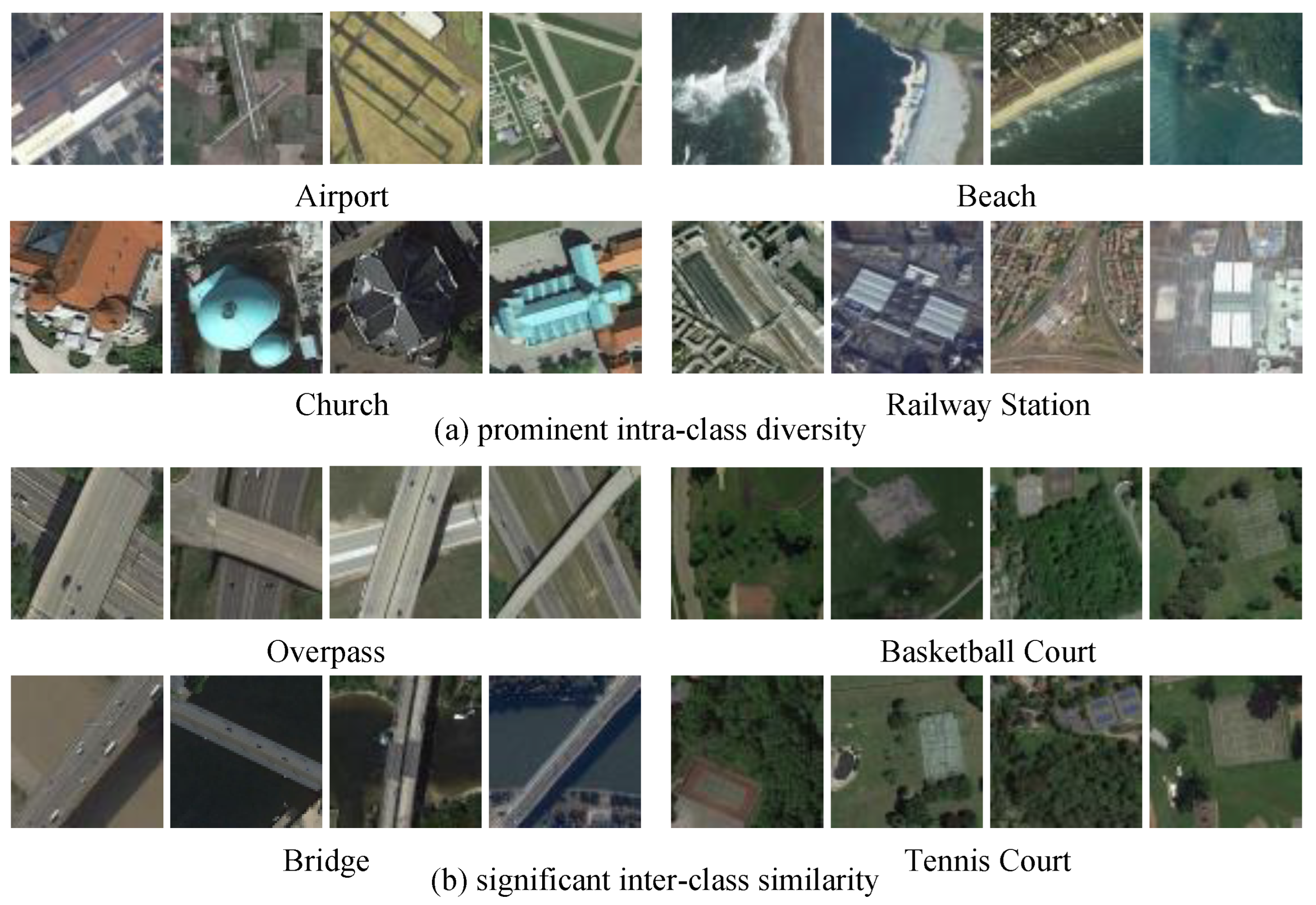
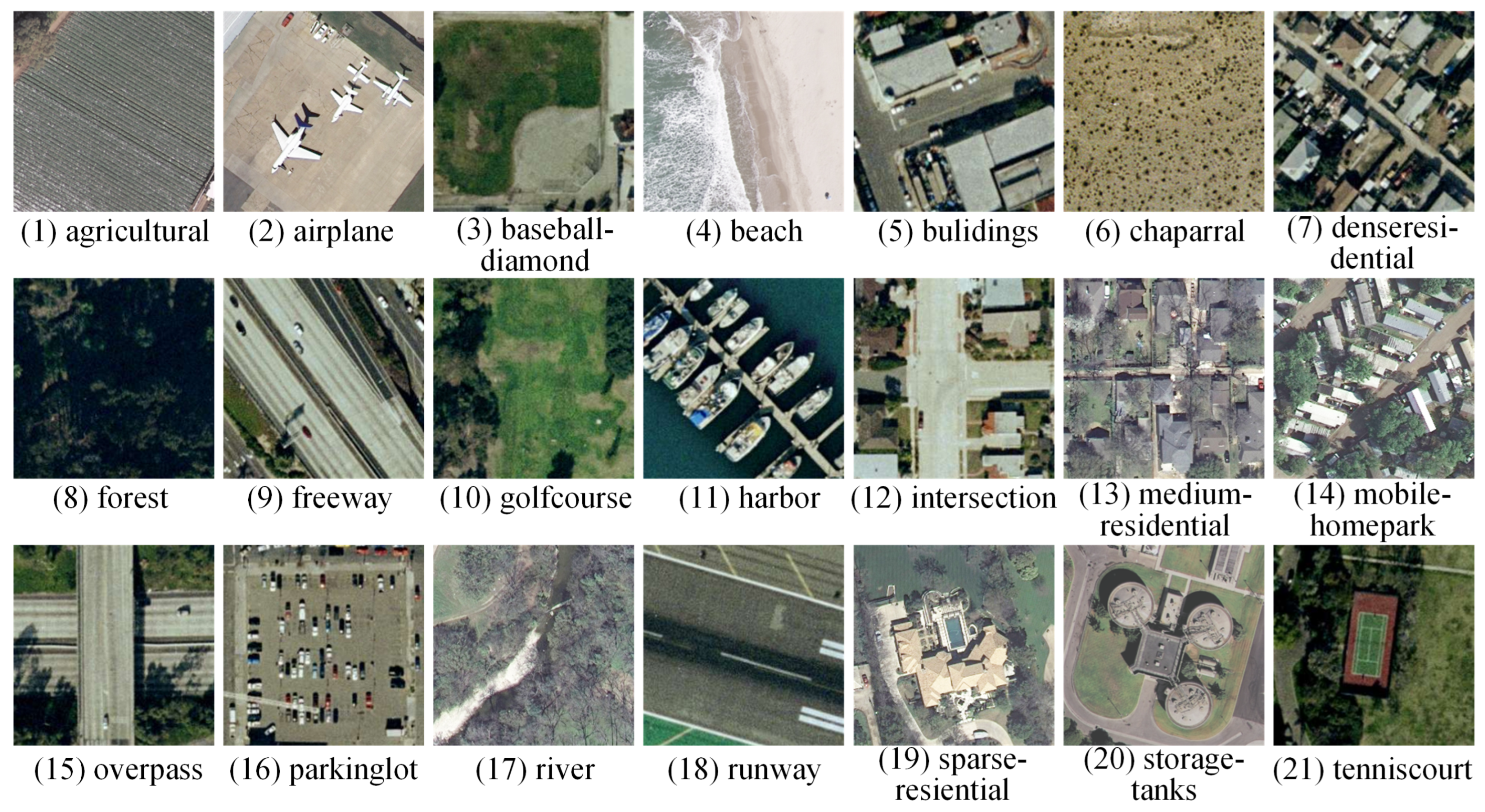
Moreover, RSI frequently presents significant intra-class variations and noticeable inter-class similarities, posing challenges for precise scene image classification. The substantial intra-class variance pertains to the assortment of visual attributes exhibited by objects belonging to the same semantic class. Certain ground-level entities demonstrate variations in terms of style, shape, and spatial distribution. For example, as shown in Figure 1a, churches exhibit diverse architectural styles, while airports and railway stations display notable differences in their distinct shapes. Furthermore, when an airplane or space platform captures a RSI, due to different imaging conditions, the color and radiation intensity in the identical category may be significantly different due to weather, cloud, fog and other factors. For example, beach scenes exhibit significant differences under different imaging conditions. The notable similarities across distinct classes in RSI is primarily due to the presence of similar objects or semantic overlap among different scene classes. For example, in Figure 1b, both bridge and overpass scenes contain the same objects, and basketball court and tennis court exhibit a high degree of semantic information overlap. In addition, the vague definition of scene classes can also lead to reduced inter-class differences, resulting in visually similar appearances for some complex scenes. Therefore, distinguishing between these scene classes can be extremely challenging, which is attributable to the extensive intra-class variations and pronounced inter-class resemblance. For example, images that do not belong to the same class are classified into one class, and different classes may be assigned to images that actually belong to the same class due to the diversity of samples. For this reason, the acquisition of a classifier capable of extracting discriminative features from RSI significantly contributes to enhancing the performance of RSISC.

To solve the few-shot RSISC, Chen et al. [36] proposed the deep nearest neighbor neural network based on attention mechanism (DN4AM). DN4AM employs an episodic training technique for network training and performs evaluations on novel classes to enhance few-shot learning. In addition, DN4AM integrates a channel attention mechanism to craft attention maps that are tailored to scene classes, harnessing global information to mitigate the influence of unimportant regions. Furthermore, DN4AM employs the scene class-related attention maps to measure the resemblance of descriptors between query images and support images. By employing this strategy, DN4AM is able to compute a metric score for each image-to-class comparison, effectively mitigating the impact of irrelevant scene-semantic objects and elevating the classification accuracy. However, DN4AM does not address the challenge of significant intra-class variations and substantial inter-class similarities in RSI scenes.

In this paper, we propose the discriminative enhanced attention-based deep nearest neighbor neural network (DEADN4) based on the DN4AM model. While retaining the advantages of DN4AM, DEADN4 model has three additional advantages. Firstly, incorporating both local and global information, the DEADN4 model employs the deep local-global descriptor (DLGD) for classification, enhancing the differentiation between different classes’ descriptors. Secondly, to enhance the intra-class compactness, DEADN4 introduces the center loss to optimize global information. By using the center loss, it effectively increases the intra-class compactness by pulling features of the same class towards their centers, mitigating significant intra-class diversity. Finally, DEADN4 improves the Softmax loss function in the classification module by incorporating the cosine margin, encouraging larger inter-class distances between learned features. These advantages contribute to improving the few-shot RSISC results. In Section 2, we delve into the existing research in the domain. In Section 3, we unveil our proposed method. The outcomes of our experiments and corresponding discussion are elucidated in Section 4. Lastly, in Section 5, we draw definitive conclusions based on our findings.

2. Related Work

Deep convolutional neural network (CNN) is capable of extracting abundant semantic features and distinguishing diverse classes of deep features in the final fully connected layer of the network, enabling the accurate prediction of test samples. Nevertheless, research has found that traditional Softmax loss can disperse features belonging to different classes as much as possible, but it overlooks the intra-class compactness of features, leading to a deficiency in the discriminability of the learned features. Therefore, many researchers started studying how more discriminative features could be extracted to further enhance the performance of CNN. Intuitively, if the close clustering within classes and the distinct differentiation across classes are maximized simultaneously, the learned features will have excellent separability and discriminability. Although learning good features is not easy for many tasks due to significant inter-class differences, considering the powerful representational capacity of CNN, it is possible to learn features that exhibit both good separability and strong discriminability. At present, the work related to the discriminative enhancement of CNN can be roughly divided into two classes: class-center method and improved loss function. Since our method is based on DN4AM, this section will include a concise overview of the DN4AM model.

2.1. Class-Center Method

The method of using the class-center usually defines a center for each class, and then increases the distinguishability of the model’s extracted features by increasing the intra-class compactness [37,38,39]. The class-center is defined by researchers, and a commonly used definition for the class-center is the average of the characteristics found in training samples belonging to the identical category. Wen et al. [37] believe that CNN can complete classification tasks by using Softmax loss training until the network converges. However, an observation can be made that the acquired features through the network still exhibit significant intra-class variance, indicating that the network’s acquired deep features are separable through solely using Softmax loss but lack sufficient discriminability. Thus, Wen et al. proposed the center loss to augment the distinctiveness of the acquired features within the neural network, which can be formulated as:

$$\begin{array}{cc}\hfill & L_C=\frac{1}{2}\sum _{i=1}^N{∥X_i-c_{y_i}∥}_2^2\hfill \end{array}$$

(1)

where $c_{y_i}\in {\mathbb{R}}^d$ represents the $y_{i}th$ class-center of the deep feature, m denotes the population size of the current training dataset. The combination of Softmax loss and center loss in training the CNN achieves exceptional accuracy on various significant face recognition datasets. The experiments demonstrate that, through the aforementioned joint supervision, a more robust neural network can be trained, obtaining deep features that aim to achieve both the dispersion between different classes and the compactness within same class. This significantly enhances the distinguishability of the extracted features through the deep learning model.

2.2. Improved Loss Function

The loss function is a pivotal area of study in machine learning, greatly influencing the development and enhancement of various machine learning techniques. For classification and recognition tasks, the deep CNN is employed to extract critical information from face images, ensuring that samples within the same class exhibit similarity whereas samples belonging to different classes display pronounced dissimilarity. Softmax loss is commonly used to solve multi-class classification problems, which are widely adopted in practical scenarios like image recognition, face recognition, and semantic segmentation. Although the Softmax loss function is concise and has probabilistic semantics, making it one of the frequently employed elements in CNN models, some scholars argue that it does not overtly advocate for compactness within the same class and distinctiveness between different classes [40,41]. In order to tackle this problem, based on their work [40,41], the loss function of Softmax can be modified as follows:

$$\begin{array}{cc}\hfill & L_s=\frac{1}{N}\sum _i^N-log\frac{e^{s\left(cos\left({\theta }_{y_i,i}\right)-M_m\right)}}{e^{s\left(cos\left({\theta }_{y_i,i}\right)-M_m\right)}+{\sum }_{j\ne y_i}{e}^{scos\left({\theta }_{j,i}\right)}}\hfill \end{array}$$

(2)

where N is the quantity belonging to the training samples, $y_i$ is the class information of the ith sample, ${\theta }_{j,i}$ denotes the deviation angle between the weight vector of the jth class and the ith sample, $M_m\ge 0$ is a constant employed to regulate the cosine margin, s is a fixed value. In this way, the Softmax loss is formulated in terms of cosine, and the cosine margin is utilized to maximize the distance between features in the cosine decision space. As a result, the objective of reducing variability within classes while increasing dissimilarity between classes has been successfully accomplished.

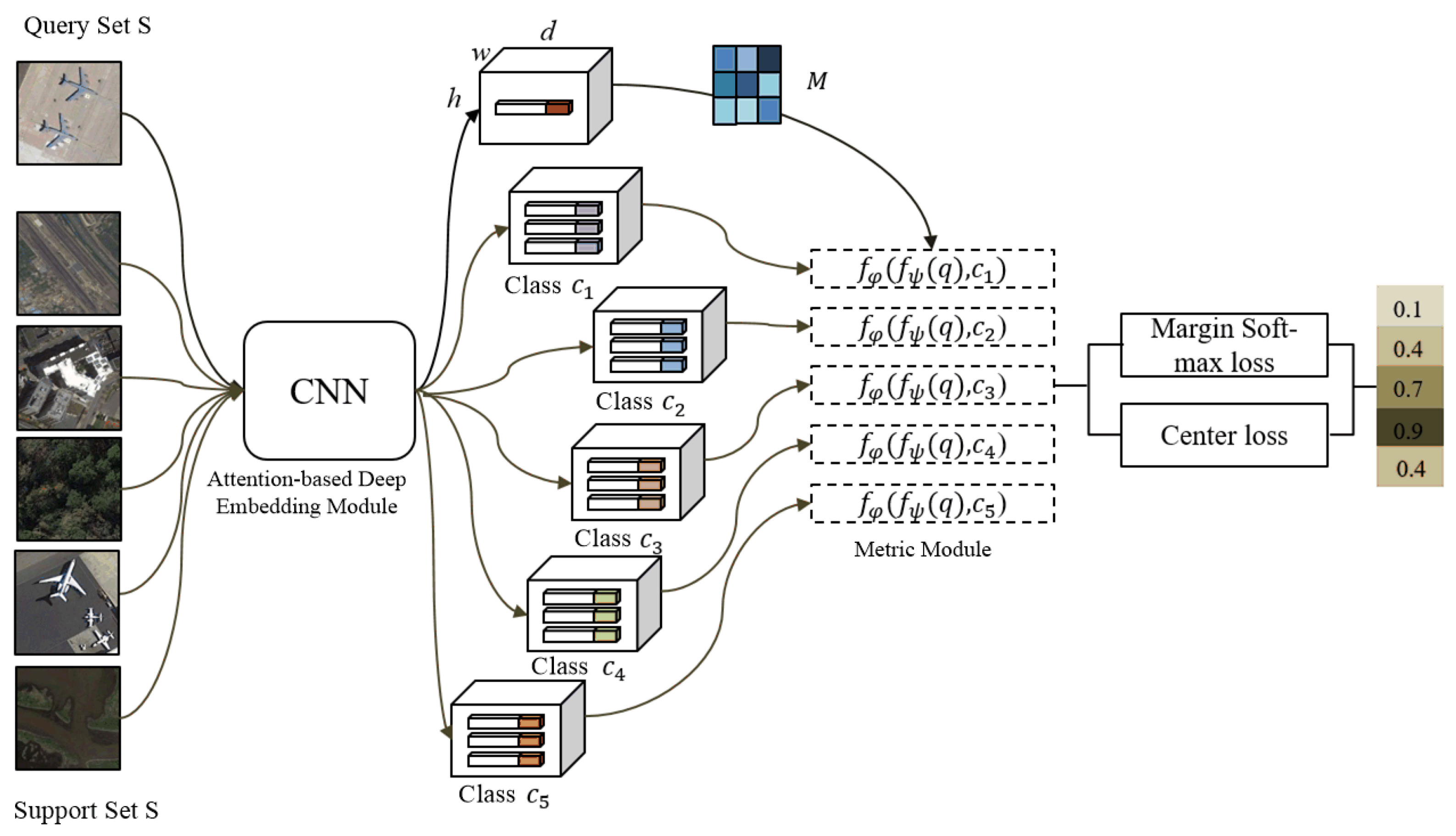
2.3. DN4AM

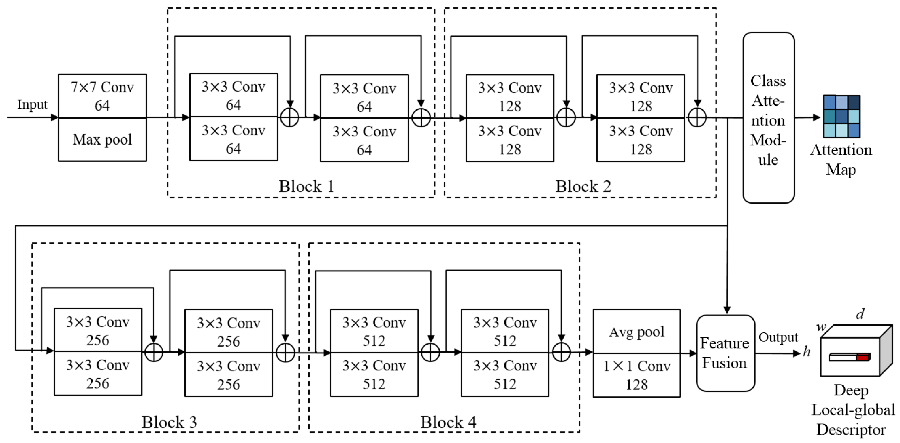
DN4AM is a model designed to address the problem of few-shot RSISCs. It consists of two main parts: attention-based deep embedding module $f_{\psi }(·)$ and the metric module $f_{\phi }(·)$.

The $f_{\psi }(·)$ module is responsible for capturing the deep local descriptor (DLD) within images and generating attention maps that are closely associated with scene classes. For each input image X, $f_{\psi }\left(X\right)$ represents a feature map of size $h\times w\times d_1$, which can be seen as containing $h\times w$ DLD of dimension $d_1$. The DLD captures the features in different regions of the image.

Additionally, the $f_{\psi }(·)$ module incorporates a class-relevant attention learning module. This module partitions the DLD into relevant and irrelevant parts to the scene classification. The primary purpose of this is to minimize the impact of ambient noise and prioritize the characteristics associated with the scene class.

Finally, in the $f_{\phi }(·)$ module, the class of a query image is determined by comparing the similarity between the DLDs of the query and support images.

In summary, DN4AM utilizes the $f_{\psi }(·)$ module to learn the features about scene classes in images. The $f_{\phi }(·)$ module then compares the similarities between query and support images’ DLDs to perform few-shot RSISC. This approach provides more accurate classification results while reducing interference from background noise.

3. Methods

3.1. Architecture

DN4AM improves the network by addressing the issue of interference from irrelevant background noise in few-shot scene classification, but it overlooks intra-class compactness. Our method, which builds upon the foundation of DN4AM, is proposed to tackle the aforementioned problem. The diagram of our method is illustrated in Figure 2. To acquire more stronger features, our method integrates local and global information and performs classification using DLGD. Additionally, the center loss is introduced to optimize global information and increase intra-class compactness. This effectively brings the features within the same class closer to their centers, overcoming significant intra-class diversity. Furthermore, improvements are made to the Softmax loss function in the classification module by incorporating cosine margins, which encourage larger class separability in learned features. Under the shared oversight of the center loss and modified Softmax loss, our method is capable of extracting more discriminative features.

Our method utilizes ResNet18 as the $f_{\psi }(·)$ module, which is presented in Figure 3. Specifically, the product of the second convolutional block of ResNet18 is used as the DLD. It then goes through two more convolutional blocks, average pooling, $1\times 1$ convolution operation, and finally obtains the global information. The global information is then merged with the DLD to obtain the DLGD. A class-relevant attention learning module, proposed in DN4AM, is added after the second convolutional block. For the classification module, the hyperparameter k of k-nearest neighbor method [42] is set to 3. The support dataset S and query dataset Q are passed into our method. The $f_{\psi }\left(x\right)$ module yields DLGD for the support images and the query images. Finally, the $f_{\phi }(·)$ module is employed to calculate the resemblance between the query image and the support image.

3.2. Attention-Based Deep Embedding Module

3.2.1. Deep Local-Global Descriptor

The CNN has an essentially hierarchical structure that can capture scene information from different levels of convolution operations. The convolution operation of the shallow layer can only obtain basic attributes, which are mainly descriptions of local information, including the edges and textures of the target. Low-level feature maps are further subjected to multiple convolution pooling operations, which can obtain more abstract sophisticated attributes. Sophisticated attributes hold rich semantic information and can efficiently summarize the features of various objects.

DN4AM directly calculates the distance between the descriptors of the query image and the entire class of the support image by learning the DLD of the image, effectively reducing quantization errors. However, due to limited samples, each descriptor only contains limited information, and this model lacks the utilization of global information. The Softmax loss function used during network training scatters features belonging to different classes as much as possible to ensure correct classification. However, it does not impose any constraints on intra-class compactness.

To ensure model robustness, our method proposes an efficient method to appending image global pooling information for each DLD. To obtain the global information of the image, our method further extracts the local features and uses global pooling, and the resulting feature map size is compressed from $h\times w\times d$ to $1\times 1\times d_1$, where $d_1<d$. In this paper, we design $d=256$ and $d_1=128$. This yields a set of $h\times w$ DLGDs of $\left(d+d_1\right)$ dimensions. The image’s global information acts like an effective pointer, allowing each DLD with global information to have a greater differentiation from the DLDs.

3.2.2. Feature Extraction

Using ResNet18 as the $f_{\psi }\left(x\right)$ module for extracting DLGD, the resulting deep features $f_{\psi }\left(X\right)$ after the $f_{\psi }(·)$ module is a tensor of size $h\times w\times d$, representing a collection of md-dimensional DLGDs, which can be described as follows:

$$\begin{array}{cc}\hfill & f_{\psi }\left(X\right)=\left[x_1,x_2,\dots ,x_m\right]\in R^{d\times m}\hfill \end{array}$$

(3)

where the dimensions of the extracted feature map are represented by w, h, and d, respectively, corresponding to its width, height, and channel count, $m=h\times w$, m is the whole quantity of descriptors in the set, and $x_i$ denotes the ith DLGD.

The $f_{\psi }(·)$ module is composed of the deep local embedding module and the deep global embedding module. The deep local embedding module is responsible for obtaining the DLD, while the deep global embedding module is responsible for extracting the deep global descriptor (DGD). Consequently, the DLGD can be divided into two parts: the DLD and the DGD.

The DLDs are considered a collection of m $d_1$-dimensional deep descriptors and can be represented as:

$$\begin{array}{cc}\hfill & f_{\psi 1}\left(X\right)=\left[x_{11},x_{21},\dots ,x_{m1}\right]\in R^{d_1\times m}\hfill \end{array}$$

(4)

The DGD can be represented as follows:

$$\begin{array}{cc}\hfill & f_{\psi 2}\left(X\right)=\left[x_{g1},x_{g2},\dots ,x_{gd2}\right]\in R^{d_2\times 1}\hfill \end{array}$$

(5)

where $d_1+d_2=d$. For m $d_1$-dimensional DLDs, each of them is followed by a $d_2$-dimensional DGD directly. This process produces the DLGDs.

3.2.3. Attention Mechanism

To introduce an attention technique into the $f_{\psi }\left(x\right)$ module, we differentiate the DLDs into relevant and irrelevant parts to the scene. This is accomplished by constructing a feature map for each pixel in the feature map obtained from the $f_{\psi }\left(x\right)$ module. Specifically, we employ a combination of the squeeze-and-excitation (SE) [43] network as the base module and utilize a non-local attention mechanism, which can be performed as follows:

$$\begin{array}{cc}\hfill & a{m}_b=\sigma \left(W_{z_2}\delta \left(W_{z_1}\sum _{i=1}^m{f}_k\left(x_{i1}\right)\otimes f_g\left(x_{i1}\right)\right)\right)\hfill \end{array}$$

(6)

where $\sigma$ and $\delta$, respectively, denote the ReLU activation function and the Sigmoid activation function; $W_{z_1}$ and $W_{z_2}$ are both FC weights used for downsampling and upsampling the dimensions of the feature map; m denotes the total number of pixels in the feature map, $f_g\left(x_{i1}\right)=W_g·x_{i1}$, where $W_g$ is the weight vector, and ⊗ represents matrix multiplication. Similarly, $f_k\left(x_{i1}\right)=Softmax\left(W_k·x_{i1}\right)$, where $W_k$ represents the feature weight.

By using Equation (6), we can obtain the weight vector $\left[a{m}_1,a{m}_2,\dots ,a{m}_{d1}\right]$ for each channel. In this case, $d_1$ represents the channel count in the feature map, and $a{m}_b$ determines the relevance of the $bth$ channel to the scene class. If it is relevant, $a{m}_b=1$; otherwise, $a{m}_b=0$. By utilizing the feature channel weight vector, we can derive an attention feature map that correlates with the respective class, as shown below:

$$\begin{array}{cc}\hfill & M_l\left(x\right)=Sigmoid\left(\sum a{m}_b{x}_{i1}\right)\hfill \end{array}$$

(7)

In this way, we sum up the channels that are relevant to the scene to obtain more comprehensive information. This accumulation helps capture richer details. Then, we apply the Sigmoid function to acquire the attention feature map where each pixel position indicates its relevance to the scene class.

3.3. Metric Module

Through the $f_{\psi }(·)$ module, each query image will generate m DLGDs. For each DLD $x_{i1}$, we find k nearest neighbors ${\left.{\widehat{x}}_{i1}^j\right|}_{j=1}^k$ from a specific class c. The resemblance between the corresponding $x_i$ and ${\widehat{x}}_i^j$ is computed as follows:

$$\begin{array}{cc}\hfill & f_{\phi }(f_{\psi }\left(q\right),c)=\sum _{i=1}^m{M}_l\left(x_{i1}\right)\sum _{j=1}^{k}cos\left(x_i,{\widehat{x}}_i^j\right)\hfill \\ \hfill & cos\left(x_i,{\widehat{x}}_i\right)=\frac{x_i^{\top }{\widehat{x}}_i}{∥x_i∥·∥{\widehat{x}}_i∥}\hfill \end{array}$$

(8)

where $f_{\phi }(f_{\psi }\left(q\right),c)$ denotes the resemblance between a specific query image q and class c, $x_i$ denotes the ith DLGD of the query image q, while $x_{i1}$ denotes the ith DLD, m denotes the total number of DLDs. For each DLD $x_{i1}$, based on the nearest neighbor method, we can acquire its k nearest neighbors ${\left.{\widehat{x}}_{i1}^j\right|}_{j=1}^k$ in class c. $x_{i1}^j$ denotes the jth nearest neighbor of $x_{i1}$ in class c, and $x_i^j$ denotes the corresponding DLGD of $x_{i1}^j$. The symbol ${\widehat{x}}_{i1}^j$ denotes the transpose of $x_{i1}^j$, $cos\left(\right)$ denotes the cosine resemblance between two vectors, and $M_l\left(x_{i1}\right)$ denotes the responsiveness of the attention feature map at position $x_{i1}$. k is a predetermined hyperparameter.

3.4. Loss Function

3.4.1. Center Loss

Through the above operation, the global feature representation can be obtained, but the feature is not the optimal class representative feature, and it needs to be continuously optimized in the subsequent training stage. Therefore, our method introduces center loss, and optimizes the network’s parameters by back propagating the loss, so as to optimize the global feature. The center loss learns the deep feature of each class, called the class-center, and minimizes the distance between the deep feature of the sample and its corresponding class-center, which can be expressed as:

$$\begin{array}{cc}\hfill & L_c=\frac{1}{2}\sum _{i=1}^C\sum _{j=1}^K{∥f_{ij}-f_{ci}∥}_2^2\hfill \end{array}$$

(9)

where C denotes the class count, K denotes the sample count of each class in the support set, $f_{ij}$ denotes the global feature of the jth sample in the ith class of the support set, while $f_{ci}$ represents the samples’ average global feature in the ith class of the support set.

3.4.2. Class Loss

The cutting-edge few-shot learning models typically incorporate the $f_{\psi }(·)$ module and $f_{\phi }(·)$ module, which are commonly implemented using deep CNN, whereas the $f_{\phi }(·)$ module employs Euclidean distance [37], cosine distance [35], and NBNN [44]. All of these models employ the Softmax loss to accelerate the convergence rate. DN4AM calculates the probability of the predicted class based on the similarity between the query image and each class, employing the Softmax loss function in the same manner. The objective of the Softmax loss is to enhance the posterior probability of the correct class by maximizing it, thereby separating the features of different classes. Therefore, models trained with Softmax loss struggle to gain a deeper understanding of distinctive features, leading to less than ideal results in RSISC tasks with high intra-class diversity and inter-class similarity.

During the testing phase, the score for the class to which a query image belongs is typically computed as a weighted sum of the cosine distances between descriptors. This indicates that the norm of the DLD does not contribute to the scoring function, and the posterior probability solely depends on the cosine values of the angles. In order to enhance both correct classification emphasis and discriminative feature learning, this paper adopts a similar approach to the improved loss function of Softmax and introduces a cosine margin on the classification boundary. $f_{\phi }(f_{\psi }\left(q\right),c)$ is computed by the weighted sum of the cosine similarity between the descriptor and the nearest neighbor. If a distance of M is added for the similarity of each descriptor $cos\left(x_i,{\widehat{x}}_i\right)$, each descriptor has k nearest neighbors, and an image has m descriptors, then the additional distance for the increase in similarity between the query image $q_j$ to class $c_i$ is $mkM$. The advanced loss function is structured as shown below:

$$\begin{array}{cc}\hfill & L_s=\frac{1}{C\times N}\sum _{i=1}^C\sum _{j=1}^N-log{p}_{ij}=\frac{1}{C\times N}\sum _{i=1}^C\sum _{j=1}^N-log\frac{e^{f_{\phi }\left(f_{\psi }\left(q_j\right),c_i\right)-mk\times M}}{e^{f_{\phi }\left(f_{\psi }\left(q_j\right),c_i\right)-mk\times M}+{\sum }_{t\ne i}{e}^{f_{\phi }\left(f_{\psi }\left(q_j\right),c_t\right)}}\hfill \end{array}$$

(10)

where $p_{ij}$ denotes the likelihood of the query image being accurately classified, C denotes class count in the support set, N denotes the sample count in each class in the query set, and M is the margin added to the similarity $cos\left(x_i,{\widehat{x}}_i\right)$ of the descriptor.

3.4.3. Total Loss

The overall loss function of the network is stated below:

$$\begin{array}{cc}\hfill & L=L_s+\lambda L_c\hfill \end{array}$$

(11)

where L denotes the overall loss, which represents the sum of $L_s$ and $L_c$, $\lambda$ is a constant used to adjust the weight of $L_c$.

4. Experiment and Discussion

4.1. Dataset Description

To validate the effectiveness of our method, three commonly used datasets are applied in this paper, including NWPU-RESISC45 [45], UC Merced [46] and WHU-RS19 [47] datasets. For ease of comparison, the three datasets are partitioned in the same way as DLA-MatchNet [18].

4.1.1. NWPU-RESISC45 Dataset

The NWPU-RESISC45 dataset is released by Northwestern Polytechnical University, China. This dataset encompasses 31,500 images, which are collected from Google Earth. These images cover over 100 nations and territories. Google Earth’s maps are displayed on a 3D globe that is composed of a satellite image, aerial image, and geographic information systems. This dataset encompasses different kinds of weather, imaging conditions, scales, seasons, and illumination conditions. Most of the scene classes exhibit resolutions within the range of 30–$0.2$ m, and the spectral bands include red, green, and blue. As displayed in Figure 4, this dataset consists of 45 scene classes, each of which contains 700 images with $256\times 256$ size. In the experimental section, this dataset is divided into training, validation, and testing datasets, consisting of 25, 10, and 10 classes, respectively.

4.1.2. UC Merced Dataset

The UC Merced dataset was introduced in 2010, derived from the United States Geological Survey National Map, covering various regions of the USA. It is an RGB dataset with an image resolution of $0.3$ m. It includes 21 scene classes, and each class comprises 100 land use images with a size of $256\times 256$ pixels, as depicted in Figure 5. For experimentation purposes, the dataset was divided into training, validation, and testing datasets containing 10, 6, and 5 classes, respectively.

4.1.3. WHU-RS19 Dataset

The WHU-RS19 dataset, provided by Wuhan University of China, is derived from Google Earth. It has a resolution of $0.5$ m and captures images in the red, green, and blue spectral bands. Figure 6 showcases this dataset, which encompasses 19 distinct scene classes. Each class comprises at least 50 samples sized at $600\times 600$ pixels. In total, there are 1005 scene images included in this dataset. For experimental purposes, the dataset is divided, allocating 9 classes for training, 5 classes for validation, and 5 classes for testing.

4.2. Experimental Setting

4.2.1. Experimental Software and Hardware Environment

Table 1. The software and hardware environments utilized in the experiment.

Hardware environment	CPU	Intel(R) Core(TM) i7-7800X CPU @ 3.50 GHz 32 GB
	GPU	NVIDIA Geforce RTX 2080Ti 11 GB
Software environment	OS	Linux Ubuntu 18.04 LTS
	Programming language	Python 3.6
	Deep learning framework	Pytorch 1.4.0
	CUDA	Cuda 10.0

gives detailed information on the software environment and hardware environment utilized in this experiment.

4.2.2. Experimental Design

We conducted experiments to address the 5-way 1-shot and 5-way 5-shot tasks on NWPU-RESISC45, UC Merced, and WHU-RS19 datasets. To compare the performance, we evaluated our method against five renowned few-shot learning techniques: MatchingNet [35], RelationNet [48], MAML [49], Meta-SGD [50], DLA-MatchNet [18], DN4 [44] and DN4AM [36]. Given that our approach is based on the DN4AM architecture, we compared it to DN4AM using the same embedding network to ensure a fair comparison. The classification results are assessed using the average accuracy of the top-1, and the $95\%$ confidence intervals (CI) [36] are provided.

The input image is reduced to a size of $224\times 224$ in a stochastic way, and enhanced with the common image enhancement methods. The classification module employs a nearest neighbors search approach with a predetermined value of 3 for the number of neighbors considered. The hyperparameter M in Equation (10) is adjusted to $0.01$. During the training phase, the model is trained based on the episodic training method. A total of 300,000 episodes are constructed in the training dataset. In the 5-way 1-shot task, every episode will consist of 5 support images and 75 query images. In the case of the 5-way 5-shot task, each episode will contain 25 support images and 50 query images. We employ the Adam [51] method for model training, initializing the learning rate to $0.0001$. The learning rate is decayed every 100,000 episodes. To expedite testing, we construct a total of 600 episodes in the validation dataset. After 10,000 episodes of training, one experiment is conducted on the validation dataset. The average accuracy of top-1 is set as the current network’s training result, and the model with the highest performance is saved as the final model. In the testing period, we randomly generate a set of 600 episodes from the testing dataset and calculate the average top-1 accuracy. This process is repeated five times, and the mean of the five testing accuracies is considered the final testing accuracy, along with presenting the $95\%$ CI.

4.3. Experimental Results

Comparative results of multiple methods on the three datasets are presented in

Table 2. Comparative results of multiple methods experimenting with the NWPU-RESISC45 dataset.

Method	5-Way 1-Shot	5-Way 5-Shot
MatchingNet	54.46% ± 0.77%	67.87% ± 0.59%
RelationNet	58.61% ± 0.83%	78.63% ± 0.52%
MAML	37.36% ± 0.69%	45.94% ± 0.68%
Meta-SGD	60.63% ± 0.90%	75.75% ± 0.65%
DLA-MatchNet	68.80% ± 0.70%	81.63% ± 0.46%
DN4	66.39% ± 0.86%	83.24% ± 0.87%
DN4AM	70.75% ± 0.81%	86.79% ± 0.51%
Our method	73.56% ± 0.83%	87.28% ± 0.50%

,

Table 3. Comparative results of multiple methods experimenting with the UC Merced dataset.

Method	5-Way 1-Shot	5-Way 5-Shot
MatchingNet	46.16% ± 0.71%	66.73% ± 0.56%
RelationNet	48.89% ± 0.73%	64.10% ± 0.54%
MAML	43.65% ± 0.68%	58.43% ± 0.64%
Meta-SGD	50.52% ± 2.61%	60.82% ± 2.00%
DLA-MatchNet	53.76% ± 0.62%	63.01% ± 0.51%
DN4	57.25% ± 1.01	79.74% ± 0.78%
DN4AM	65.49% ± 0.72%	85.73% ± 0.47%
Our method	67.27% ± 0.74%	87.69% ± 0.44%

and

Table 4. Comparative results of multiple methods experimenting with the WHU-RS19 dataset.

Method	5-Way 1-Shot	5-Way 5-Shot
MatchingNet	60.60% ± 0.68%	82.99% ± 0.40%
RelationNet	60.54% ± 0.71%	76.24% ± 0.34%
MAML	46.72% ± 0.55%	79.88% ± 0.41%
Meta-SGD	51.54% ± 2.31%	61.74% ± 2.02%
DLA-MatchNet	68.27% ± 1.83%	79.89% ± 0.33%
DN4	82.14% ± 0.80%	96.02% ± 0.33%
DN4AM	85.05% ± 0.52%	96.94% ± 0.21%
Our method	86.89% ± 0.57%	97.63% ± 0.19%

, with the best-performing results highlighted in bold numbers. Our method consistently outperforms other methods in terms of accuracy on all three datasets, as demonstrated by the experimental results presented in Table 2, Table 3 and Table 4. Regardless of the type of task, our method consistently achieves the highest accuracy. These results highlight the superior classification performance of our method, effectively enhancing the accuracy of few-shot RSISC.

4.4. Discussion

To validate the advantage of the DLGD and the Softmax loss function with an added cosine margin, this chapter conducted ablation experiments on the NWPU-RESISC45 dataset. As demonstrated in

Table 5. Performance comparison of models with different modules on the NWPU-RESISC45 dataset.

Model	5-Way 1-Shot	5-Way 5-Shot
Baseline model	70.75%	86.79%
Baseline model + DLGD	71.27%	86.83%
Baseline model + DLGD + cosine margin	73.56%	87.28%

, the result of models with different modules on the NWPU-RESISC45 dataset is presented, with bold numbers indicating the best results. In the ablation experiments, the evaluation metric employed is the average top-1 accuracy, and the network architecture from DN4AM, which utilizes ResNet18 as the backbone network, is chosen as the baseline model. To uphold fairness, a strict adherence to consistency is maintained throughout all experimental data and parameter configurations. From Table 5, it is observed that both the DLGD and the cosine margin contribute to improved classification performance, particularly for the classification result of the 5-way 1-shot task, providing evidence of the effectiveness of this method.

This section also explores the value of the hyperparameter M. M represents the magnitude of the additional margin added, playing an integral part in the calculation of the loss function. In this section, the 5-way 5-shot task is performed on the NWPU-RESISC45 dataset while varying the value of M. The outcomes are depicted in

Table 6. Performance comparison of models with different M margin on the NWPU-RESISC45 dataset.

Model	$\mathit{M}=0$	$\mathit{M}=0.005$	$\mathit{M}=0.01$	$\mathit{M}=0.015$	$\mathit{M}=0.02$
Our Method	86.83%	87.11%	87.28%	86.28%	84.62%

, with bold numbers indicating the optimal outcomes. It is evident that, when there is no margin in the loss function ($M=0$), this leads to the poor performance of the model. As M increases, the model’s accuracy steadily improves on the dataset and reaches saturation at $M=0.01$. This proves the performance of margin M, indicating that appropriately boosting margin M can significantly improve the discriminability of model learning features.

Furthermore, thanks to the powerful feature extraction capability, measurement mechanism, and episodic training approach of our method, we can handle the classification for the class which is not in the dataset. For example, if there are some images belonging to a class that is not present in the training set and needs to be classified, we can select these images along with other images from classes in the training set to form a support set and query set for classification. Features can be extracted separately from the support set and query set using the network of our method. Then, based on the similarity between the extracted features of the samples in the support set and query set, the samples in the query set can be classified. Features extracted from samples belonging to the class not present in the training set usually exhibit significant differences from the ones extracted from samples belonging to classes in the training set. Therefore, samples from classes not present in the training set will still be classified into their own respective class.

5. Conclusions

This paper introduces a novel method called DEADN4 as a means of tackling the problem of RSISC. Since our method is derived from DN4AM, it retains the advantages of DN4AM while also introducing new benefits. In order to effectively mitigate the influence of background noise regions on classification results, our method incorporates episodic training and attention mechanisms similar to DN4AM method. To significantly improve the compactness of intra-class features, our method uses center loss. Furthermore, by utilizing DLGD, our method greatly enhances the feature differentiation between different classes. Lastly, the Softmax loss in our method is modified, resulting in a further improvement in the dissimilarity between features from different classes. Experimental results demonstrate the excellent performance of our method in few-shot RSISC tasks.

References

1. Jiang, N.; Shi, H.; Geng, J. Multi-Scale Graph-Based Feature Fusion for Few-Shot Remote Sensing Image Scene Classification. Remote Sens. 2022, 14, 5550. [Google Scholar] [CrossRef]
2. Xing, S.; Xing, J.; Ju, J.; Hou, Q.; Ding, X. Collaborative Consistent Knowledge Distillation Framework for Remote Sensing Image Scene Classification Network. Remote Sens. 2022, 14, 5186. [Google Scholar] [CrossRef]
3. Xiong, Y.; Xu, K.; Dou, Y.; Zhao, Y.; Gao, Z. WRMatch: Improving FixMatch with Weighted Nuclear-Norm Regularization for Few-Shot Remote Sensing Scene Classification. IEEE Trans. Geosci. Remote Sens. 2022, 60, 5612214. [Google Scholar] [CrossRef]
4. Bai, T.; Wang, H.; Wen, B. Targeted Universal Adversarial Examples for Remote Sensing. Remote Sens. 2022, 14, 5833. [Google Scholar] [CrossRef]
5. Muhammad, U.; Hoque, M.; Wang, W.; Oussalah, M. Patch-Based Discriminative Learning for Remote Sensing Scene Classification. Remote Sens. 2022, 14, 5913. [Google Scholar] [CrossRef]
6. Chen, X.; Zhu, G.; Liu, M. Remote Sensing Image Scene Classification with Self-Supervised Learning Based on Partially Unlabeled Datasets. Remote Sens. 2022, 14, 5838. [Google Scholar] [CrossRef]
7. Wang, X.; Xu, H.; Yuan, L.; Dai, W.; Wen, X. A remote-sensing scene-image classification method based on deep multiple-instance learning with a residual dense attention ConvNet. Remote Sens. 2022, 14, 5095. [Google Scholar] [CrossRef]
8. Gao, Y.; Sun, X.; Liu, C. A General Self-Supervised Framework for Remote Sensing Image Classification. Remote Sens. 2022, 14, 4824. [Google Scholar] [CrossRef]
9. Zhao, Y.; Liu, J.; Yang, J.; Wu, Z. Remote Sensing Image Scene Classification via Self-Supervised Learning and Knowledge Distillation. Remote Sens. 2022, 14, 4813. [Google Scholar] [CrossRef]
10. Cheng, G.; Guo, L.; Zhao, T.; Han, J.; Li, H.; Fang, J. Automatic landslide detection from remote-sensing imagery using a scene classification method based on BoVW and pLSA. Int. J. Remote Sens. 2013, 34, 45–59. [Google Scholar] [CrossRef]
11. Lv, Z.; Shi, W.; Zhang, X.; Benediktsson, J. Landslide inventory mapping from bitemporal high-resolution remote sensing images using change detection and multiscale segmentation. IEEE J. Sel. Topics Appl. Earth Observ. 2018, 11, 1520–1532. [Google Scholar] [CrossRef]
12. Longbotham, N.; Chaapel, C.; Bleiler, L.; Padwick, C.; Emery, W.; Pacifici, F. Very high resolution multiangle urban classification analysis. IEEE Trans. Geosci. Remote Sens. 2011, 50, 1155–1170. [Google Scholar] [CrossRef]
13. Tayyebi, A.; Pijanowski, B.; Tayyebi, A. An urban growth boundary model using neural networks, GIS and radial parameterization: An application to Tehran, Iran. Landscape Urban. Plan. 2011, 100, 35–44. [Google Scholar] [CrossRef]
14. Huang, X.; Wen, D.; Li, J.; Qin, R. Multi-level monitoring of subtle urban changes for the megacities of China using high-resolution multi-view satellite imagery. Remote Sens. Environ. 2017, 196, 56–75. [Google Scholar] [CrossRef]
15. Zhang, T.; Huang, X. Monitoring of urban impervious surfaces using time series of high-resolution remote sensing images in rapidly urbanized areas: A case study of Shenzhen. IEEE J. Sel. Top. Appl. Earth Observ. 2018, 11, 2692–2708. [Google Scholar] [CrossRef]
16. Li, X.; Shao, G. Object-based urban vegetation mapping with high-resolution aerial photography as a single data source. Int. J. Remote Sens. 2013, 34, 771–789. [Google Scholar] [CrossRef]
17. Rußwurm, M.; Körner, M. Multi-temporal land cover classification with sequential recurrent encoders. ISPRS Int. J. Geo-Inf. 2018, 7, 129. [Google Scholar] [CrossRef]
18. Li, L.; Han, J.; Yao, X.; Cheng, G.; Guo, L. DLA-MatchNet for few-shot remote sensing image scene classification. IEEE Trans. Geosci. Remote Sens. 2020, 59, 7844–7853. [Google Scholar] [CrossRef]
19. Simonyan, K.; Zisserman, A. Very deep convolutional networks for large-scale image recognition. arXiv 2014, arXiv:1409.1556v6. [Google Scholar]
20. Szegedy, C.; Liu, W.; Jia, Y.; Sermanet, P.; Reed, S.; Anguelov, D.; Erhan, D.; Vanhoucke, V.; Rabinovich, A. Going deeper with convolutions. In Proceedings of the IEEE Conference on Computer Vision and Pattern Recognition, Boston, MA, USA, 7–12 June 2015; pp. 1–9. [Google Scholar]
21. Krizhevsky, A.; Sutskever, I.; Hinton, G.E. Imagenet classification with deep convolutional neural networks. Adv. Neural Inf. Process. Syst. 2012, 25. [Google Scholar] [CrossRef]
22. He, K.; Zhang, X.; Ren, S.; Sun, J. Deep residual learning for image recognition. In Proceedings of the IEEE Conference on Computer Vision and Pattern Recognition (CVPR), Las Vegas, NV, USA, 27–30 June 2016; pp. 770–778. [Google Scholar]
23. Zhan, T.; Song, B.; Xu, Y.; Wan, M.; Wang, X.; Yang, G.; Wu, Z. SSCNN-S: A spectral-spatial convolution neural network with Siamese architecture for change detection. Remote Sens. 2021, 13, 895. [Google Scholar] [CrossRef]
24. Du, L.; Li, L.; Guo, Y.; Wang, Y.; Ren, K.; Chen, J. Two-Stream Deep Fusion Network Based on VAE and CNN for Synthetic Aperture Radar Target Recognition. Remote Sens. 2021, 13, 4021. [Google Scholar] [CrossRef]
25. Xu, P.; Li, Q.; Zhang, B.; Wu, F.; Zhao, K.; Du, X.; Yang, C.; Zhong, R. On-Board Real-Time Ship Detection in HISEA-1 SAR Images Based on CFAR and Lightweight Deep Learning. Remote Sens. 2021, 13, 1995. [Google Scholar] [CrossRef]
26. Wang, X.; Wang, S.; Ning, C.; Zhou, H. Enhanced feature pyramid network with deep semantic embedding for remote sensing scene classification. IEEE Trans. Geosci. Remote Sens. 2021, 59, 7918–7932. [Google Scholar] [CrossRef]
27. Zhai, M.; Liu, H.; Sun, F. Lifelong learning for scene recognition in remote sensing images. IEEE Geosci. Remote Sens. Lett. 2019, 16, 1472–1476. [Google Scholar] [CrossRef]
28. Zhang, J.; Zhao, H.; Li, J. TRS: Transformers for remote sensing scene classification. Remote Sens. 2021, 13, 4143. [Google Scholar] [CrossRef]
29. Tang, X.; Ma, Q.; Zhang, X.; Liu, F.; Ma, J.; Jiao, L. Attention consistent network for remote sensing scene classification. IEEE J. Sel. Top. Appl. Earth Obs. Remote Sens. 2021, 14, 2030–2045. [Google Scholar] [CrossRef]
30. Sun, X.; Wang, B.; Wang, Z.; Li, H.; Li, H.; Fu, K. Research Progress on Few-Shot Learning for Remote Sensing Image Interpretation. IEEE J. Sel. Top. Appl. Earth Obs. Remote Sens. 2021, 14, 637–648. [Google Scholar] [CrossRef]
31. Wang, Y.; Yao, Q.; Kwok, J.; Ni, L. Generalizing from a few examples: A survey on few-shot learning. ACM Comput. Surv. 2020, 53, 1–34. [Google Scholar] [CrossRef]
32. Li, X.; Sun, Z.; Xue, J.; Ma, Z. A concise review of recent few-shot meta-learning methods. Neurocomputing 2021, 456, 463–468. [Google Scholar] [CrossRef]
33. Cheng, G.; Cai, L.; Lang, C.; Yao, X.; Chen, J.; Guo, L.; Han, J. SPNet: Siamese-prototype network for few-shot remote sensing image scene classification. IEEE Trans. Geosci. Remote Sens. 2021, 60, 1–11. [Google Scholar] [CrossRef]
34. Chen, J.; Wang, X. Open set few-shot remote sensing scene classification based on a multiorder graph convolutional network and domain adaptation. IEEE Trans. Geosci. Remote Sens. 2022, 60, 1–17. [Google Scholar]
35. Vinyals, O.; Blundell, C.; Lillicrap, T.; Wierstra, D. Matching networks for one shot learning. In Proceedings of the Advances in Neural Information Processing Systems, Barcelona, Spain, 5–10 December 2016; pp. 3630–3638. [Google Scholar]
36. Chen, Y.; Li, Y.; Mao, H.; Chai, X.; Jiao, L. A Novel Deep Nearest Neighbor Neural Network for Few-Shot Remote Sensing Image Scene Classification. Remote Sens. 2023, 15, 666. [Google Scholar] [CrossRef]
37. Snell, J.; Swersky, K.; Zemel, R. Prototypical networks for few-shot learning. In Proceedings of the Advances in Neural Information Processing Systems (NIPS), Long Beach, CA, USA, 4–9 December 2017; pp. 4077–4087. [Google Scholar]
38. Mensink, T.; Verbeek, J.; Perronnin, F.; Csurka, G. Distance-based image classification: Generalizing to new classes at near-zero cost. IEEE T. Pattern. Anal. 2013, 35, 2624–2637. [Google Scholar] [CrossRef]
39. Luo, C.; Li, Z.; Huang, K.; Feng, J.; Wang, M. Zero-shot learning via attribute regression and class prototype rectification. IEEE Trans. Image Process. 2017, 27, 637–648. [Google Scholar] [CrossRef]
40. Liu, W.; Wen, Y.; Yu, Z.; Yang, M. Large-margin softmax loss for convolutional neural networks. In Proceedings of the International Conference on Machine Learning (ICML), New York, NY, USA, 19–24 June 2016; pp. 507–516. [Google Scholar]
41. Wang, H.; Wang, Y.; Zhou, Z.; Ji, X.; Gong, D.; Zhou, J.; Li, Z.; Liu, W. Cosface: Large margin cosine loss for deep face recognition. In Proceedings of the IEEE Conference on Computer Vision and Pattern Recognition (CVPR), Salt Lake City, UT, USA, 18–23 June 2018; pp. 5265–5274. [Google Scholar]
42. Fukunaga, K.; Narendra, P. A branch and bound algorithm for computing k-nearest neighbors. IEEE Trans. Comput. 1975, 100, 750–753. [Google Scholar] [CrossRef]
43. Hu, J.; Shen, L.; Sun, G. Squeeze-and-excitation networks. In Proceedings of the IEEE Conference on Computer Vision and Pattern Recognition (CVPR), Salt Lake City, UT, USA, 18–22 June 2018; pp. 7132–7141. [Google Scholar]
44. Li, W.; Wang, L.; Xu, J.; Huo, J.; Gao, Y.; Luo, J. Revisiting Local Descriptor Based Image-To-Class Measure for Few-Shot Learning. arXiv 2019, arXiv:1903.12290v2. [Google Scholar]
45. Cheng, G.; Han, J.; Lu, X. Remote sensing image scene classification: Benchmark and state of the art. Proc. IEEE 2017, 105, 1865–1883. [Google Scholar] [CrossRef]
46. Yang, Y.; Newsam, S. Bag-of-visual-words and spatial extensions for land-use classification. In Proceedings of the 18th SIGSPATIAL International Conference on Advances in Geographic Information Systems, San Jose, CA, USA, 2–5 November 2010; pp. 270–279. [Google Scholar]
47. Sheng, G.; Yang, W.; Xu, T.; Sun, H. High-resolution satellite scene classification using a sparse coding based multiple feature combination. Int. J. Remote Sens. 2012, 33, 2395–2412. [Google Scholar] [CrossRef]
48. Sung, F.; Yang, Y.; Zhang, L.; Xiang, T.; Torr, P.; Hospedales, T. Learning to compare: Relation network for few-shot learning. In Proceedings of the IEEE Conference on Computer Vision and Pattern Recognition (CVPR), Salt Lake City, UT, USA, 18–22 June 2018; pp. 1199–1208. [Google Scholar]
49. Finn, C.; Abbeel, P.; Levine, S. Model-agnostic meta-learning for fast adaptation of deep networks. In Proceedings of the International Conference on Machine Learning (ICML), Sydney, Australia, 6–11 August 2017; pp. 1126–1135. [Google Scholar]
50. Li, Z.; Zhou, F.; Chen, F.; Li, H. Meta-sgd: Learning to learn quickly for few-shot learning. arXiv 2017, arXiv:1707.09835v2. [Google Scholar]
51. Kingma, D.; Ba, J. Adam: A Method for Stochastic Optimization. In Proceedings of the International Conference on Learning Representations (ICLR), San Diego, CA, USA, 7–9 May 2015. [Google Scholar]
Figure 1. Schematic representation showcasing samples from the NWPU-RESISC45 dataset, illustrating prominent intra-class diversity and significant inter-class similarity.
Remotesensing 15 04588 g001
Figure 2. Diagram of DAEDN4 for few-shot RSISC.
Remotesensing 15 04588 g002
Figure 3. The architecture of the attention-based deep embedding module.
Remotesensing 15 04588 g003
Figure 4. NWPU-RESISC45 dataset consists of 45 scene classes, each of which contains 700 images with 256 × 256 size.
Remotesensing 15 04588 g004
Figure 5. UC Merced dataset which consists of 21 scene classes, each of which contains 100 land use images with a size of 256 × 256 .
Remotesensing 15 04588 g005
Figure 6. WHU-RS19 dataset which consists of 19 scene classes, each of which contains at least 50 samples with a size of 600 × 600 .
Remotesensing 15 04588 g006