Modeling and Unsupervised Unmixing Based on Spectral Variability for Hyperspectral Oceanic Remote Sensing Data with Adjacency Effects

Abstract

In a previous paper, we introduced (i) a specific hyperspectral mixing model for the sea bottom, based on a detailed physical analysis that includes the adjacency effect, and (ii) an associated unmixing method that is supervised (i.e., not blind) in the sense that it requires a prior estimation of various parameters of the mixing model, which is constraining. We here proceed much further, by first analytically showing that the above model can be seen as a specific member of the general class of mixing models involving spectral variability. Therefore, we then process such data with the IP-NMF unsupervised (i.e., blind) unmixing method that we proposed in previous works to handle spectral variability. Such variability especially occurs when the sea depth significantly varies over the considered scene. We show that IP-NMF then yields significantly better pure spectra estimates than a classical method from the literature that was not designed to handle such variability. We present test results obtained with realistic synthetic data. These tests address several reference water depths, up to 7.5 m, and clear or standard water. For instance, they show that when the reference depth is set to 7.5 m and the water is clear, the proposed approach is able to distinguish various classes of pure materials when the water depth varies up to $\pm 0.2$ m around this reference depth, over all pixels of the analyzed scene or over a “subscene”: the overall scene may first be segmented, to obtain smaller depths variations over each subscene. The proposed approach is therefore effective and can be used as a building block in performing the subpixel classification of the sea bottom for shallow water.

1. Problem Statement

Hyperspectral sensors have a limited spatial resolution. Therefore, when observing the Earth, each pixel of a hyperspectral image corresponds to a surface on the Earth that is often covered by different pure materials. The radiance or reflectance spectrum of such a pixel is then a mixture of the spectra of the corresponding pure materials. A major data processing task then consists of unmixing observed spectra, in order to retrieve pure material spectra from them. For a survey of these blind (i.e., unsupervised) unmixing methods, see [1] for instance. These unmixing methods can be used as a building block in performing subpixel classification (for instance, when considering the classification of the sea bottom for shallow water, as in the present paper).

Most unmixing methods use a simple mixing model, based on the following assumptions [1]: each pure material is represented by the same spectrum in all image pixels, each observed spectrum corresponding to a pixel is a linear combination of the above-mentioned pure spectra, each coefficient in the above combination is equal to the fraction of the Earth’s surface covered by the corresponding pure material in the considered pixel, and therefore the sum of all these coefficients (called abundance fractions or abundances) is equal to one in each pixel. However, more complex models are required to describe additional phenomena that often occur in practical applications [1]. This especially includes three aspects. The first one consists of intimate mixtures (i.e., at a miscroscopic scale), addressed in [1,2] for instance. Moreover, nonlinear phenomena, especially leading to linear-quadratic mixing models (including bilinear ones [3]), exist at a macroscopic scale, as shown in [4] for instance. Various methods have been proposed in the literature to solve the linear-quadratic version of the blind source separation/blind mixture identification problem in general (see the surveys in [3,5] for instance), and more specifically for unmixing hyperspectral data (see [4,6,7,8,9,10,11,12,13,14,15,16,17,18,19,20,21] for instance). Finally, still at the macroscopic level, it has been shown that each type of pure material is often represented by somewhat different spectra in all pixels of a hyperspectral image (see [22,23] for instance). For example, tiles from different roofs in a city have somewhat different spectra, and this may be due to differences in illumination, weathering, or composition. These tiles, however, form a class in the sense that all their spectral vectors are close to one another, as compared with their higher distances with respect to spectral vectors of other classes of materials (vegetation or asphalt, for instance). This dependence with respect to the considered pixel of the spectrum associated with one class of pure materials is called spectral variability, intraclass variability, or endmember variability. Various methods have been proposed to handle this variability; for instance, see the surveys in [24,25] and the original contributions in [22,23,26,27,28,29,30,31,32,33,34,35,36,37,38,39,40,41,42,43,44,45,46,47]. In particular, to process such data, we previously developed the blind unmixing method called IP-NMF, which stands for inertia-constrained pixel-by-pixel NMF (and its UP-NMF version, where “U” stands for “unconstrained”), described in [22,23]. This method handles each above-defined class of pure materials by deriving a different estimated spectrum in each pixel for this class and by constraining, to some extent, all these estimates to remain close to one another. These spectra are linearly combined by means of adaptive coefficients, to form estimates of the complete observed spectra. This model and the associated unmixing method are thus very flexible, since they do not require any prior knowledge about the distribution of the spectra forming a class, nor about the mixing coefficients.

In contrast, when only focusing on a particular application, one may develop associated specific data models and unmixing methods. This is especially what we did for coastal water remote sensing in the framework of the HypFoM project (see https://anr.fr/Projet-ANR-15-ASTR-0019, accessed on 1 February 2023). We took various physical phenomena into account, including the influence of adjacent pixels, often referred to as the “adjacency effect” [48] (this effect was also considered in the literature, for instance in [49], but in the atmosphere). We thus derived the data model reported in [50]. We then developed a corresponding unmixing method [50], which is “not blind” or “only partly blind”, in the sense that it assumes various parameters of the above mixing model to be known and it then only estimates the other parameters.

In the present paper (this paper is an extension of the short conference paper [51]), we extend the above investigation of coastal remote sensing from several points of view. In Section 2.1, we first gather the main features of the above data model, which were successively introduced in [50], so as to provide a ready-to-use summary of that model. Then, in Section 2.2, we further analyze this specific model and thus show that it may be seen as a member of the general class of models based on spectral variability that we define above. This allows us to process such data with another unmixing method than the approach applied to them in [50], namely with our IP-NMF algorithm. This new approach based on spectral variability yields quite complementary features as compared with the method used in [50]: it is (almost) blind, in the sense that it does not require one to obtain prior estimates of the above-mentioned parameters of the mixing model by other means; moreover, it is robust to the non-idealities that may appear in real oceanic data, as compared with the quite specific model derived in [50], since it accepts any distribution for pure material spectra, provided that they still form classes, as defined above. A summary of the principles of the IP-NMF algorithm is provided in Section 3. Its application to oceanic remote sensing data is addressed in the subsequent sections. We first define the considered data in Section 4.1 and the selected performance criteria in Section 4.2. Test results are then reported and discussed in Section 5. Finally, conclusions are drawn from this investigation in Section 6.

To summarize, our main contributions in this paper are as follows:

(1)

In the field of remote sensing with hyperspectral imaging, when only simple situations are considered, data may be represented by the standard mixing model (i.e., the linear model without spectral variability). In contrast, we here consider much more challenging configurations, related to sea bottom analysis, where the so-called adjacency effect occurs. In [50], we showed that such configurations must be addressed by using the much more complex data model that we developed in that paper [50]. The present paper is thus the second paper wherein this cutting-edge data model is used to improve data analysis performance. This model is detailed in Section 2.1, especially in (1). As explained in that section, it differs from the standard mixing model as follows:

(a)

It first includes a term that is a modified version of the standard mixing model: the latter model, namely $S{a}_i$, is here altered by the vectors $k_{1,i}$ defined in Section 2. These vectors $k_{1,i}$ depend on the considered scene (with one vector per pixel) and are initially unknown, which is the first challenge of the considered configurations.

(b)

Moreover, the data model (1) includes a second term, namely $k_{2,i}\odot \left(SA{p}_i\right)$, which accounts for the adjacency effect and thus does not appear at all in the simple configurations addressed in the literature. This term depends on the vectors $k_{2,i}$ defined in Section 2. These vectors $k_{2,i}$ also depend on the considered scene (with one vector per pixel) and are initially unknown, which is the second challenge of the considered configurations.

(2)

The class of data analysis methods that is considered in this paper is hyperspectral unmixing. The unmixing methods proposed in the literature for the standard mixing model cannot be used here, because we consider a more complex mixing model, as stated above. Therefore, in [50], we developed the first method intended for our new data model. However, this method is restricted because it requires one to know (i.e., to previously estimate) the values of all parameter vectors $k_{1,i}$ and $k_{2,i}$ of the data model mentioned above, i.e., the method is supervised. Therefore, our main theoretical contribution in the present paper consists of a new approach to handling our recent data model in an unsupervised way, hence without knowing all pixel-dependent parameter vectors $k_{1,i}$ and $k_{2,i}$. To this end, we first provide an analysis of that model, which then allows us to show how to handle the considered data with an unsupervised unmixing method, which we propose for data that have spectral variability. Thus, our approach is promising thanks to our ability to handle spectral variability, whereas standard unmixing methods (such as VCA) cannot handle it and provide low performance if applied to data that have such variability.

(3)

The above expectation about unmixing performance is actually confirmed in this paper, because we also provide an experimental contribution, which proves the attractiveness of our approach. More precisely, we show that our algorithm yields better performance than the VCA unmixing method (intended for the standard mixing model) when applied to the considered realistic data.

2. Mixing Model for Oceanic Remote Sensing: Original and New Versions

2.1. Original Mixing Model

The investigation reported in the present paper is based on the analysis of the radiative transfer within the oceanic layer and on its subsequent reformulation as a mixing model, as provided in [50]. The latter paper showed that the reflectance associated with pixel i of the observed image reads as follows, after subtracting the subsurface diffuse upward reflectance from the water column (without interaction with the bottom):

$$x_i=k_{1,i}\odot \left(S{a}_i\right)+k_{2,i}\odot \left(SA{p}_i\right)$$

(1)

where ⊙ stands for the element-wise product. This expression uses the following quantities. S is the matrix containing the pure material spectra $s_j$ (without variability) of the image, respectively, in each of its columns. The column vector $a_i$ contains all abundances $a_{j,i}$ of the pure materials in the considered pixel. The term $S{a}_i$ in (1) thus explicitly reads

$$S{a}_i=\sum _{j=1}^J{s}_j{a}_{j,i}$$

(2)

where J is the number of pure materials. Therefore, this term $S{a}_i$ is a linear combination of the pure material spectra $s_j$. It should be noted that it is the same as the simplest mixing model in remote sensing, defined at the beginning of Section 1.

Similarly, the term $SA{p}_i$ of (1) represents the effect of adjacent pixels, by forming another linear combination of the pure material spectra $s_j$, where each coefficient contained in $A{p}_i$ may be seen as an “equivalent abundance”, equal to a weighted sum of the actual abundances $a_{j,n}$ of the pure materials in the set $\mathcal{V}\left(i\right)$. This set consists of the considered pixel i and of its neighborhood. More precisely, this term $SA{p}_i$ explicitly reads

$$SA{p}_i=\sum _{j=1}^J\left[\sum _n{p}_{n,i}{a}_{j,n}\right]s_j$$

(3)

with $p_{n,i}=\frac{1-{\delta }_i}{N}$ if $n\in \mathcal{V}\left(i\right)$ and $n\ne i$, with $p_{n,i}={\delta }_i$ if $n=i$ and with $p_{n,i}=0$ otherwise. N defines the number of neighbors considered in the scene and ${\delta }_i$ is the environment parameter, which defines the proportion of diffuse light rising to the surface after interacting with the target.

Finally, the terms $k_{1,i}$ and $k_{2,i}$ of (1) are defined as

$$\begin{array}{ccc}\hfill k_{1,i}& =& \hfill E_i\oslash \left(\pi E\left(0_{-}\right)\right)\odot T_{dir}\hfill \end{array}$$

(4)

$$\begin{array}{ccc}\hfill k_{2,i}& =& \hfill E_i\oslash \left(\pi E\left(0_{-}\right)\right)\odot T_{dif}\hfill \end{array}$$

(5)

where ⊘ stands for element-wise division. $E_i$ is the total downward irradiance at the sea bottom, for pixel i. $E\left(0_{-}\right)$ is the downward irradiance at the subsurface level. $T_{dir}$ is the direct upward transmission vector and $T_{dif}$ is the diffuse upward transmission vector (see [50]). It should be stressed that the adjacent pixels contribute to the upward light through the diffuse light.

2.2. Analysis of the Mixing Model

Using (2) and (3), the original mixing model (1) may be expressed as

$$x_i=k_{1,i}\odot (\sum _{j=1}^J{s}_j{a}_{j,i})+k_{2,i}\odot (\sum _{j=1}^J\left[\sum _n{p}_{n,i}{a}_{j,n}\right]s_j).$$

(6)

After some manipulations, it may be rewritten as

$$x_i=\sum _{j=1}^J{\rho }_{i,j}$$

(7)

where

$${\rho }_{i,j}=\left(a_{j,i}{k}_{1,i}+\left[\sum _n{p}_{n,i}{a}_{j,n}\right]k_{2,i}\right)\odot s_j$$

(8)

is the contribution of the jth pure material in the spectrum $x_i$ observed for pixel i. It should be noted that the vector before $s_j$ in (8) depends on the considered pixel i. This means that a given (class of) pure material, with index j, yields different contributions, not only in terms of scale factors but also of the shape/direction of the spectral vectors ${\rho }_{i,j}$, in different pixels. These contributions are then linearly combined (i.e., they are just added, whereas all scaling factors are already included at different stages in the expression (8) of ${\rho }_{i,j}$), to form a complete observed spectrum $x_i$. Therefore, disregarding the specific structure of the mixing model (7) and (8), the main feature of the data faced in the considered application is that each observed spectrum is a linear combination of pure material contributions with pixel-dependent shapes. Moreover, the vectors $k_{1,i}$ and $k_{2,i}$ in (8) depend on the pixel through its depth (they also depend on the water quality, which is considered to be constant over all pixels in this investigation). The analyzed image may therefore be split into several data sets, by using available techniques to roughly estimate the depth of each pixel and then gathering, in each data set, the observed spectra corresponding to similar depths. Thus, in each data set, the vectors $k_{1,i}$ and $k_{2,i}$ and hence the resulting vectors ${\rho }_{i,j}$ for a given class have relatively similar directions, so that our concept of non- (or weakly) overlapping classes applies to these data. The above specific oceanic data model therefore belongs to the much more general class of models involving spectral variability with classes that we described in Section 1. These oceanic data may therefore be processed by means of the above-mentioned IP-NMF blind unmixing method (including its UP-NMF version) with the associated advantages that we defined in Section 1.

3. Blind Unmixing Method for Spectral Variability

Before applying the IP-NMF method to the considered framework, we here summarize the required principles of this method. In our linear mixing model including spectral variability, a separate set of J pure material spectra $r_{i,j}$, with j ranging from 1 to J, is associated with each pixel i. Each recorded spectrum $x_i$ (corresponding to the above-defined spectrum $x_i$ of (1) in our oceanic application) is then expressed with respect to this pixel-dependent set of pure material spectra, still considering a linear model to combine them. This model reads (In the standard mixing model, i.e., the model without variability, the abundance fractions $c_{i,j}$ are coefficients used to create a weighted sum of pure spectra, in order to model a mixed observed spectrum, and the set of pure spectra thus used is the same in all pixels (i.e., these spectra can be denoted as $r_j$ instead of $r_{i,j}$ in (9)). In our mixing model (9), the abundance fractions $c_{i,j}$ play the same role as in the standard model, but they weight pure spectra that depend on the considered pixel i and that are therefore denoted as $r_{i,j}$)

$$x_i=\sum _{j=1}^J{c}_{i,j}{r}_{i,j}\forall i\in \{1,...,I\}$$

(9)

where I is the number of pixels in the image. This model also uses the types of constraints defined above for the simplest mixing model, which are (i) the nonnegativity of all spectra $r_{i,j}$ and all mixing coefficients $c_{i,j}$, and (ii) the sum-to-one constraint. The extended mixing model (9) may then be expressed in matrix form as follows. We first introduce $R_i={[r_{i,1},...,r_{i,J}]}^T$, which contains the set of J source (i.e., pure) spectra associated with the observed spectrum $x_i$. Then, $\tilde{R}=\left[\begin{array}{c}{R}_1\\ ...\\ R_I\end{array}\right]$ is the matrix containing all the source spectra of the complete scene and $\tilde{C}$ is the block-diagonal extended mixing coefficient matrix, expressed as

$$\tilde{C}=\left[\begin{array}{cccc}{c_1}^T& 0...0& ...& 0...0\\ 0...0& {c_2}^T& ...& 0...0\\ & & \ddots & \\ 0...0& 0...0& ...& c_I^T\end{array}\right]$$

(10)

where $c_i={[c_{i,1},...,c_{i,J}]}^T$ is the column vector containing the set of mixing coefficients associated with the ith observed spectrum. Equation (9) then yields the matrix expression

$$X=\tilde{C}\tilde{R}.$$

(11)

To fit the mixing model (11), the IP-NMF method adapts two matrices that, respectively, aim at estimating $\tilde{C}$ and $\tilde{R}$ and that have the same structure as above. More precisely, due to the intrisic indeterminacies of the model (9), the pure material spectra $r_{i,j}$ of (9) can only be estimated up to an unknown permutation (which corresponds to reordering the indices j in (9)) and up to unknown scale factors (since such scale factors for $r_{i,j}$ are compensated for by having inverse factors for the coefficients $c_{i,j}$ in (9)). The above-mentioned adaptive matrices are also denoted as $\tilde{C}$ and $\tilde{R}$ below, for the sake of simplicity. They are updated so as to minimize the cost function

$$J_{ipnmf}=\frac{1}{2}{∥\begin{array}{c}X-\tilde{C}\tilde{R}\end{array}∥}_F^2+\mu \sum _{j=1}^{J}Tr\left(Cov\left({\tilde{R}}_{{\mathcal{C}}_j}\right)\right)$$

(12)

where ${∥\begin{array}{c}.\end{array}∥}_F$ is the Frobenius norm and the term ${∥\begin{array}{c}X-\tilde{C}\tilde{R}\end{array}∥}_F^2$ is the reconstruction error that is widely used in Nonnegative Matrix Factorization (NMF) methods [52,53], but that is here extended to the non-standard matrices $\tilde{C}$ and $\tilde{R}$. The term $\mu {\sum }_{j=1}^{J}Tr\left(Cov\left({\tilde{R}}_{{\mathcal{C}}_j}\right)\right)$ of (12) is a penalty term involving, for each class j of pure materials, the quantity $Tr\left(Cov\left({\tilde{R}}_{{\mathcal{C}}_j}\right)\right)$. This quantity is the trace of the covariance matrix of the matrix ${\tilde{R}}_{{\mathcal{C}}_j}$ that contains all estimates of pure material spectra for the jth class and for pixels 1 to I, respectively, in its rows 1 to I. This quantity $Tr\left(Cov\left({\tilde{R}}_{{\mathcal{C}}_j}\right)\right)$ is the inertia of the set of points defined by these spectra (hence the name inertia-constrained pixel-by-pixel NMF, or IP-NMF, of this unmixing method). This inertia measures the spread of the estimated pure spectra for one class and all pixels. The overall penalty term of (12) thus forces, separately for each class, the associated estimated pure spectra for all pixels to remain similar during adaptation, up to a degree that is controlled by the parameter $\mu$.

The cost function (12) is minimized by using a gradient descent approach, constrained by nonnegativity and sum-to-one conditions. Details about this algorithm and the corresponding pseudo-code are available in [22,23].

The UP-NMF method (where “U” stands for “unconstrained”) is a specific version of IP-NMF, obtained by setting $\mu =0$. Its adaptation step thus does not enforce the estimated spectra of each class to remain similar, but they may remain similar because they were initialized to the same value.

In the following tests, the adaptive variables $\tilde{R}$ and $\tilde{C}$ are initialized with the results of the classical VCA [54] method (for all pixels) and of the FCLS [55] or LSQNONNNEG [56] methods.

4. Data and Performance Criteria

4.1. Considered Data

We here aim at accurately, and hence numerically, evaluating the performance of the considered unmixing methods. The approach used to this end may be described as follows. Let us first consider the case when the recorded data would actually obey the model (9). When processing a matrix X of mixed spectra with the above-defined IP-NMF method, for each pixel i and each pure material j, after reordering, we obtain a spectrum $e_{i,j}$ that estimates the pure spectrum $r_{i,j}$ of (9), up to a scale factor as discussed in Section 3. We then aim at comparing these estimated spectra $e_{i,j}$ to the actual pure spectra $r_{i,j}$. Implementing this type of protocol for a matrix X of real, i.e., measured, mixed data would be constraining, but it is feasible when not considering the above extended model (9) and only the standard mixing model from the literature (i.e., the linear model without variability). More precisely, this protocol can be implemented in this case because it only requires one to know all the above-mentioned actual pure spectra (i.e., ground truth) involved in the considered scene, i.e., only a few spectra, because, in this case, each pure material is assumed to be represented by the same spectrum in all pixels. These spectra may be obtained by performing actual measurements at some locations of the considered Earth area. Moreover, if the considered scene contains some pure pixels, their spectra can be used as the ground truth for pure spectra. In contrast, the above protocol cannot be extended to real data X that obey the more complex data model (9) considered in the present paper because, due to variability, for each class j of pure materials, one would need all versions $r_{i,j}$ of the corresponding spectrum for all pixels i, which is not feasible because one cannot reasonably perform on-site measurements corresponding to all pixels and all pure materials, nor request all image pixels to be pure (the unmixing problem would then disappear).

To avoid the above-defined problem, we hereafter use mixed data X that are synthetic but realistic. First, the matrix X to be processed is created by using the detailed data model (6) with known parameter values, in order to know the “ground truth” that corresponds to X. Moreover, to make these data realistic, the model parameters are set to relevant values, as will now be shown.

For the pure spectra $s_j$ of (6), here with $J=4$, we use real spectra of two algae, namely Caulerpa Taxifolia and Posidonia, together with clear sand and a dark substratum. These spectra contain 31 spectral bands over the [400 nm, 700 nm] range and are shown in Figure 1.

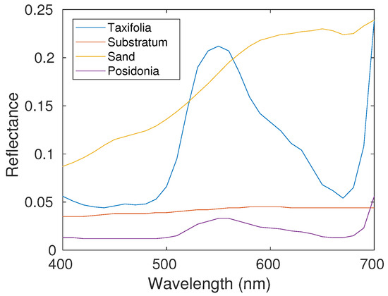
Figure 1. Real pure reflectance spectra: Caulerpa Taxifolia, substratum, sand and Posidonia. These spectra contain 31 spectral bands over the [400 nm, 700 nm] range.

We numerically generate the coefficients $a_{j,i}$ and $p_{n,i}$ of (6), so as to simulate relevant pure material “abundances”. To this end, we use the same protocol as in [50]. The considered images contain $100\times 24$ pixels and the maps of coefficients $a_{j,i}$ are shown in Figure 2. They are such that each pixel contains contributions from at least two pure materials, each of them having a maximum abundance of 80%. Moreover, the pure materials are distributed so as to have a spatial structure, with some materials more prominent in different regions (see Figure 2), which makes the considered images realistic.

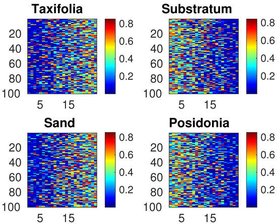
Figure 2. Maps of coefficients $a_{j,i}$ for all classes of pure materials (Caulerpa Taxifolia, substratum, sand and Posidonia). We numerically generated the coefficients $a_{j,i}$ and $p_{n,i}$ of (6), so as to simulate relevant pure material “abundances”. To this end, we used the same protocol as in [50]. The considered images contain $100\times 24$ pixels.

The $k_{1,i}$ and $k_{2,i}$ vectors of (6) were derived from the physical model of the OSOAA radiative transfer simulator [57]. These vectors depend on the considered water quality (clear or standard) and on the depth $d_i$ of the considered pixel i. We set these depths by creating a synthetic sea bottom profile, first defined by a reference depth $d_{ref}$ and where each pixel depth $d_i$ is randomly and uniformly drawn in an interval ranging from $-\mathsf{\Delta }$ to $+\mathsf{\Delta }$ around depth $d_{ref}$. The vectors $k_1$ and $k_2$ were first computed by the OSOAA software only for depths equal to 1, 2, 3, 4, 5 and 10 m. For any considered sea profile, these results from OSOAA were then used to derive the values of $k_{1,i}$ and $k_{2,i}$ for any depth $d_i$ of a pixel i of the considered scene. To this end, the following linear interpolation was used:

$$\begin{array}{ccc}\hfill k_{1,i}& =& \hfill (0.5-\alpha )k_1\left(d_i^{-}\right)+(0.5+\alpha )k_1\left(d_i^{+}\right)\hfill \end{array}$$

(13)

$$\begin{array}{ccc}\hfill k_{2,i}& =& \hfill (0.5-\alpha )k_2\left(d_i^{-}\right)+(0.5+\alpha )k_2\left(d_i^{+}\right)\hfill \end{array}$$

(14)

where $d_i^{-}$ and $d_i^{+}$ are the pixel-dependent closest depths, respectively, below and above $d_i$, for which OSOAA results are available (i.e., 1, 2, 3, 4, 5 and 10 m, as stated above). Moreover, $\alpha$ depends on the considered value $d_i$ of the interpolation point, with respect to the reference points $d_i^{-}$ and $d_i^{+}$. Figure 3 and Figure 4, respectively, illustrate the variations in $k_{1,i}$ and $k_{2,i}$ with respect to wavelength for the reference depth $d_{ref}=1.5$ m, for depth variations over the considered scene defined by $\mathsf{\Delta }=0.05$ m and for clear water.

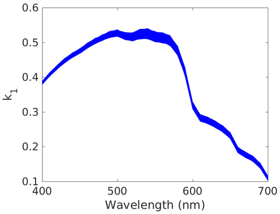
Figure 3. Variations in $k_{1,i}$ vs. wavelength, for all image pixels (one plot per pixel). Conditions: reference depth $d_{ref}=1.5$ m, depth variations over considered scene defined by $\mathsf{\Delta }=0.05$ m, clear water. The $k_{1,i}$ and $k_{2,i}$ vectors of (6) were derived from the physical model of the OSOAA radiative transfer simulator [57]. These vectors depend on the considered water quality (clear or standard) and on the depth $d_i$ of the considered pixel i.

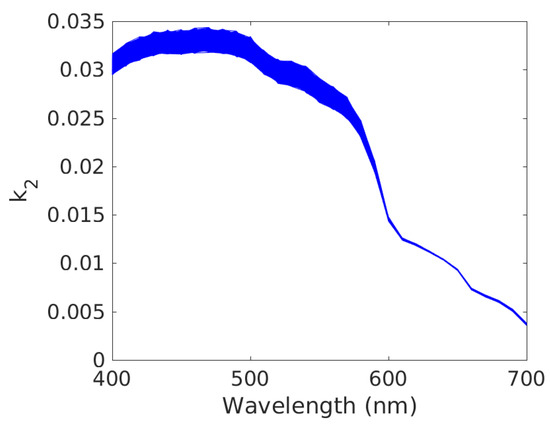
Figure 4. Variations in $k_{2,i}$ vs. wavelength, for all image pixels (one plot per pixel). Conditions: reference depth $d_{ref}=1.5$ m, depth variations over considered scene defined by $\mathsf{\Delta }=0.05$ m, clear water. The $k_{1,i}$ and $k_{2,i}$ vectors of (6) were derived from the physical model of the OSOAA radiative transfer simulator [57]. These vectors depend on the considered water quality (clear or standard) and on the depth $d_i$ of the considered pixel i.

Figure 5, Figure 6, Figure 7 and Figure 8 show the contributions ${\rho }_{i,j}$, defined by (8), within all mixed spectra $x_i$. Each of these figures corresponds to a given class j of pure materials and to all pixels i.

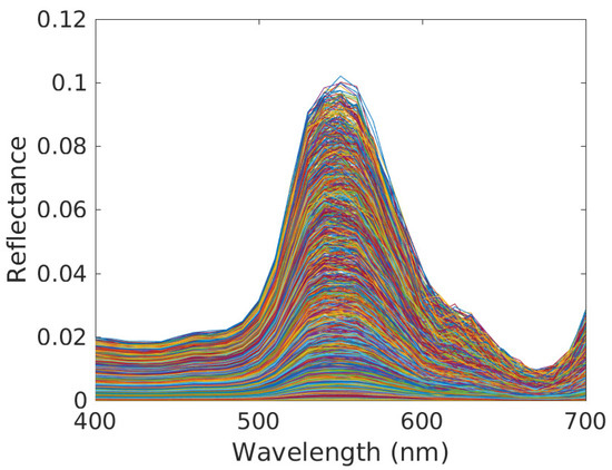
Figure 5. Contributions ${\rho }_{i,j}$ of Caulerpa taxifolia in the mixed reflectance spectra corresponding to all pixels (see (8), one plot per pixel). Conditions: clear water, reference depth $d_{ref}=1.5$ m and depth variations over considered scene defined by $\mathsf{\Delta }=0.25$ m.

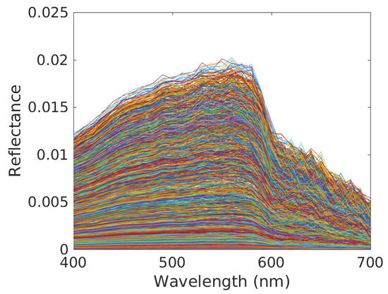
Figure 6. Contributions ${\rho }_{i,j}$ of substratum in the mixed reflectance spectra corresponding to all pixels (see (8), one plot per pixel). Conditions: clear water, reference depth $d_{ref}=1.5$ m and depth variations over considered scene defined by $\mathsf{\Delta }=0.25$ m.

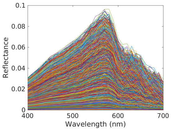
Figure 7. Contributions ${\rho }_{i,j}$ of sand in the mixed reflectance spectra corresponding to all pixels (see (8), one plot per pixel). Conditions: clear water, reference depth $d_{ref}=1.5$ m and depth variations over considered scene defined by $\mathsf{\Delta }=0.25$ m.

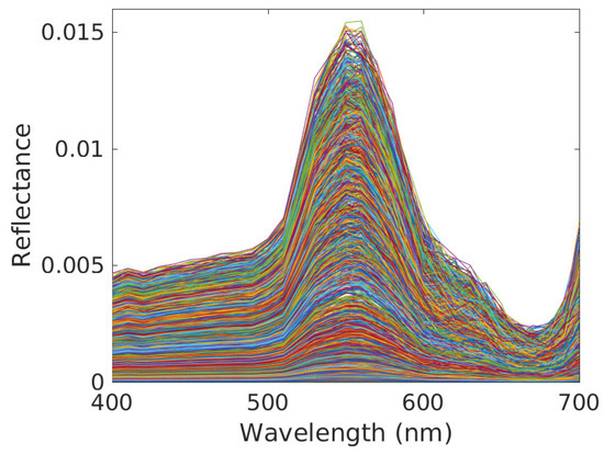
Figure 8. Contributions ${\rho }_{i,j}$ of Posidonia in the mixed reflectance spectra corresponding to all pixels (see (8), one plot per pixel). Conditions: clear water, reference depth $d_{ref}=1.5$ m and depth variations over considered scene defined by $\mathsf{\Delta }=0.25$ m.

4.2. Performance Criteria

Let us first consider the case where the measured data actually obey the model (9). Then, for each pixel i and each pure material j, the tested IP-NMF method yields a spectrum $e_{i,j}$ that estimates the pure spectrum $r_{i,j}$ of (9) but only up to a scale factor, as stated in Section 3: this scale indeterminacy is intrinsic to the mixing model (9) with spectral variability and very common in blind source separation/unsupervised unmixing problems, apart from the simplest remote sensing configuration defined in Section 1. This estimated spectrum $e_{i,j}$ should therefore be compared in terms of vector direction, not of magnitude, with its target value, which is $r_{i,j}$.

Now, consider mixed data defined by the model (7) and (8). Here, again, a comparison in terms of vector directions should be performed, but now between the result $e_{i,j}$ of IP-NMF and the actual contribution of pure material j in the observed spectrum (7) for pixel i, i.e., ${\rho }_{i,j}$. The spectra $e_{i,j}$ and ${\rho }_{i,j}$ are therefore compared by computing their Spectral Angle Mapper (SAM) [58] (we again stress that we only consider the directions of the vectors $e_{i,j}$ and ${\rho }_{i,j}$, and hence their SAM, so that this analysis does not depend on associated scale factors, such as the coefficients $c_{i,j}$ that appear in (9)). This SAM is then averaged over all pure materials and all pixels, thus yielding a unique performance figure for the complete image. This procedure is repeated for several runs (5 runs in the tests reported below), with different randomly drawn pixel depths. The mean of SAM over these runs is denoted as SAM(IP-NMF). As a comparison, we also compute the overall SAM, denoted as SAM(VCA), obtained when processing these data with the classical VCA method [54], which does not take spectral variability into account. Starting from the above overall SAM values of both considered methods, the percentage of improvement in SAM for our IP-NMF method, with respect to VCA, is then derived by computing

$$\frac{\mathrm{SAM}\left(\mathrm{VCA}\right)-\mathrm{SAM}\left(\text{IP-NMF}\right)}{\mathrm{SAM}\left(\text{IP-NMF}\right)}.$$

(15)

5. Test Results and Discussion

The above-defined protocol was applied to different water qualities and to various values of $d_{ref}$, $\mathsf{\Delta }$ and of the inertia penalty coefficient $\mu$ of the cost function (12), to analyze the performance in a variety of configurations. The results thus obtained are provided in the following subsections. Each of these subsections corresponds to a given type of water and a given value of $d_{ref}$, whereas $\mathsf{\Delta }$ and $\mu$ are varied. Three cases are thus considered for the type of water and value of $d_{ref}$, with increasing complexity.

5.1. Results for Clear Shallow Water

As a first step, we here investigate the case when the water is clear [48] and the reference depth of the scene is set to $d_{ref}=1.5$ m. In these conditions, various tests showed that IP-NMF has very low sensitivity with respect to the value of $\mu$ and that the optimum value (This optimum value was confirmed by other tests, performed with $d_{ref}=3.5$ m and standard-quality water) of $\mu$ most often ranges from 150 to 200 (IP-NMF is therefore more efficient with these values of $\mu$ than its version corresponding to $\mu =0$, i.e., UP-NMF). As an example, the variations in the overall SAM of our IP-NMF method, with respect to $\mu$ and for $\mathsf{\Delta }=0.25$ m, are shown in Table 1. The results reported in this and subsequent sections were therefore obtained when the parameter $\mu$ of the IP-NMF method was set to 150, and by performing 400 iterations with this method.

Table 1. Overall SAM, in degrees, of our IP-NMF method, versus its parameter $\mu$. Conditions: clear water, reference depth $d_{ref}=1.5$ m (i.e., shallow water), depth variations over considered scene defined by $\mathsf{\Delta }=0.25$ m.

$\mathit{\mu }$	SAM of IP-NMF (°)
25	4.30
50	4.26
75	4.22
100	4.20
125	4.17
150	4.15
175	4.13
200	4.13

In the above conditions, five values were considered for the magnitude $\mathsf{\Delta }$ of pixel-depth variations around $d_{ref}$. The corresponding results are shown in Table 2 and lead to the following conclusions. Our IP-NMF method always yields better performance than VCA and, when the magnitude $\mathsf{\Delta }$ of depth variations and hence the variability increase, i.e., when conditions become more difficult, the percentage of improvement in SAM for our IP-NMF method, with respect to VCA, monotonically increases, up to 14% for $\mathsf{\Delta }=0.25$ m. This confirms the better ability of IP-NMF to take into account the spectral variability induced by a non-constant sea depth.

Table 2. (a) Overall SAM, in degrees, of our IP-NMF method and of VCA, versus magnitude $\mathsf{\Delta }$ of pixel-depth variations around reference depth $d_{ref}$. (b) % of improvement in SAM of IP-NMF, as compared with SAM of VCA. Conditions: clear water, $d_{ref}=1.5$ m.

Δ (m)	SAM of IP-NMF	SAM of VCA	% of Improvement
0.05	4.30	4.58	6.5
0.10	3.90	4.19	7.4
0.15	4.13	4.52	9.4
0.20	3.96	4.34	9.6
0.25	4.15	4.73	14.0

The results obtained in this first configuration are made more explicit by displaying the pure material spectra estimates $e_{i,j}$ separately obtained by IP-NMF in each image pixel i, for each class j of materials. The spectra obtained for the highest considered value of $\mathsf{\Delta }$, namely $\mathsf{\Delta }=0.25$ m, are provided in Figure 9, Figure 10, Figure 11 and Figure 12. This shows that the shapes of these estimated spectra $e_{i,j}$ are similar to those of the components ${\rho }_{i,j}$ shown in Figure 5, Figure 6, Figure 7 and Figure 8. This is consistent with the discussion provided in Section 4.2, since the spectra $e_{i,j}$ estimate the components ${\rho }_{i,j}$ up to scale factors. Moreover, the actual components ${\rho }_{i,j}$ of any given class j of pure materials have significantly different magnitudes from one pixel to the other, as shown by the wide envelope of the plots of these pixel-dependent spectra in any of Figure 5, Figure 6, Figure 7 and Figure 8. In contrast, the freedom of the scale factors of the estimated spectra $e_{i,j}$ (corresponding to $c_{i,j}$ in (9)) is used by the IP-NMF method in order to obtain these spectra with relatively similar scales, as explained in Section 3 (see the inertia, i.e., spread, terms in the cost function). The envelope of the plots in any of Figure 9, Figure 10, Figure 11 and Figure 12 is thus narrow, and this is not an issue for the tests that we performed: only the shapes of these spectra should be taken into account.

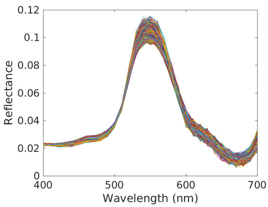
Figure 9. Pure material spectra estimates $e_{i,j}$ for Caulerpa taxifolia and all pixels (one plot per pixel). Conditions: clear water, reference depth $d_{ref}=1.5$ m (i.e., shallow water) and depth variations over considered scene defined by $\mathsf{\Delta }=0.25$ m (highest considered value). The parameter $\mu$ of the IP-NMF method was set to 150 and we performed 400 iterations with this method.

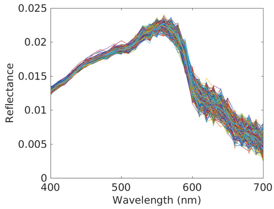
Figure 10. Pure material spectra estimates $e_{i,j}$ for substratum and all pixels (one plot per pixel). Conditions: clear water, reference depth $d_{ref}=1.5$ m (i.e., shallow water) and depth variations over considered scene defined by $\mathsf{\Delta }=0.25$ m (highest considered value).The parameter $\mu$ of the IP-NMF method was set to 150 and we performed 400 iterations with this method.

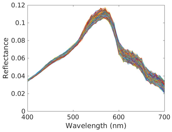
Figure 11. Pure material spectra estimates $e_{i,j}$ for sand and all pixels (one plot per pixel). Conditions: clear water, reference depth $d_{ref}=1.5$ m (i.e., shallow water) and depth variations over considered scene defined by $\mathsf{\Delta }=0.25$ m (highest considered value). The parameter $\mu$ of the IP-NMF method was set to 150 and we performed 400 iterations with this method.

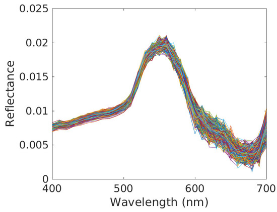
Figure 12. Pure material spectra estimates $e_{i,j}$ for Posidonia and all pixels (one plot per pixel). Conditions: clear water, reference depth $d_{ref}=1.5$ m (i.e., shallow water) and depth variations over considered scene defined by $\mathsf{\Delta }=0.25$ m (highest considered value). The parameter $\mu$ of the IP-NMF method was set to 150 and we performed 400 iterations with this method.

5.2. Results for Standard-Quality Shallow Water

We now consider the case when the reference depth of the scene is still set to $d_{ref}=1.5$ m, but we address a standard water quality [48]. The variations in the performance of IP-NMF and VCA with respect to $\mathsf{\Delta }$ are shown in Table 3. Here, again, IP-NMF always yields better performance than VCA. In most cases, the percentage of improvement in SAM for our IP-NMF method, with respect to VCA, monotonically increases with $\mathsf{\Delta }$ and is higher than for the corresponding case with clear water. Its maximum value is here higher than 18%.

Table 3. (a) Overall SAM, in degrees, of our IP-NMF method and of VCA, versus magnitude $\mathsf{\Delta }$ of pixel-depth variations around reference depth $d_{ref}$. (b) % of improvement in SAM of IP-NMF, as compared with SAM of VCA. Conditions: standard-quality water, $d_{ref}=1.5$ m.

Δ (m)	SAM of IP-NMF	SAM of VCA	% of Improvement
0.05	3.75	3.83	2.1
0.10	3.02	3.28	8.6
0.15	3.59	4.02	12.0
0.20	3.90	4.61	18.2
0.25	5.54	6.53	17.9

5.3. Results for Clear Deep Water

We eventually investigated the influence of the reference depth of the scene, by considering the much more difficult case in which it is set to $d_{ref}=7.5$ m, whereas we keep clear water, as in the first case (we here consider clear water because, for this water depth, the sea bottom is almost not visible for standard water). The variations in the performance of IP-NMF and VCA with respect to $\mathsf{\Delta }$ are shown in Table 4. Here, again, IP-NMF always yields better performance than VCA and the percentage of improvement in SAM for our IP-NMF method, with respect to VCA, often increases with $\mathsf{\Delta }$. That percentage of improvement is somewhat lower in this difficult case than in the previous two, but still significant: up to more than 8%.

Table 4. (a) Overall SAM, in degrees, of our IP-NMF method and of VCA, versus magnitude $\mathsf{\Delta }$ of pixel-depth variations around reference depth $d_{ref}$. (b) % of improvement in SAM of IP-NMF, as compared with SAM of VCA. Conditions: clear water, $d_{ref}=7.5$ m.

Δ (m)	SAM of IP-NMF	SAM of VCA	% of Improvement
0.05	3.97	4.03	1.5
0.10	4.75	4.82	1.5
0.15	5.00	5.18	3.6
0.20	5.32	5.75	8.1
0.25	7.00	7.44	6.3

The SAM of IP-NMF is here significantly higher than in the previous two cases: for the same range of values of $\mathsf{\Delta }$, it here increases up to $7.{00}^{\circ }$, as compared with the maximum values $4.{15}^{\circ }$ and $5.{54}^{\circ }$ obtained in the previous two cases. One may relate these values to the fact that the SAM-based classification method available in the commercial ENVI software, version 2019, [59] considers that spectra from a class have a SAM lower than $0.1\mathrm{rad}\simeq 5.{73}^{\circ }$, with respect to the representative of that class. Therefore, for the maximum value $\mathsf{\Delta }=0.25$ m, IP-NMF can hardly separate the considered classes of materials for the low signal magnitude faced in the difficult conditions considered in the present section. For the water depth variability defined by $\mathsf{\Delta }=0.25$ m, IP-NMF is therefore of main interest for moderately deep water. However, when considering $\mathsf{\Delta }\le 0.2$ m, IP-NMF remains satisfactory even in the difficult conditions considered here, since the maximum SAM is then $5.{32}^{\circ }$, which is compatible with the $5.{73}^{\circ }$ bound of the ENVI software. Moreover, the magnitude of $\mathsf{\Delta }$ may be decreased by splitting the overall scene into subscenes, as explained in Section 2.2 and hereafter.

6. Conclusions

The first contribution in this paper consists of an analysis of the specific hyperspectral mixing model that we recently introduced for the sea bottom. We analytically showed that such data can be processed with blind unmixing methods designed to handle spectral variability and we defined such a method. We then developed a detailed framework to numerically create realistic ocean remote sensing data. We used it to assess the performance of the proposed approach, by comparing the estimated spectra provided by our unmixing method to the ground truth that was here available thanks to our numerical framework. It should be noted that, in contrast, applying our method to real data would be of interest but would not allow one to perform the above-mentioned detailed performance assessment. This results from the fact that such an analysis requires a ground truth consisting of a different spectrum for each type of pure material and each pixel, due to spectral variability, and this cannot be built in practice for a reasonable number of pixels. Nonetheless, in our realistic numerical framework, the proposed method always outperforms the considered method from the literature and is able to distinguish various classes of oceanic pure materials even in difficult conditions—for instance, for reference water depths up to 7.5 m if pixel depths vary up to $\pm 0.2$ m around that reference. Moreover, as explained in Section 2.2, the overall scene may be first segmented, in order to obtain smaller depth variations over each subscene and thus to ensure that, for instance, these variations do not exceed the above-mentioned $\pm 0.2$ m range. Our unmixing method may then be successfully applied separately over each subscene.

This investigation therefore confirms that, for complex observed oceanic scenes, the data model that we recently introduced allows one to develop associated unmixing methods that yield better performance than unmixing methods from the literature intended for the standard mixing model. Thus far, we have developed two complementary methods for our data model. The method of [50] exploits the entire structure of our model but is supervised (i.e., non-blind), since it requires one to know (or to previously estimate) some of the parameters of the model, which is constraining. In contrast, the new method proposed in the present paper is unsupervised and therefore more attractive, but it only exploits part of the structure of the considered data model, by reformulating it so as to insert it into the more general class of models with intraclass variability and by then processing the data with a generic method intended for intraclass variability. This therefore opens the way to future investigations, where we will aim at developing a third type of method that combines the attractive features of the above two, i.e., that operates in an unsupervised way and that exploits all the structure of the considered specific data model, by estimating all its parameters. One may expect to thus achieve better unmixing performance for data that obey the considered model.

References

- Bioucas-Dias, J.M.; Plaza, A.; Dobigeon, N.; Parente, M.; Du, Q.; Gader, P.; Chanussot, J. Hyperspectral unmixing overview: Geometrical, statistical, and sparse regression-based approaches. IEEE J. Sel. Top. Appl. Earth Obs. Remote Sens. 2012, 5, 354–379. [Google Scholar] [CrossRef]
- Keshava, N.; Mustard, J.F. Spectral unmixing. IEEE Signal Process. Mag. 2002, 19, 44–57. [Google Scholar] [CrossRef]
- Deville, Y.; Duarte, L.T.; Hosseini, S. Nonlinear Blind Source Separation and Blind Mixture Identification. METHODS for Bilinear, Linear-Quadratic and Polynomial Mixtures; Springer Briefs in Electrical and Computer Engineering, Springer Nature; Springer: Berlin/Heidelberg, Germany, 2021. [Google Scholar] [CrossRef]
- Meganem, I.; Déliot, P.; Briottet, X.; Deville, Y.; Hosseini, S. Linear-quadratic mixing model for reflectances in urban environments. IEEE Trans. Geosci. Remote Sens. 2014, 52, 544–558. [Google Scholar] [CrossRef]
- Deville, Y.; Duarte, L.T. An overview of blind source separation methods for linear-quadratic and post-nonlinear mixtures. In Proceedings of the 12th International Conference on Latent Variable Analysis and Signal Separation (LVA/ICA 2015), Liberec, Czech Republic, 25–28 August 2015; LNCS 9237. Springer International Publishing: Cham, Switzerland, 2015; pp. 155–167. [Google Scholar]
- Deville, Y.; Hosseini, S. Blind source separation methods based on output nonlinear correlation for bilinear mixtures of an arbitrary number of possibly correlated signals. In Proceedings of the Eleventh IEEE Sensor Array and Multichannel Signal Processing Workshop (SAM 2020), Hangzhou, China, 8–11 June 2020. [Google Scholar]
- Meganem, I.; Deville, Y.; Hosseini, S.; Déliot, P.; Briottet, X.; Duarte, L.T. Linear-quadratic and polynomial Non-negative Matrix Factorization; application to spectral unmixing. In Proceedings of the 19th European Signal Processing Conference (EUSIPCO 2011), Barcelona, Spain, 29 August–2 September 2011. [Google Scholar]
- Benhalouche, F.Z.; Deville, Y.; Karoui, M.S.; Ouamri, A. Hyperspectral endmember spectra extraction based on constrained linear-quadratic matrix factorization using a projected gradient method. In Proceedings of the 2016 IEEE International Workshop on Machine Learning for Signal Processing (MLSP 2016), Salerno, Italy, 13–16 September 2016; pp. 1–6. [Google Scholar]
- Benhalouche, F.Z.; Karoui, M.S.; Deville, Y. Linear-quadratic NMF-based urban hyperspectral data unmixing with some known endmembers. In Proceedings of the 9th Workshop on Hyperspectral Image and Signal Processing: Evolution in Remote Sensing (WHISPERS 2018), Amsterdam, The Netherlands, 23–26 September 2018. [Google Scholar]
- Benhalouche, F.Z.; Deville, Y.; Karoui, M.S.; Ouamri, A. Hyperspectral unmixing based on constrained bilinear or linear-quadratic matrix factorization. Remote Sens. 2021, 13, 2132. [Google Scholar] [CrossRef]
- Benkouider, Y.K.; Benhalouche, F.Z.; Karoui, M.S.; Deville, Y.; Hosseini, S. Bilinear matrix factorization using a gradient method for unmixing hyperspectral images combined with multispectral data. In Proceedings of the 9th Workshop on Hyperspectral Image and Signal Processing: Evolution in Remote Sensing (WHISPERS 2018), Amsterdam, The Netherlands, 23–26 September 2018. [Google Scholar]
- Deville, Y. From separability/identifiability properties of bilinear and linear-quadratic mixture matrix factorization to factorization algorithms. Digit. Signal Process. 2019, 87, 21–33. [Google Scholar] [CrossRef]
- Eches, O.; Guillaume, M. A bilinear-bilinear nonnegative matrix factorization method for hyperspectral unmixing. IEEE Geosci. Remote Sens. Lett. 2014, 11, 778–782. [Google Scholar] [CrossRef]
- Guerrero, A.; Deville, Y.; Hosseini, S. A blind source separation method based on output nonlinear correlation for bilinear mixtures. In Proceedings of the 14th International Conference on Latent Variable Analysis and Signal Separation (LVA/ICA 2018), Guildford, UK, 2–5 July 2018; Part of Springer Nature 2018, LNCS 10891. Springer International Publishing AG: Cham, Switzerland, 2018; pp. 183–192. [Google Scholar]
- Huard, P.; Marion, R. Study of non-linear mixing in hyperspectral imagery—A first attempt in the laboratory. In Proceedings of the Third Workshop on Hyperspectral Image and Signal Processing: Evolution in Remote Sensing (WHISPERS 2011), Lisbon, Portugal, 6–9 June 2011. [Google Scholar]
- Jarboui, L.; Hosseini, S.; Deville, Y.; Guidara, R.; Hamida, A.B. A new unsupervised method for hyperspectral image unmixing using a linear-quadratic model. In Proceedings of the First International Conference of Advanced Technologies for Signal and Image Processing (ATSIP 2014), Sousse, Tunisia, 17–19 March 2014; pp. 423–428. [Google Scholar]
- Jarboui, L.; Hosseini, S.; Guidara, R.; Deville, Y.; Hamida, A.B. A MAP-based NMF approach to hyperspectral image unmixing using a linear-quadratic mixture model. In Proceedings of the 2016 IEEE International Conference on Acoustics, Speech, and Signal Processing (ICASSP 2016), Shanghai, China, 20–25 March 2016; pp. 3356–3360. [Google Scholar]
- Meganem, I.; Déliot, P.; Briottet, X.; Deville, Y.; Hosseini, S. Physical modelling and non-linear unmixing method for urban hyperspectral images. In Proceedings of the Third Workshop on Hyperspectral Image and Signal Processing (WHISPERS 2011), Lisbon, Portugal, 6–9 June 2011. [Google Scholar]
- Meganem, I.; Deville, Y.; Hosseini, S.; Déliot, P.; Briottet, X. Linear-quadratic blind source separation Using NMF to unmix urban hyperspectral images. IEEE Trans. Signal Process. 2014, 62, 1822–1833. [Google Scholar] [CrossRef]
- Sigurdsson, J.; Ulfarsson, M.O.; Sveinsson, J.R. Blind nonlinear hyperspectral unmixing using an lq regularizer. In Proceedings of the 2018 IEEE International Geoscience and Remote Sensing Symposium (IGARSS 2018), Valencia, Spain, 22–27 July 2018; pp. 4229–4232. [Google Scholar]
- Su, Y.; Li, J.; Qi, H.; Gamba, P.; Plaza, A.; Plaza, J. Multi-task learning with low-rank matrix factorization for hyperspectral nonlinear unmixing. In Proceedings of the 2019 IEEE International Geoscience and Remote Sensing Symposium (IGARSS 2019), Yokohama, Japan, 28 July–2 August 2019; pp. 2127–2130. [Google Scholar]
- Deville, Y.; Revel, C.; Achard, V.; Briottet, X. Application and extension of PCA concepts to blind unmixing of hyperspectral data with intra-class variability. In Advances in Principal Component Analysis—Research and Development; Naik, G.R., Ed.; Springer: Singapore, 2018; pp. 225–252. [Google Scholar]
- Revel, C.; Deville, Y.; Achard, V.; Briottet, X.; Weber, C. Inertia-constrained pixel-by-pixel nonnegative matrix factorisation: A hyperspectral unmixing method dealing with intra-class variability. Remote Sens. 2018, 10, 170. [Google Scholar] [CrossRef]
- Borsoi, R.A.; Imbiriba, T.; Bermudez, J.C.M.; Richard, C.; Chanussot, J.; Drumetz, L.; Tourneret, J.-Y.; Zare, A.; Jutten, C. Spectral variability in hyperspectral data unmixing. A comprehensive review. IEEE Geosci. Remote Sens. Mag. 2021, 9, 223–270. [Google Scholar] [CrossRef]
- Zare, A.; Ho, K.C. Endmember variability in hyperspectral analysis. IEEE Signal Process. Mag. 2014, 31, 95–104. [Google Scholar] [CrossRef]
- Cheng, Y.; Zhao, L.; Chen, S.; Li, X. Hyperspectral unmixing network accounting for spectral variability based on a modified scaled and a perturbed linear mixing model. Remote Sens. 2023, 15, 3890. [Google Scholar] [CrossRef]
- Imbiriba, T.; Borsoi, R.A.; Bermudez, J.C.M. Generalized linear mixing model accounting for endmember variability. In Proceedings of the 2018 IEEE International Conference on Acoustics, Speech and Signal Processing (ICASSP 2018), Calgary, AB, Canada, 15–20 April 2018; pp. 1862–1866. [Google Scholar]
- Brezini, S.E.; Deville, Y.; Karoui, M.S.; Benhalouche, F.Z.; Ouamri, A. A penalization-based NMF approach for hyperspectral unmixing addressing spectral variability with an additively-tuned mixing model. In Proceedings of the 2021 IEEE International Geoscience and Remote Sensing Symposium (IGARSS 2021), Brussels, Belgium, 11–16 July 2021; pp. 3841–3844. [Google Scholar]
- Azar, S.G.; Meshgini, S.; Beheshti, S.; Rezaii, T.Y. Linear mixing model with scaled bundle dictionary for hyperspectral unmixing with spectral variability. Signal Process. 2021, 188, 108214. [Google Scholar] [CrossRef]
- Benhalouche, F.Z.; Karoui, M.S.; Deville, Y. Gradient-based NMF methods for hyperspectral unmixing addressing spectral variability with a multiplicative-tuning linear mixing model. In Proceedings of the 2021 IEEE International Geoscience and Remote Sensing Symposium (IGARSS 2021), Brussels, Belgium, 11–16 July 2021; pp. 3205–3208. [Google Scholar]
- Deville, Y.; Faury, G.; Achard, V.; Briottet, X. An NMF-based method for jointly handling mixture nonlinearity and intraclass variability in hyperspectral blind source separation. Digit. Signal Process. 2023, 133, 103838. [Google Scholar] [CrossRef]
- Drumetz, L.; Veganzones, M.A.; Henrot, S.; Phlypo, R.; Chanussot, J.; Jutten, C. Blind hyperspectral unmixing using an extended linear mixing model to address spectral variability. IEEE Trans. Image Process. 2016, 25, 3890–3905. [Google Scholar] [CrossRef] [PubMed]
- Hong, D.; Zhu, X.X. SULoRA: Subspace unmixing with low-rank attribute embedding for hyperspectral data analysis. IEEE J. Sel. Top. Signal Process. 2018, 12, 1351–1363. [Google Scholar] [CrossRef]
- Hong, D.; Yokoya, N.; Chanussot, J.; Zhu, X.X. An augmented linear mixing model to address spectral variability for hyperspectral unmixing. IEEE Trans. Image Process. 2019, 28, 1923–1938. [Google Scholar] [CrossRef]
- Karoui, M.S.; Benhalouche, F.Z.; Deville, Y. Hyperspectral unmixing with a modified augmented linear mixing model addressing spectral variability. In Proceedings of the 2022 IEEE Mediterranean and Middle-East Geoscience and Remote Sensing Symposium (M2GARSS 2022), Istanbul, Turkey, 7–9 March 2022; pp. 66–69. [Google Scholar]
- Liu, H.; Lu, Y.; Wu, Z.; Du, Q.; Chanussot, J.; Wei, Z. Bayesian unmixing of hyperspectral image sequence with composite priors for abundance and endmember variability. IEEE Trans. Geosci. Remote Sens. 2022, 60, 5503515. [Google Scholar] [CrossRef]
- Ren, L.; Hong, D.; Gao, L.; Sun, X.; Huang, M.; Chanussot, J. Orthogonal subspace unmixing to address spectral variability for hyperspectral image. IEEE Trans. Geosci. Remote Sens. 2023, 61, 5501713. [Google Scholar] [CrossRef]
- Sahadevan, A.S.; Ahmad, T.; Lyngdoh, R.B.; Kumar, D.N. Endmember variability based abundance estimation of red and black soil over sparsely vegetated area using AVIRIS-NG hyperspectral image. Adv. Space Res. 2023; in press. [Google Scholar] [CrossRef]
- Salehani, Y.E.; Arabnejad, E.; Gazor, S. Augmented Gaussian linear mixture model for spectral variability in hyperspectral unmixing. In Proceedings of the 2021 IEEE International Conference on Acoustics, Speech and Signal Processing (ICASSP 2021), Toronto, ON, Canada, 6–11 June 2021; pp. 1880–1884. [Google Scholar]
- Shi, S.; Zhao, M.; Zhang, L.; Chen, J. Variational autoencoders for hyperspectral unmixing with endmember variability. In Proceedings of the 2021 IEEE International Conference on Acoustics, Speech and Signal Processing (ICASSP 2021), Toronto, ON, Canada, 6–11 June 2021; pp. 1875–1879. [Google Scholar]
- Su, L.; Liu, J.; Yuan, Y.; Chen, Q. A multi-attention autoencoder for hyperspectral unmixing based on the extended linear mixing model. Remote Sens. 2023, 15, 2898. [Google Scholar] [CrossRef]
- Thouvenin, P.A.; Dobigeon, N.; Tourneret, J.Y. Hyperspectral unmixing with spectral variability using a perturbed linear mixing model. IEEE Trans. Signal Process. 2016, 64, 525–538. [Google Scholar] [CrossRef]
- Xu, M.; Zou, X.; Liu, S.; Sheng, H.; Yang, Z. Manifold regularized sparse archetype analysis considering endmember variability. IEEE Geosci. Remote Sens. Lett. 2023, 20, 5506805. [Google Scholar]
- Yu, J.; Wang, B.; Lin, Y.; Li, F.; Cai, J. A novel inequality-constrained weighted linear mixture model for endmember variability. Remote Sens. Environ. 2021, 257, 112359. [Google Scholar] [CrossRef]
- Zhang, G.; Mei, S.; Xie, B.; Feng, Y.; Du, Q. Spectral variability augmented two-stream network for hyperspectral sparse unmixing. IEEE Geosci. Remote. Sens. Lett. 2022, 19, 6014605. [Google Scholar] [CrossRef]
- Zhao, M.; Shi, S.; Chen, J.; Dobigeon, N. A 3-D-CNN framework for hyperspectral unmixing with spectral variability. IEEE Trans. Geosci. Remote. Sens. 2022, 60, 5521914. [Google Scholar] [CrossRef]
- Karoui, M.S.; Benhalouche, F.Z.; Deville, Y. A gradient-based method for the modified augmented linear mixing model addressing spectral variability for hyperspectral unmixing. In Proceedings of the 2022 IEEE International Geoscience and Remote Sensing Symposium (IGARSS 2022), Kuala Lumpur, Malaysia, 17–22 July 2022; pp. 3279–3282. [Google Scholar]
- Chami, M.; Lenot, X.; Guillaume, M.; Lafrance, B.; Briottet, X.; Minghelli, A.; Jay, S.; Deville, Y.; Serfaty, V. Analysis and quantification of seabed adjacency effects in the subsurface upward radiance in shallow waters. Opt. Express 2019, 27, A319–A338. [Google Scholar] [CrossRef]
- Wang, X.; Zhong, Y.; Zhang, L.; Xu, Y. Blind hyperspectral unmixing considering the adjacency effect. IEEE Trans. Geosci. Remote Sens. 2019, 57, 6633–6649. [Google Scholar] [CrossRef]
- Guillaume, M.; Juste, L.; Lenot, X.; Deville, Y.; Lafrance, B.; Chami, M.; Jay, S.; Minghelli, A.; Briottet, X.; Serfaty, V. NMF hyperspectral unmixing of the sea bottom: Influence of the adjacency effects, model and method. In Proceedings of the WHISPERS 2018, Amsterdam, The Netherlands, 23–26 September 2018. [Google Scholar]
- Deville, Y.; Brezini, S.E.; Benhalouche, F.Z.; Karoui, M.S.; Guillaume, M.; Lenot, X.; Lafrance, B.; Chami, M.; Jay, S.; Minghelli, A.; et al. Hyperspectral oceanic remote sensing with adjacency effects: From spectral-variability-based modeling to performance of associated blind unmixing methods. In Proceedings of the 2019 IEEE International Geoscience and Remote Sensing Symposium (IGARSS 2019), Yokohama, Japan, 28 July–2 August 2019; pp. 282–285. [Google Scholar]
- Cichocki, A.; Zdunek, R.; Phan, A.H.; Amari, S.-I. Nonnegative Matrix and Tensor Factorizations. Applications to Exploratory Multi-Way Data Analysis and Blind Source Separation; Wiley: Chichester, UK, 2009. [Google Scholar]
- Comon, P.; Jutten, C. (Eds.) Handbook of Blind Source Separation. Independent Component Analysis and Applications; Academic Press: Oxford, UK, 2010. [Google Scholar]
- Nascimento, J.M.P.; Dias, J.M.B. Vertex component analysis: A fast algorithm to unmix hyperspectral data. IEEE Trans. Geosci. Remote Sens. 2005, 43, 898–910. [Google Scholar] [CrossRef]
- Heinz, D.; Chang, C.-I. Fully constrained least squares linear spectral mixture analysis method for material quantification in hyperspectral imagery. IEEE Trans. Geosci. Remote Sens. 2001, 39, 529–545. [Google Scholar] [CrossRef]
- Lawson, C.L.; Hanson, R.J. Solving Least Squares Problems, SIAM’s Classics in Applied Mathematics; Prentice-Hall: Englewoods Cliffs, NJ, USA, 1995. [Google Scholar]
- Chami, M.; Lafrance, B.; Fougnie, B.; Chowdhary, J.; Harmel, T.; Waquet, F. OSOAA: A vector radiative transfer model of coupled atmosphere-ocean system for a rough sea surface application to the estimates of the directional variations of the water leaving reflectance to better process multi-angular satellite sensors data over the ocean. Opt. Express 2015, 23, 27829–27852. [Google Scholar] [CrossRef]
- Kruse, F.A.; Lefkoff, A.B.; Boardman, J.W.; Heidebrecht, K.B.; Shapiro, A.T.; Barloon, P.J.; Goetz, A.F.H. The spectral image processing system (SIPS)—Interactive visualization and analysis of imaging spectrometer data. Remote Sens. Environ. 1993, 44, 145–163. [Google Scholar] [CrossRef]
- L3HARRIS Geospatial, ENVI Software. Available online: https://www.l3harrisgeospatial.com/docs/spectralanglemapper.html (accessed on 1 February 2019).
Disclaimer/Publisher’s Note: The statements, opinions and data contained in all publications are solely those of the individual author(s) and contributor(s) and not of MDPI and/or the editor(s). MDPI and/or the editor(s) disclaim responsibility for any injury to people or property resulting from any ideas, methods, instructions or products referred to in the content. |
© 2023 by the authors. Licensee MDPI, Basel, Switzerland. This article is an open access article distributed under the terms and conditions of the Creative Commons Attribution (CC BY) license (https://creativecommons.org/licenses/by/4.0/).