Determination of Crop Coefficients and Evapotranspiration of Potato in a Semi-Arid Climate Using Canopy State Variables and Satellite-Based NDVI

Abstract

Estimating crop coefficients and evapotranspiration (ET) accurately is crucial for optimizing irrigation. Remote sensing techniques using green canopy cover, leaf area index (LAI), and normalized difference vegetation index (NDVI) have been applied to estimate basal crop coefficients (Kcb) and ET for different crops. However, analysis of the potential of these techniques to improve water management in irrigated potato (Solanum tuberosum L.) is still lacking. This study aimed to assess the modified nonlinear relationship between LAI, Kcb and NDVI in estimating crop coefficients (Kc) and ET of potato. Moreover, Kc and ET were derived from the measured fraction of green canopy cover (FGCC) and the FAO-56 approach. ET estimated from the FAO-56, FGCC and NDVI approaches were compared with the ET simulated using the LINTUL-Potato model. The results showed that the Kc values based on FGCC and NDVI were on average 0.16 lower than values based on FAO-56 Kc during the mid-season growing stage. ET estimated from FAO-56, FGCC and NDVI compared well with ET calculated by the LINTUL-Potato model, with RMSE values of 0.83, 0.79, and 0.78 mm day⁻¹, respectively. These results indicate that dynamic crop coefficients and potato ET can be estimated from canopy cover and NDVI. The outcomes of this study will assist potato growers in determining crop water requirements using real-time ETo, canopy state variables and NDVI data from satellite images.

1. Introduction

South Africa faces challenges of water scarcity and high competition for water, mainly due to an increasing human population, economic growth, climate change, and deteriorating water quality. The country has a semi-arid climate, with an average annual rainfall of approximately 500 mm [1]. This amount of rainfall is low for agricultural production, considering that the country is poorly endowed with groundwater resources and inland rivers [2]. Therefore, there is an urgent need to improve water productivity and reduce the non-beneficial use of water. This is particularly important for potato (Solanum tuberosum L.) growers, who depend on irrigation as dryland potato production is generally too risky [1].

Studies by Franke et al. [3] and Steyn et al. [4] assessed resource use efficiencies of potato production in the main growing regions of South Africa. The results of these studies indicate substantial variability in resource use efficiency, specifically water use efficiency (WUE), between growers within regions with relatively homogeneous agro-ecological conditions. The variation in WUE within regions was attributed to differences in tuber yield and irrigation amounts applied to potato due to a lack in the use of irrigation scheduling tools [5].

Various irrigation scheduling tools are available today, including soil-, plant-, and atmosphere-based methods [6,7]. Atmospheric scheduling methods rely on timely and accurate information on the amount of water lost by the crop, which is represented by evapotranspiration (ET) [8,9]. Maximum ET (ETmax) can be calculated as the product of a crop coefficient and the reference evapotranspiration (ETo) (ETmax = Eto ∗ Kc) [10]. ETo represents the meteorological evaporative demand and can be estimated using the FAO Penman-Monteith equation, which uses weather variables as inputs [10]. Actual ET is lower than ETmax under soil water limiting conditions [9].

Traditional methods for estimating crop coefficients involve field experiments using changes in soil water content and lysimeter measurements [8]. However, these methods are prone to large errors, mainly because point measurements are taken to represent the entire field, overlooking the inherent spatial variability of soil and plant characteristics within the field [10,11]. In addition, these methods are time-consuming and expensive.

Crop coefficients can be estimated using published curves and empirical equations, such as those published in FAO Irrigation Paper no. 56 [10]. However, crop coefficients based on FAO equations are often site-specific and cannot be relied upon for accurate crop ET estimations and irrigation scheduling [12]. Additionally, FAO-56 crop coefficients generally assume that crops are grown free of stress, which does not reflect reality. Therefore, there is a need to test new methods, such as those utilizing remote sensing, to estimate crop coefficients in real-time and accurately reflect the crop conditions at a specific developmental stage [8].

Remote sensing technology has been adopted to monitor crops and derive canopy reflectance-based crop coefficients that are used to estimate crop ET [13,14,15]. Remote sensing spectral vegetation indices (VIs), such as the normalized difference vegetation index (NDVI), soil-adjusted vegetation index (SAVI), and enhanced vegetation index (EVI) [16,17], have been widely studied and shown to have strong relationships with plant biophysical variables such as leaf area index (LAI), aboveground biomass, green canopy cover percentage (GCC), and chlorophyll content [11,18]. These biophysical variables are directly related to plant canopy processes, specifically ET, photosynthesis and primary productivity [13,19]. Researchers have used this knowledge to relate spectral VIs to single crop coefficient (Kc) and basal crop coefficient (Kcb) values for the estimation of crop water demand [11,20]. Jayanthi et al. [21] mentioned that estimating Kc values from remote sensing VIs is an effective approach compared to traditional methods, since the VIs reflect actual crop growth patterns as influenced by crop management, climate and soil factors. Remote sensing-based Kc and Kcb for crops, such as maize (Zea mays L.), soybean (Glycine max L.), potato, wheat (Triticum aestivum L.), lettuce (Lactuca sativa L.) and table grapes (Vitis vinifera L.), have been developed successfully [22,23]. Jayanthi et al. [21] related reflectance-based crop coefficients to SAVI and used a linear equation to estimate ET and soil water content in potato. Duchemin et al. [16] developed a linear relationship between NDVI and ET to facilitate irrigation management for wheat crops in Morrocco. Er–Raki et al. [22] developed a relationship between Kc and NDVI to estimate the ET of table grapes in the semi-arid regions of Northwest Mexico.

Although remote sensing has been used to derive Kc and Kcb for various crops in different environments, no such studies have been conducted to assess Kcb-VI relationships for irrigated potato under southern African growing conditions. Local calibration of remote-sensing-based crop coefficients is required to ensure accurate estimation of ET [16]. Furthermore, there is a lack of research on the use of nonlinear relationships between Kcb, LAI, GCC, and NDVI for potato, as proposed by Choudhury et al. [17] and later modified by Campos et al. [24]. The only study on the use of reflectance-based crop coefficients for potatoes was performed in Idaho, USA by Jayanthi et al. [21], and was based on a linear relationship combining the maximum and minimum values of SAVI obtained under the experimental conditions of their study, making it impractical to adopt the resultant linear equation to estimate Kcb for other production conditions. In addition, potato growers in southern Africa grow different varieties compared to those studied by Jayanthi et al. [21] (Russet Burbank and Norkotah), which justifies the need to establish the relationship between Kcb and canopy state variables for local potato varieties.

The objectives of this study were as follows:

• to assess the relationship between GCC, LAI, and NDVI for potato variety Mondial, under southern African production conditions;
• to evaluate the performance of the modified nonlinear relationship between Kcb and NDVI proposed by Choudhury et al. [17] and modified by Campos et al. [24] in estimating ET of potato;
• to estimate Kc and ET of potato based on FAO-56, the Kcb-fraction of GCC (FGCC) and the Kcb-NDVI approaches;
• to compare ET values from the above three approaches with ET simulated by the LINTUL-Potato model.

2. Materials and Methods

2.1. Study Area, Field Selection and Crop Management

The study was conducted on six commercial potato fields on six different farms in two production regions of South Africa. One field was in Gauteng Province nearby the town of Bapsfontein (26.0209°S, 28.4276°E). The five remaining fields were selected from five different farms near the village of Christiana in the Western Free State (WFS) Province (27.8847°S, 25.1533°E). Bapsfontein is characterized by a semi-arid climate with rainy and mildly hot summers (November to February), and dry and mildly cold winters (May to August). The WFS region is characterized by a semi-arid climate with hot and rainy summers as well as cold and dry winters. Summer seasonal rainfall for both regions ranges between 360 and 450 mm [25,26]. During summer, daily mean minimum temperatures range between 12 and 17 °C, and daily mean maximum temperatures range between 24 and 30 °C [25].

The field at Bapsfontein was monitored from August to December 2021, whereas fields in the WFS were monitored between November 2021 to March 2022. The mildly cold winters allow growers in Gauteng to start planting as early as August and harvest in December/January when potato prices are relatively high. All monitored fields were planted with the potato variety Mondial, which is the most widely grown potato variety in South Africa. For all monitored fields, potatoes were grown under center-pivot irrigation systems and crops were managed using advanced techniques. Less intensive monitoring was performed on the field at Bapsfontein (Field 1), which only consisted of collecting plant growth variables including, LAI, GCC, fraction of intercepted photosynthetically active radiation (FIPAR) and satellite-based NDVI (

Table 1. Field and crop management information, including field size, planting and harvest dates, vine kill-off date, monitoring intensity and amount of fertilizer applied (nitrogen N, phosphorus P and potassium K).

Field No.	Field Size (ha)	Planting Date	Vine Kill-Off Date	Monitoring	N-P-K (kg ha−1)
1	14	04-Aug-21	17-Nov-21	Less intensive	-
2	22	08-Nov-21	05-Mar-22	Intensive	302-160-291
3	18	05-Nov-21	10-Mar-22	Intensive	229-281-287
4	36	15-Nov-21	07-Mar-22	Intensive	316-160-300
5	32	11-Nov-21	02-Mar-22	Intensive	311-171-295
6	20	17-Nov-21	09-Mar-22	Intensive	322-138-311

). More intensive monitoring was carried out on all WFS fields (Field 2–6) and consisted of collecting information on weather variables, irrigation, soil analysis, plant growth variables, crop management information, drainage and final yield (Table 1). For Fields 2–6, the crops were grown on ridges. Mean interrow spacing was 0.9 m and the average spacing between plants was 0.3 m. The growers applied recommended nutrient rates (N, P, and K) (Table 1). Potatoes in all fields were mainly grown for seed, therefore, the vines were killed off chemically before full crop senescence.

2.2. Field Data Measurements

2.2.1. Weather Information

Daily weather data, including minimum and maximum temperature, relative humidity, solar radiation, wind speed, and rainfall, were recorded by automatic weather stations (AWS) installed at Fields 2 and 3. Tipping-bucket rain gauges were installed in each field in the WFS to record the amount of water supplied to the crops through rainfall and irrigation. Temperature data were used to calculate the growing degree days (GDD) from planting until vine killing using a base temperature (Tb) of 2 °C [27] (Equation (1)).

GDD = (T_max + T_min)/2 − Tb

(1)

where T_max is the daily maximum temperature and T_min is the daily minimum temperature.

2.2.2. Irrigation and Drainage

Irrigation of all monitored fields was managed by the respective growers without any intervention by the researchers. This meant that growers determined when and how much irrigation to apply per irrigation event. Irrigation (I) and drainage (D) were not measured for Field 1; therefore, Field 1 was left out in the subsequent Kc and ET calculations. Irrigation was measured only in the WFS (Fields 2–6) using pressure transducers and a transit-time ultrasonic flow meter. The pressure transducer recorded irrigation pressure every 10 min, which allowed to calculate the time of each irrigation event. An ultrasonic flow meter was used to measure water flow rate (m³ hr⁻¹) once during the cropping season. The amount of water for each irrigation event was then calculated as the product of the flow rate and irrigation time divided by the field area (Table 1). The coefficient of uniformity (CU) and application efficiency (AE) for all center pivots were determined and the latter was used to calculate the effective irrigation applied (

Table 2. Mean daily irrigation applied (I), coefficient of uniformity (CU) and application efficiency (AE) of center pivot systems for all fields.

Field No	I (mm day−1)	CU (%)	AE (%)
1	-	-	-
2	8.6	81	91
3	8.9	93	89
4	8.5	88	86
5	8.8	95	93
6	9.8	92	92

).

Deep drainage was monitored using a passive drainage gauge lysimeter (DG G3; Decagon Devices Inc., Pullman, WA, USA). A lysimeter was installed to collect drainage beyond 1 m depth, based on the assumption that the shallow root system of the potato crop is unable to access soil water beyond a soil depth of 1 m [28,29,30]. Drainage samples were collected every 21 days. The extracted volume of leachate was determined and compared with the drainage depth recorded by the sensor installed in the collection reservoir of the lysimeter.

2.2.3. Soil Properties

Soil samples were collected only for fields in the WFS at planting. Each field was divided into four quadrants, and in each quadrant, five soil sub-samples were taken at two soil depths (0–0.3 m and 0.3–0.6 m). Sub-samples for each depth were combined to form a composite sample that was analyzed by an accredited laboratory for physical and chemical properties. All monitored fields had well-drained coarse-textured soils with ≤11% clay (

Table 3. Soil physical and chemical properties for each monitored field: pH, percent clay, silt, and sand, cation exchange capacity (CEC), available P, and exchangeable cations.

Field No.	Soil Layer (m)	pH (H2O)	Clay (%)	Silt (%)	Sand (%)	CEC (cmol + kg−1)	Available P (Bray 1) (mg kg−1)	Exchangeable Cations (mg kg−1)
								K+	Ca2+	Mg2+
1	-	-	-	-	-	-	-	-	-	-
2	0–0.3	6.8	10	2	89	3.3	59	124	429	81
	0.3–0.6	6.7	10	1	89	3.3	30	140	429	77
3	0–0.3	6.0	10	1	89	2.7	103	133	334	70
	0.3–0.6	6.0	9	2	89	2.9	87	219	326	83
4	0–0.3	6.5	9	2	89	3.2	113	231	355	89
	0.3–0.6	6.4	8	2	90	3.2	53	261	334	90
5	0–0.3	6.4	10	2	88	3.1	62	251	325	94
	0.3–0.6	6.5	10	2	88	3.3	80	280	331	103
6	0–0.3	6.4	11	2	87	3.6	84	287	381	103
	0.3–0.6	6.5	11	1	88	3.7	46	239	420	105

). Soil water content was continuously monitored using Decagon capacitance probes (10-HS ECH₂O, Decagon Devices Inc., Pullman, WA, USA). The mean plant available water was 110 mm m⁻¹ (mean field water capacity of 160 mm m⁻¹ and mean wilting point of 50 mm m⁻¹).

2.2.4. Canopy Variables and Crop Yield

Canopy variables LAI, GCC and FIPAR were measured in all fields at four marked points within each field. Destructive harvesting of three whole potato plants was performed around each marked point every three to four weeks until vine kill-off. Thus, at each sampling event, four data points were collected from each field. The mean plant height of the harvested plants was determined using a tape measure. Harvested plant samples were separated into tubers, stems, and leaves. Each plant part was weighed to determine the fresh weight, and thereafter, a sample of a known mass of about 1 kg was oven-dried at 70 °C until constant weight. The leaf area of a fresh leaf subsample (about 500 g) was determined using a Li-COR-LI 3100 C leaf area meter, from which the LAI was calculated. The LAI was measured four times during the season for each field.

FIPAR was measured using an AccuPAR LP-80 ceptometer (Decagon Devices Inc., Pullman, WA, USA). The ceptometer was placed above and below the potato canopy across two potato rows, and 10 measurements of photosynthetically active radiation (PAR) were taken around each sampling point within each quadrant of the field. The readings were used to calculate the FIPAR using Equation (2).

FIPAR = 1 − (PAcano_below/PAR_above)

(2)

Linear interpolation was used to determine the FIPAR between measurement dates using Equation (3).

FIPAR_i = FIPAR_i−x + (FIPAR_i+x − FIPAR_i−x) ∗ [(D_i − D_i−x)/(D_i+x − D_i−x)]

(3)

where FIPAR_i is the FIPAR on the day of desired observation, FIPAR_i−x is the FIPAR of the previous measurement day, FIPAR_i+x is the FIPAR of the next measurement day, D_i is days after planting (DAP) of desired observation, D_i−x is DAP for the previous measurement day and D_i+x is DAP for the next measurement day.

Using LAI and FIPAR measurements, the light extinction coefficient, k was estimated using Equation (4).

−ln(1 − FIPAR) = k ∗ LAI

(4)

The mean k value from all fields was used to estimate the LAI for dates when this parameter was not measured directly in the field.

GCC was determined using Canopeo^® v2.0, a mobile phone application that captures high-resolution digital images or video recordings of the canopy. The pixels of digital images or videos are classified based on the color ratios of red to green (R/G), blue to green (B/G), and an excess green index (2G-R-B) [31]. The resultant image of this classification is a black-and-white image, where the black pixels correspond to the non-green canopy, and the white pixels correspond to the green canopy (Figure 1). GCC was then quantified as a percentage ranging from 0% (0% GCC) to 100% (100% GCC) [31].

The final yield was determined by harvesting tubers from an area of approximately 2.5 m² at three randomly selected points near the marked points in each quadrant of the field. The collected tubers were weighed in the field using an electronic weighing scale, and the total yield was converted to t ha⁻¹. Dry matter yield was determined from fifteen randomly selected tubers following oven drying at 70 °C.

2.3. Sentinel-2 Satellite NDVI Acquisition

Sentinel-2 satellite imagery was used to monitor the fields remotely from planting until vine kill-off. The observation and NDVI extraction were performed by GEOTERRA_IMAGE (https://geoterraimage.com/, accessed on 8 November 2021), a private company that specializes in earth observations. GEOTERRA_IMAGE provides high-resolution satellite imagery to growers to facilitate crop growth and health monitoring. The satellite imagery and NDVI data are provided every five days coinciding with the satellite flight over the monitored fields. NDVI was calculated from the red (R) and near-infrared (NIR) bands of the satellite images using Equation (5).

NDVI = (NIR − R)/(NIR + R)

(5)

where NIR is the reflectance in the near-infrared band, and R is the reflectance in the red band.

NDVI measurements were taken for the four georeferenced points in each field. NDVI data were not available on approximately four occasions for each field due to cloud cover. Linear interpolation was used to determine the NDVI values between measurement dates.

2.4. Crop Coefficients and Evapotranspiration

2.4.1. Crop Coefficients

Crop coefficients were estimated using three approaches: FAO-56 single crop coefficient procedure, the Kcb-fraction of green canopy cover (Kcb-FGCC) approach and the Kcb-NDVI approach.

Approach 1.

FAO-56 single crop coefficient procedure (FAO-56 approach).

The Kc was obtained from the FAO-56 paper tabulated values for different growth stages, including the initial (Kc_ini), mid-season (Kc_mid) and late-season stages (Kc_end) [10]. The Kc_mid and Kc_end values were adjusted to prevailing local conditions in terms of relative humidity (RH), wind speed (u), and changes in plant height (h) during the respective growth stages using Equation (6) [10].

Kc stage = Kc stage _(table) + [0.04 ∗ (u₂ − 2) − 0.004 ∗ (RH_min − 45)] ∗ (h/3)^0.3

(6)

where Kc stage _(table) are values for Kc_mid (1.15) or Kc_end (0.75). From the FAO-56 paper, u₂ is the mean daily wind speed at 2 m height over grass during the mid-season growth stage (m s⁻¹), RH_min is the mean daily minimum relative humidity during the mid-season growth stage (%), and h is mean plant height (m) during the mid-season growth stage.

The length of the initial stage was determined from planting until crop emergence (23 days after planting, DAP). The length of the crop development stage was determined from crop emergence to 100% canopy cover after accumulating 650 °C-day from emergence [32]. The length of the mid-season stage was determined from 100% canopy cover to 100 DAP, and the length of the late-season stage was determined from 100 DAP until the vines were killed. Kc values during the initial stage were kept constant at 0.30. Kc values during the development and late-season stages varied linearly between the previous and proceeding stages and were determined using Equation (7) [10].

Kc_i = Kc_i−1 + [(d_i − Σ(L_i−1))/L_i] ∗ (Kc_i+1 − Kc_i−1)

(7)

where Kc_i is the crop coefficient on i^th day, Kc_i−1 is the Kc of the previous stage, Kc_i+1 is the Kc of the next stage, d_i is day number within the growing season, Σ(L_i−1) is the sum of the lengths of all previous stages (days) and L_i is the length of the stage under consideration (days).

Approach 2.

Dual-crop coefficient approach with Kcb determined from the fraction of green canopy cover (Kcb-FGCC approach).

The dual crop coefficient approach separates Kc into Kcb, which represents the crop transpiration coefficient and soil evaporation coefficient (Ke), as presented in Equation (8).

Kc = (Kcb ∗ Ks) + Ke

(8)

where Ks represents the reduction in crop transpiration due to water stress conditions. Thus, in the absence of water stress, Ks = 1 [15]. In the present study, water stress was assumed to be absent because potatoes were grown under irrigation throughout the season.

According to a study by Er–Raki et al. [33], Ke is correlated with the soil surface not covered by crop vegetation. This suggests that Ke decreases as FGCC increases until the soil is completely covered. Therefore, Ke can be estimated from FGCC using Equation (9) [33]. The approximation of Ke using Equation (9) assumes that soil evaporation is minimal from densely vegetated irrigated potatoes.

Ke = 0.30 ∗ (1 − FGCC)

(9)

Following the same procedure as proposed by Er–Raki et al. [33], the value of 0.30 in Equation (9) was determined using Figure 29 of the FAO-56 paper based on a water supply frequency of 7 days during the initial stage and a mean value of ETo of 5 mm day⁻¹ observed during the growing season [10].

The Kcb was determined from the FGCC (Equation (10)) [15].

Kcb = Kcb max ∗ FGCC

(10)

The Kcb max was estimated using Equation (11) [10].

Kcb max = Kc mid _(table) + [0.04 ∗ (u₂ − 2) − 0.004 ∗ (RH_min − 45)] ∗ (h/3)^0.3

(11)

where Kc mid _(table) is the Kcb mid from Table 17 of the FAO-56 paper [10].

Approach 3.

Dual-crop coefficient method with Kcb determined from the modified analytical approach to Kcb-NDVI relationship (Kcb-NDVI approach).

The Kc values were determined using Equation (8). The Ke was calculated using Equation (9).

Kcb was determined using the modified analytical approach to the Kcb-NDVI relationship that was originally proposed by Choudhury et al. [17] and later modified by Campos et al. [24]. Originally Choudhury et al. [17] combined the relationship between canopy transpiration (Tc) and LAI (Equation (12)) with the relationship between spectral VI and LAI (Equation (13)). The resultant relationship derives Tc from the maximum VI (VI_max) and minimum VI (VI_min) for bare soil (Equation (14)) [15,17].

Tc = 1 − e^{(−N ∗ LAI)}

(12)

VI = VI_max − (VI_max − VI_min) ∗ e^{(−M ∗ LAI)}

(13)

Tc = 1 − [(VI_max − VI)/(VI_max − VI_min)]^N/M

(14)

where N is a coefficient ranging between 0.50–0.70 for most crops, while M is a coefficient ranging between 0.50–0.70 when SAVI is the VI, and ranges between 0.80–1.30 when NDVI is the VI [17].

The coefficient N can be determined from field data of Tc and LAI (Equation (12)). In this study, Tc was not measured directly in the field, therefore, a median N value of 0.60 was used. The coefficient M was determined by fitting an exponential equation similar to Equation (13) from measured LAI and NDVI. The NDVI-LAI relationship was generated using data from Fields 1 and 2. The coefficients to the line of the equation were determined using the analysis function, solver, in Microsoft^® Excel^® 2019, which fits nonlinear functions by minimizing the residual sum of squares. The generated NDVI-LAI relationship was evaluated using an independent dataset from Fields 3–6.

Kcb can be obtained from the product of Kcb max and Tc (Equation (15)) [15].

Kcb = Kcb max ∗ {1 − [(VI_max − VI)/(VI_max − VI_min)]^N/M}

(15)

Equation (15) assumes that Kcb for bare soil is zero [15]. However, a Kcb value greater than zero for bare soils is recommended for realistic ET calculations [10,24]. Based on the consensus that Kcb for bare soils is greater than zero, Campos et al. [24] proposed a relationship for estimating Kcb from Equation (15) by incorporating a minimum Kcb into Equation (15). This modification was achieved by adding a new term equal to 0.15/Kcb max, as shown in Equation (16) [24]. Following the modification procedures proposed by Campos et al. [24] and using short grass as the reference crop for ETo calculation, a minimum Kcb for bare soil of 0.15 was used in this study [10].

Kcb = Kcb max ∗ {1 + [(VI_max − VI)/(VI_max − VI_min)]^N/M ∗ [(0.15/Kcb max) − 1]}

(16)

The Kcb max was determined using Equation (11).

2.4.2. Crop Evapotranspiration

Maximum crop ET was calculated as the product of Kc and ETo (Equation (17)) [10].

ETmax = Kc ∗ ETo

(17)

2.5. Comparison of Crop Evapotranspiration with LINTUL Model Evapotranspiration

The maximum ET values obtained from the three approaches were compared with ET values simulated by the LINTUL-Potato model. The LINTUL-Potato model has been calibrated and evaluated in potato simulation studies under South African production conditions [3,5,34]. Potato growth and development, including ground canopy cover, total dry matter, and fresh tuber yield, are simulated by the model based on seasonal weather and management information. Crop emergence is determined after accumulating 200 °C-day, while 100% canopy cover is attained after accumulating 650 °C-day from emergence [35]. Water relations aspects such as crop ET, accumulated precipitation deficit, soil water holding capacity and irrigation requirements are calculated based on weather and soil texture information, as described in Haverkort et al. [35].

2.6. Water Use Efficiency

Water use efficiency (WUE) for Fields 2-6 (WUE, kg ha⁻¹ mm⁻¹) was calculated as the amount of fresh tuber yield (FY, kg ha⁻¹) produced per unit of total water inputs (rainfall plus irrigation, mm), as well as the amount of fresh tuber yield produced per unit of water lost through ET (mm) as described below:

• WUE based on total water inputs (WUE_R+I kg ha⁻¹ mm⁻¹) (Equation (18));
• WUE based on water lost through ET (WUE_ET kg ha⁻¹ mm⁻¹) (Equation (19)).

WUE_R+I = FY/(R + I)

(18)

WUE_ET = FY/(ET)

(19)

3. Results

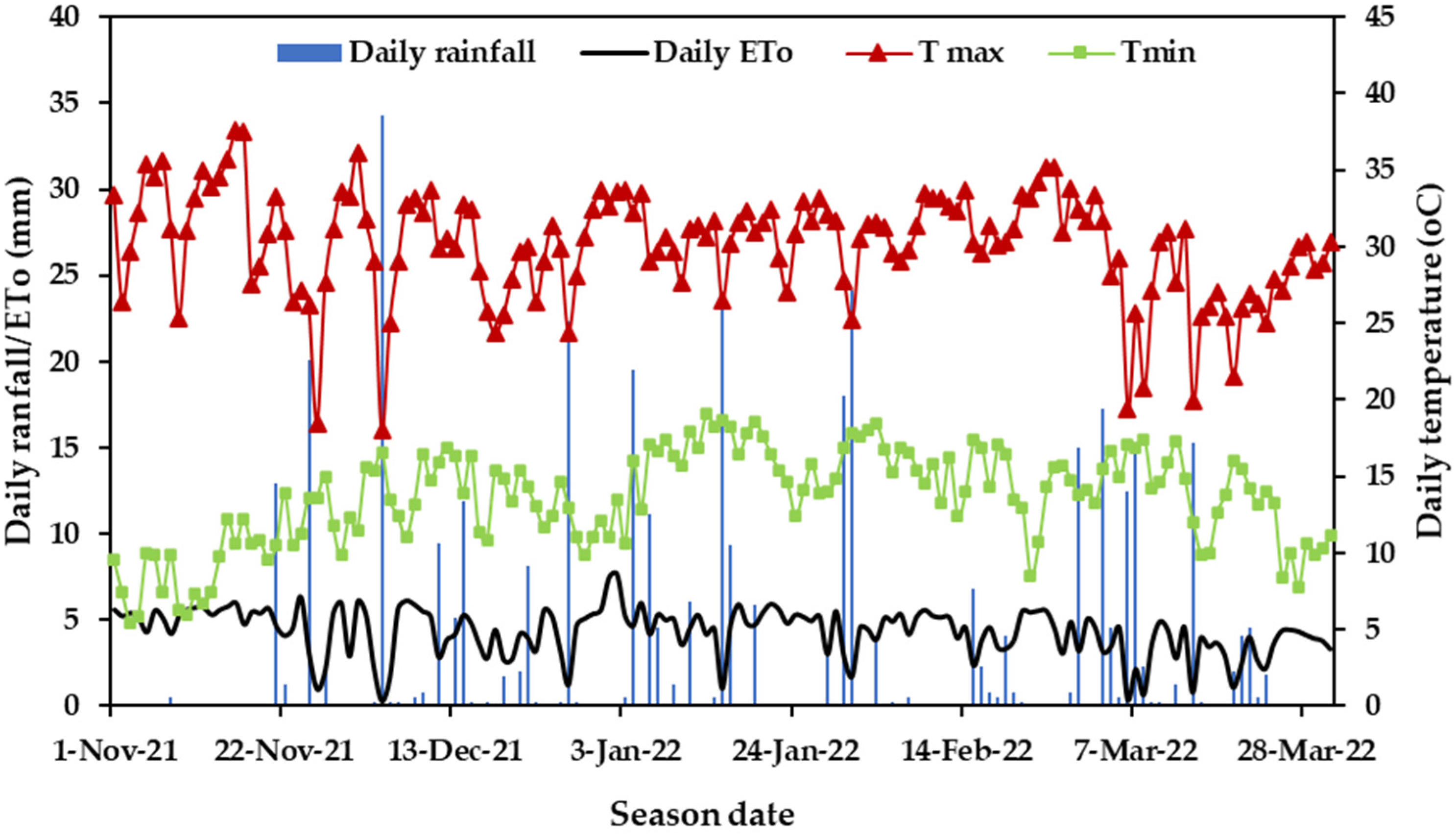
3.1. Weather Conditions during the Growing Season

The daily weather data observed in the WFS during the potato growing season are shown in Figure 2. Daily rainfall was evenly distributed throughout the growing months, and at least two rainfall events of ≥15 mm were received each month. The mean daily maximum temperature (Tmax) oscillated around 30 °C, while the mean daily minimum temperature (Tmin) was approximately 15 °C for most days. The observed mean daily ETo for most days during the season was 5 mm day⁻¹. Lower values of daily Tmax, Tmin, and ETo were recorded on days when substantial rainfall occurred (Figure 2).

3.2. Growing Season Length, Rainfall, Irrigation, Drainage and Seasonal Reference Evapotranspiration

Table 4. Growing season length, rainfall, effective irrigation, drainage, and seasonal reference evapotranspiration (ETo) for Fields 2–6.

Field No.	Growing Season Length (days)	Rainfall (mm)	Effective Irrigation (mm)	Drainage (mm)	Seasonal ETo (mm)
2	117	298	399	89	608
3	125	374	391	103	639
4	112	253	217	63	554
5	111	291	182	12	560
6	112	344	165	7	550
Average	115	312	271	55	582

presents the length of the growing season, accumulated rainfall, effective irrigation, drainage, and seasonal reference evapotranspiration for Fields 2–6. These variables were not measured in Field 1. The length of the growing season ranged from 107 to 125 days with a mean of 115 days. The mean accumulated rainfall received was 312 mm, representing 53% of the total mean water input. The effective irrigation applied varied greatly across the fields and ranged between 165 and 399 mm (mean 271 mm). The observed drainage varied substantially between fields and ranged between 7 and 103 mm. Fields that received the highest amount of total water through rainfall and irrigation also recorded the highest drainage. Fields 2 and 3 recorded the highest drainage of 89 and 103 mm, respectively. The drainage for Fields 2, 3 and 4 equaled 13% of the total water input. The accumulated ETo ranged between 548 and 639 mm, with a mean value of 582 mm, showing little variation in the atmospheric evaporative demand across the crop season between the fields (Table 4).

A comparison between the effective actual irrigation and simulated irrigation requirement by the LINTUL-Potato model is presented in Figure 3. Fields 2 and 3 received 76 and 49 mm more actual irrigation than the simulated irrigation requirement. This suggests that Fields 2 and 3 received more irrigation water than what was required. In contrast, Fields 4–6 received substantially lower actual irrigation amounts than the modelled requirements. The difference between the actual irrigation and the modelled irrigation requirements for Fields 4–6 ranged from −84 to −125 mm.

3.3. Crop Canopy Growth and Development

The changes in crop canopy growth and development variables as well as observed NDVI over the growing season for Fields 1–6 combined are presented in Figure 4. All crop canopy growth variables showed a similar trend from emergence to maximum canopy growth, which was attained at about 60 DAP. The minimum NDVI for bare soil was 0.13, while the maximum NDVI of approximately 0.84 was attained at about 50 DAP (Figure 4a). The maximum NDVI remained constant between 50 and 100 DAP and thereafter started declining, indicating the onset of crop senescence. Maximum FIPAR of 0.95 was attained at 60 DAP (Figure 4b), mean maximum LAI of about 3.8 m² m⁻² was attained at 65 DAP (Figure 4c) and maximum GCC of approximately 95% was attained at about 65 DAP (Figure 4d). The canopy growth curves for NDVI, FIPAR, and GCC showed that the approximate length of the crop development stage was about 40 days (from 20 to 60 DAP), the length of the mid-season stage was about 40 days (from 60 to 100 DAP), and the length of the late-season stage was between 15 and 20 days, depending on when vines were killed off.

3.4. Relationship between Leaf Area Index and NDVI

The empirical relationship between LAI and NDVI is presented in Figure 5a. The nonlinear relationship between LAI and NDVI followed an exponential trend, where NDVI saturation occurred at an LAI of about 3.5 m² m⁻². The observed data from Fields 1 and 2 were fitted with an exponential function similar to Equation (13), producing a line of best fit with a coefficient of determination (R²) of 0.97, and a coefficient $M$ of 0.99 (Figure 5a). Therefore, the ratio of the coefficients N and M ($\frac{N}{M})$ in Equation (16) was 0.61 (0.60/0.99). The fitted relationship resulted in a maximum NDVI (${VI}_{max}$) of 0.85 and a minimum NDVI of 0.13 corresponding to bare soil (${VI}_{min}$). The maximum and minimum NDVI values of the fitted empirical relationship are comparable with the observed values during the season. The generated NDVI-LAI relationship was tested against an independent dataset from Fields 3–6, and the results showed a relatively good agreement between the observed NDVI and the fitted (modelled) NDVI values, with R² = 0.92 and RMSE = 0.069 (Figure 5b).

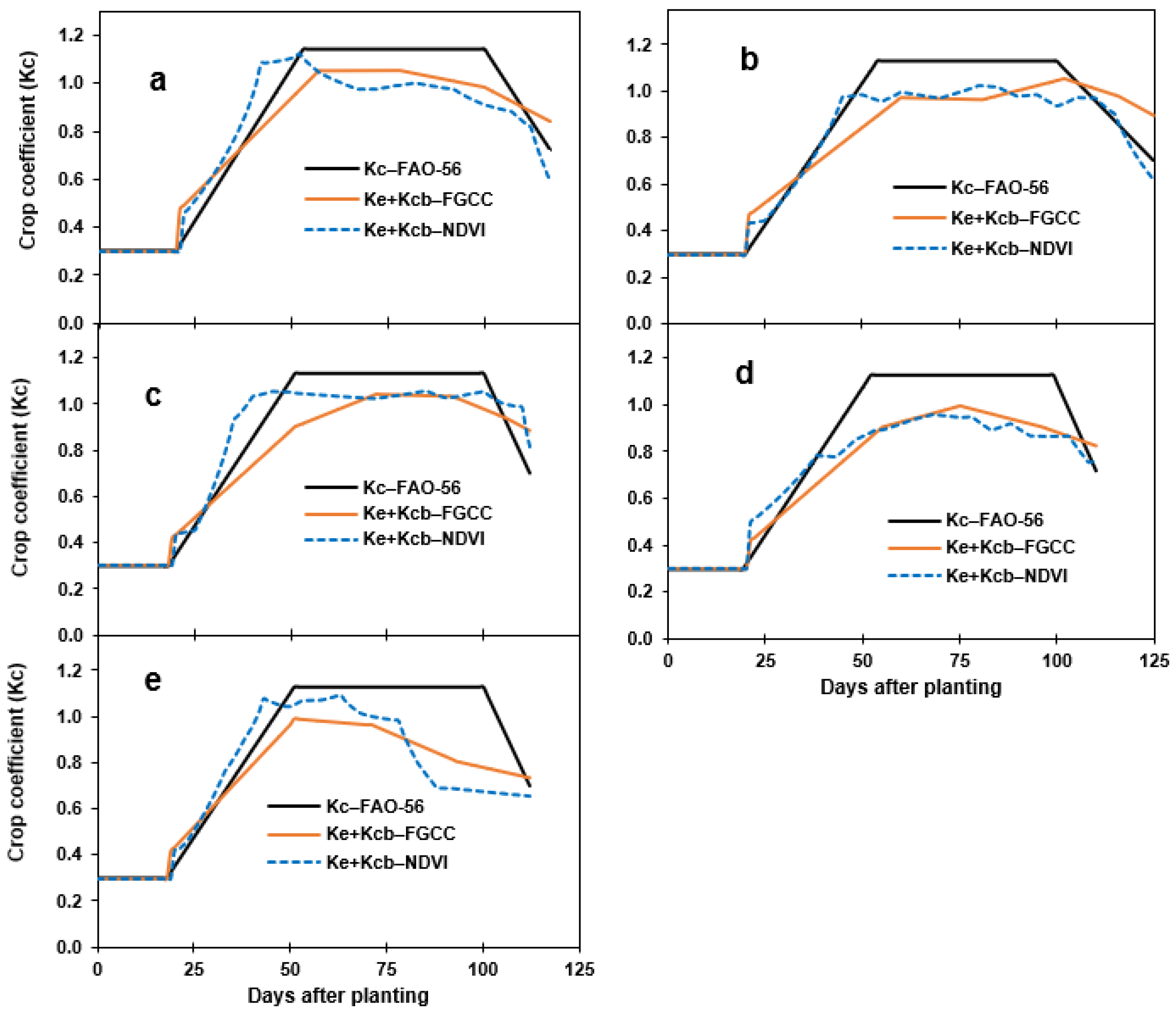
3.5. Comparison of Crop Coefficients for the Different Approaches

Figure 6 shows the Kc curves using the different approaches for Fields 2–6. The Kc during the initial stage was maintained at 0.30 for all approaches. The Kc curves based on the FAO-56 approach were similar for Fields 2–6. The Kc in this approach increased linearly from 0.30 to a maximum value of 1.13 during the crop development stage, remained constant during the mid-season stage, and thereafter declined to a final value of 0.70 during the late-season growth stage (Figure 6). The mean Kc values in this approach for the initial, development, mid-season, and late-season stages were 0.30, 0.71, 1.13, and 0.91, respectively (

Table 5. Comparison of the mean crop coefficients (Kc) for FAO-56, Kcb-FGCC and Kcb-NDVI approaches for the initial, development (Dev), mid-season (Mid) and late-season (Late) growth stages for Fields 2–6.

Field No.	Kc = FAO-56				Kc = Kcb-FGCC				Kc = Kcb-NDVI
	Initial	Dev	Mid	Late	Initial	Dev	Mid	Late	Initial	Dev	Mid	Late
2	0.30	0.72	1.14	0.92	0.30	0.72	1.03	0.91	0.30	0.84	0.99	0.82
3	0.30	0.71	1.13	0.91	0.30	0.68	0.98	0.99	0.30	0.71	0.99	0.86
4	0.30	0.71	1.13	0.90	0.30	0.65	1.01	0.93	0.30	0.79	1.03	0.98
5	0.30	0.71	1.13	0.91	0.30	0.63	0.94	0.86	0.30	0.71	0.92	0.82
6	0.30	0.70	1.13	0.90	0.30	0.69	0.91	0.76	0.30	0.79	0.90	0.66
Mean	0.30	0.71	1.13	0.91	0.30	0.67	0.97	0.89	0.30	0.77	0.97	0.83

).

The Kc curves based on the Kcb-FGCC approach varied across the fields, reflecting differences in GCC between fields (Figure 6). The curves demonstrated a gradual increase in Kc during the development stage with a peak Kc value of about 1.0 between 55 and 60 DAP. The Kc remained relatively stable until the crop was killed off. The observed change in Kc using the Kcb-FGCC approach was slightly lower than the change in Kc for the FAO-56 approach for all the crop stages (Figure 6). In Field 6, the Kc profile developed at a lower rate compared to the other fields, reflecting the poor canopy cover observed in this field (Figure 6e). The mean Kc values in the Kcb-FGCC approach for the initial, development, mid-season, and late-season growth stages were 0.30, 0.67, 0.97, and 0.89, respectively (Table 5).

The Kc curves based on the Kcb-NDVI approach followed a similar trend to that observed for the seasonal NDVI curves (Figure 4a). The increase in Kc during the development stage was slightly higher than that observed in both the FAO-56 and Kcb-FGCC approaches, which reflected a fast increase in NDVI from emergence to 100% canopy cover. The Kcb-NDVI approach provided a slightly lower Kc during the mid-season growth stage than the FAO-56 approach. On average, the Kc for the Kcb-NDVI approach was 0.16 lower than the Kc values for the FAO-56 approach (Table 5). Field 6 showed a relatively low NDVI following poor canopy growth during the season. Therefore, it had the lowest Kc in the Kcb-NDVI approach (Figure 6e). The mean Kc values for the Kcb-NDVI approach for the initial, development, mid-season, and late-season growth stages were 0.30, 0.77, 0.97, and 0.83, respectively (Table 5).

3.6. Evapotranspiration Estimate by the LINTUL Model

A comparison of crop ET derived from the three methods with ET simulated by the LINTUL-Potato model is illustrated in Figure 7. ET estimated by the LINTUL-Potato model ranged between 415–505 mm, with a mean of 449 mm. Crop ET for FAO-56 approach ranged between 466–532 mm, with a mean of 489 mm. The ET for the Kcb-FGCC approach ranged between 401–494 mm (mean of 442 mm), while ET for the Kcb-NDVI approach ranged between 410–492 mm (mean of 450 mm) (Figure 7 and

Table 6. Summary of root mean square error (RMSE) and mean absolute error (MAE) obtained by comparing the ET estimated by the LINTUL-Potato model with the ET based on the FAO-56 approach (ET-FAO-56), the Kcb-FGCC approach (ET-Kcb-FGCC) and the Kcb-NDVI approach (ET-Kcb-NDVI).

Field No.	ET-FAO-56 (mm day−1)		ET-Kcb-FGCC (mm day−1)		ET-Kcb-NDVI (mm day−1)
	RMSE	MAE	RMSE	MAE	RMSE	MAE
2	0.91	0.77	0.76	0.52	0.75	0.50
3	0.89	0.75	0.81	0.53	0.79	0.51
4	0.77	0.63	0.73	0.51	0.60	0.36
5	0.82	0.69	0.86	0.66	0.81	0.65
6	0.74	0.61	0.79	0.63	0.92	0.68
All	0.83	0.69	0.79	0.57	0.78	0.54

). ET derived by the FAO-56 approach were 5–12% higher than the modelled ET for all fields. ET derived by the Kcb-FGCC and Kcb-NDVI approaches were 2–6% lower than the modelled ET for Fields 3, 5 and 6 (Figure 7). Although actual ET was not measured directly in the fields, the ET values calculated by the LINTUL-Potato model were assumed to be reasonably accurate, as the model was parameterized for each field, and compared well with measurements in previous local studies [3,35].

A comparison between simulated ET and ET derived by the FAO-56 approach gave an overall RMSE of 0.83 and a MAE of 0.69 mm day⁻¹ (Table 6). The variation between simulated and Kcb-FGCC approach ET resulted in an overall RMSE of 0.79 and an MAE of 0.57 mm day⁻¹. The comparison between simulated ET and ET derived from the Kcb-NDVI approach showed the lowest overall RMSE of 0.78 mm day⁻¹ and an MAE of 0.54 mm day⁻¹ (Table 6).

3.7. Yield and Water Use Efficiency

Relatively high fresh tuber yield was obtained for Fields 2–6 with values between 69–114 t ha⁻¹ and a mean of 95.7 t ha⁻¹ (

Table 7. Tuber yield and water use efficiency (WUE) based on rainfall and irrigation (WUE_R+I) and WUE based on evapotranspiration (ET) estimated for; FAO-56 approach (WUE_{ET_FAO}), Kcb-FGCC approach (WUE_{ET_FGCC}), Kcb-NDVI approach (WUE_{ET_NDVI}) and WUE based on ET simulated by LINTUL model (WUE_{ET_LINTUL}).

Field No.	Fresh Tuber Yield (t ha−1)	WUER+I (kg ha−1 mm−1)	WUEET_FAO (kg ha−1 mm−1)	WUEET_FGCC (kg ha−1 mm−1)	WUEET_NDVI (kg ha−1 mm−1)	WUEET_LINTUL (kg ha−1 mm−1)
2	91	130.3	178.0	188.0	188.4	192.4
3	110	144.3	207.5	223.5	224.4	218.6
4	114	241.9	241.4	265.0	246.1	267.5
5	94	199.2	202.1	233.7	232.0	220.6
6	69	136.3	148.9	173.1	169.3	167.2
Mean	95.7	170.4	195.6	216.7	212.0	213.3

). Field 4 achieved the highest yield of 114 t ha⁻¹ and Field 6 the lowest (69 t ha⁻¹). The high yield observed in Field 4 resulted in the highest WUE_R+I (Table 7). Despite a substantially lower yield, Field 6 had a WUE_R+I comparable to Fields 2 and 3, suggesting that the high total water input applied in Fields 2 and 3 did not necessarily lead to more tuber yield (Figure 2). The low WUE_R+I for Field 6 was due to lower tuber yield observed, even though relatively low amounts of water were applied to this field. The WUE_ET was calculated for each ET estimation approach as well for the LINTUL-Potato model (Table 7). The FAO-56 approach provided the lowest WUE_ET due to the highest ET derived, and ranged between 148.9–241.4 kg ha⁻¹ mm⁻¹ (mean of 195.6 kg ha⁻¹ mm⁻¹). The WUE_ET for the Kcb-FGCC and Kcb-NDVI approaches were comparable to the WUE_ET from the LINTUL-Potato model. The mean WUE_ET based on ET estimated from the Kcb-FGCC, Kcb-NDVI and LINTUL-Potato model were 216.7, 212.0 and 213.3 kg ha⁻¹ mm⁻¹, respectively (Table 7).

4. Discussion

Substantial rainfall was received during the potato season, contributing to more than half the total water input in all fields. Variation in water input across fields reflected differences in irrigation applied. Irrigation applied in Fields 2 and 3 exceeded the simulated irrigation requirements substantially, suggesting that these fields were over-irrigated. Fields 3, 4 and 5 applied less irrigation water amounts and still obtained good yields. This indicates that smart water application by reducing both the number of irrigation events and irrigation depth is feasible without a yield penalty, especially during seasons with above normal rainfall.

As expected, fields where the total water inputs exceeded seasonal ETo recorded the highest drainage. It is well documented that drainage in sandy soils increases with greater total water input [36,37]. The risk of drainage in sandy soils with a lower water holding capacity is high after a major rain event. As rainfall forecasts are inherently uncertain, growers usually leave no room for uncertain rainfall because the risk of crop water stress is high when potatoes are grown on sandy soils in a semi-arid region. Therefore, under these conditions, drainage can be minimized by precise irrigation using accurate estimations of crop water requirements.

The close similarity in the temporal trends observed for NDVI, GCC, FIPAR, and LAI suggests that potato phenology can be remotely monitored using NDVI. As the season progresses, the greenness of the crop increases, providing distinct and detectable spectral signatures which change with growth stages [38]. Remotely sensed phenology information therefore offers a more dynamic approach to the development of Kc than the FAO-56 approach. Moreover, generating Kc curves from FGCC and NDVI temporal trends does not require knowledge of the length of the growth stages as opposed to the FAO-56 Kc curves [39].

Remote sensing-based ET estimations require maximum values of NDVI, GCC, and LAI at full canopy cover [39]. Maximum NDVI of 0.85 at full canopy cover observed in the present study falls in the range of maximum NDVI of 0.8–0.9 reported for potatoes in previous studies [40,41,42]. The observed peak value of GCC percentage was 95%, which was slightly higher than the mean value of 88% reported by Pereira et al. [43]. The mean maximum LAI at full canopy cover observed for all fields was about 3.5 m² m⁻² and was in line with LAI values reported for potato at full canopy cover [21,44], and other crops like soybean [24] and wheat [16].

In addition to the maximum and minimum values of VI, LAI, and GCC, the estimation of Kcb following the approach by Choudhury et al. [17] and Campos et al. [24] requires an analysis of the relationship between VI and LAI. In this study, the relationship between NDVI and LAI showed that NDVI saturates at LAI of about 3.5 m² m⁻², which agrees with the findings from previous studies [16,24]. Although NDVI saturates at LAI >3 m² m⁻², it has been reported to be a better predictor of Kcb than SAVI [45,46]. This is because NDVI reaches its maximum value at approximately the same time as Kcb, whereas SAVI continues to increase with LAI,0020resulting in an underestimation of the maximum Kcb [43]. The observed value of the coefficient $M$ of 0.99 falls in the range of 0.80–1.30 proposed by Choudhury et al. [17]. Campos et al. [24] observed a lower $M$ value of 0.62 for both maize and soybean from the NDVI-LAI relationship.

The Kc values based on the FGCC and NDVI compared relatively well with Kc values based on the FAO-56 approach, as well as with values reported in other studies (

Table 8. Comparison of crop coefficients (Kc) of potato varieties grown in different regions for the initial, development, mid-season and late-season growth stages.

Study	Study Area	Climate	Methodology	Variety	Initial	Development	Mid- Season	Late- Season
This study [10]	South Africa	Semi-arid	FAO-56	Mondial	0.30	0.71	1.13	0.91
This study	South Africa	Semi-arid	Kcb-FGCC	Mondial	0.30	0.67	0.97	0.89
This study	South Africa	Semi-arid	Kcb-NDVI	Mondial	0.30	0.77	0.97	0.83
[49]	South Africa	Semi-arid	Pan evap.	Up-to-Date	0.45	0.65	0.83	0.60
[47]	South Africa	Semi-arid	ECV	Mondial	-	1.00	1.15	0.87
[47]	South Africa	Semi-arid	ECV	Mondial	-	0.45	0.86	-
[50]	India	Semi-arid	SWB	Kufri Pukraj	-	0.55	1.11	1.01
[51]	USA	Arid	SWB	Russet varieties	0.40	-	0.95	0.57
[52]	USA	Arid	SWB	Russet Burbank	0.30	0.69	0.93	0.50

USA is United States of America, Pan evap. is pan evaporation, ECV is eddy covariance, SWB is soil water balance.

). However, Kc based on the FAO-56 approach was on average 0.16 (14.2%) higher than the Kc values from the Kcb-FGCC and Kcb-NDVI approaches during the mid-season growth stage. Likewise, the Kc value of 1.15 observed during the tuber initiation (mid-season) stage in the Limpopo Province of South Africa [47] was higher than the values observed for the Kcb-FGCC and Kcb-NDVI approaches in the present study (Table 8). Johnson and Trout [48] found that the Kcb values based on fractional canopy cover for different vegetable crops (broccoli, garlic, lettuce and bell pepper) were 6–10% lower than the Kcb provided by the FAO-56 paper for the mid-season growth stage.

The Kc or Kcb values based on FGCC and NDVI are influenced by crop canopy growth and ground coverage, which depend on various factors, such as nutrient and water availability, the incidence of pests and diseases, and extreme weather conditions (frost and hail). These factors may result in reduced canopy coverage and affect crop reflectance properties, leading to errors in the observed GCC and NDVI values [8]. Moreover, prolonged periods of overcast sky hinder satellite imagery acquisition, which increases the uncertainty in the Kcb-NDVI profiles generated using interpolated NDVI over longer intervals [11]. During the current season, NDVI was not available on at least four dates for each field due to overcast conditions, and most of these days coincided with the mid-season stage. Johnson and Trout [48] also mentioned that Kcb based on fractional cover is more sensitive to measurement errors during the linear phase (mid-season stage) of the Kcb curves.

Compared to ET simulated by the LINTUL-Potato model, the FAO-56, Kcb-FGCC and Kcb-NDVI approaches estimated ET with RMSE between 0.78–0.83 mm day⁻¹, which falls in the range of widely accepted RMSE values by the ET community of between 0.2–0.9 mm day⁻¹ [53]. Crop ET generally depends on the water input levels, crop variety, soil type, and climatic conditions during the cropping season [30]. Therefore, direct ET comparisons with values obtained in previous studies may be inappropriate because climate and crop management are not the same. However, ET values for relatively similar climatic conditions can be compared. The seasonal ET values estimated by the three approaches in this study fall in the range of 338–579 mm reported for potato in comparable semi-arid regions of South Africa [47,54]. Ierna and Mauromicale [55] reported a potato seasonal ET of 411 and 448 mm for two consecutive years in a semi-arid region of southern Italy. Similarly, Kiziloglu et al. [56] reported potato ET values of 415 and 475 mm over two consecutive seasons in a semi-arid region of Turkey. Using the soil water balance approach, Djaman et al. [30] obtained potato seasonal ET values between 534–681 mm over two seasons in a semi-arid climate. In the same study, the FAO-56 single crop coefficient approach showed ET values between 796–833 mm, whereas satellite modelled ET over the same period of study ranged between 437–625 mm.

To the best of our knowledge, few studies have assessed the ET of crops using FGCC and a modified analytical approach to the Kcb-NDVI relationship. Seasonal ET observed for the Kcb-FGCC and Kcb-NDVI approaches compared relatively well with simulated ET by the LINTUL-Potato model, with RMSE of 0.79 and 0.78 mm day⁻¹. These RMSE values are similar to those reported by other authors for different crops, including wheat, RMSE = 0.40–1.47 mm day⁻¹ [19,33,57], maize, RMSE = 0.56–1.06 mm day⁻¹ [24], cotton, RMSE = 0.6–1.12 mm day⁻¹ [12,58,59] and soybean, RMSE = 0.77–1.01 mm day⁻¹ [24]. Therefore, the results of this study indicate that Kcb-FGCC and Kcb-NDVI approaches offer alternative ways to estimate potato daily ET using real-time canopy information.

WUE is a function of crop genetics, management practices, irrigation levels and climatic conditions [60]. The high tuber yields observed reflected good crop management, as well as favorable environmental growing conditions. In all fields, potato was grown primarily for seed production, therefore, the growers applied intense management. The two fields that received substantially higher total water input (Fields 2 and 3), also had high yields, which resulted in a good WUE. The WUE_R+I and WUE_ET observed for all fields were similar to values reported by Machakaire et al. [47] (163–189 kg mm⁻¹) for potato produced under comparable conditions. Similarly, a WUE_R+I above 116 kg mm⁻¹ has been reported for other modern potato varieties elsewhere [61,62].

5. Conclusions

• A close association between NDVI development over the season and the development of GCC and FIPAR suggest that NDVI can be successfully used to remotely monitor potato phenology during the season.
• Canopy variables (GCC, FIPAR and LAI) indicate that effective canopy cover was attained at GCC of 95%, FIPAR of 0.9, LAI of 3.5 m² m⁻² and NDVI of 0.85. The NDVI-LAI relationship was observed to saturate at LAI of about 3.5 m² m⁻².
• In comparison with the FAO-56 approach, Kc values based on FGCC and NDVI were slightly lower during the mid-season season growth stage. However, the Kc profiles based on FGCC and NDVI represented actual crop development and were therefore expected to be more accurate than the FAO-56 approach.
• Seasonal ET based on the Kcb-FGCC and Kcb-NDVI approaches compared well with ET simulated by the LINTUL-Potato model. This suggested that Kcb-FGCC and Kcb-NDVI approaches offer alternative ways of estimating crop ET using readily available ETo and NDVI or canopy variable information. These results reinforce the utility of the modified analytical approach proposed by Choudhury et al. [17] and modified by Campos et al. [24] for potato ET estimation to facilitate irrigation management.

References

1. Stevens, J.; Sanewe, A.; Steyn, J.M.; Annandale, J.G.; Stirzaker, R.J. Improving On-Farm Irrigation Water and Solute Management Using Simple Tools and Adaptive Learning; Report No. TT821/20; Water Research Commission: Pretoria, South Africa, 2020; 188p. [Google Scholar]
2. Basson, M.S. Water development in South Africa. In Proceedings of the Water in the Green Economy in Practice: Towards Rio+20, Zaragoza, Spain, 3–5 October 2011. [Google Scholar]
3. Franke, A.C.; Steyn, J.M.; Ranger, K.S.; Haverkort, A.J. Developing environmental principles, criteria, indicators and norms for potato production in South Africa through field surveys and modelling. Agric. Syst. 2011, 104, 297–306. [Google Scholar] [CrossRef]
4. Steyn, J.M.; Franke, A.C.; van der Waals, J.E.; Haverkort, A.J. Resource use efficiencies as indicators of ecological sustainability in potato production: A South African case study. Field Crops Res. 2016, 199, 136–149. [Google Scholar] [CrossRef]
5. Machakaire, A.T.B.; Steyn, J.M.; Caldiz, D.O.; Haverkort, A.J. Forecasting yield and tuber size of processing potatoes in South Africa using the LINTUL-Potato-DSS Model. Potato Res. 2016, 59, 195–206. [Google Scholar] [CrossRef]
6. Charlesworth, P. Soil Water Monitoring. In Soil Water and Ground Water Sampling; CSIRO Land and Water: Canberra, Australia, 2000; 100p. [Google Scholar]
7. Annandale, J.G.; Stirzaker, R.J.; Singels, A.; van der Laan, M.; Laker, M.C. Irrigation scheduling research: South African experiences and future prospects. Water SA 2011, 37, 751–764. [Google Scholar] [CrossRef]
8. Allen, R.G.; Pereira, L.S.; Howell, T.A.; Jensen, M.E. Evapotranspiration information reporting: I. Factors governing measurement accuracy. Agric. Water Manag. 2011, 98, 899–920. [Google Scholar] [CrossRef]
9. De Jager, J.; Van Zyl, W. Atmospheric evaporative demand and evaporation coefficient concepts. Water SA 1989, 15, 103–110. [Google Scholar]
10. Allen, R.G.; Pereira, L.S.; Raes, D.; Smith, M. Crop Evapotranspiration (Guidelines for Computing Crop Water Requirements. FAO Irrigation and Drainage Paper No.56; FAO: Rome, Italy, 1998; Volume 56, pp. 1–333. [Google Scholar]
11. Pôças, I.; Calera, A.; Campos, I.; Cunha, M. Remote sensing for estimating and mapping single and basal crop coefficients: A review on spectral vegetation indices approaches. Agric. Water Manag. 2020, 233, 106081. [Google Scholar] [CrossRef]
12. Mateos, L.; González-Dugo, M.P.; Testi, L.; Villalobos, F.J. Monitoring evapotranspiration of irrigated crops using crop coefficients derived from time series of satellite images. I. Method validation. Agric. Water Manag. 2013, 125, 81–91. [Google Scholar] [CrossRef]
13. Neale, C.M.U.; Jayanthi, H.; Wright, J.L. Irrigation water management using high resolution airborne remote sensing. Irrig. Drain. Syst. 2005, 19, 321–336. [Google Scholar] [CrossRef]
14. Bausch, W.C. Soil background effects on reflectance-based crop coefficients for corn. Remote Sens. Environ. 1993, 46, 213–222. [Google Scholar] [CrossRef]
15. González-Dugo, M.P.; Mateos, L. Spectral vegetation indices for benchmarking water productivity of irrigated cotton and sugarbeet crops. Agric. Water Manag. 2008, 95, 48–58. [Google Scholar] [CrossRef]
16. Duchemin, B.; Hadria, R.; Erraki, S.; Boulet, G.; Maisongrande, P.; Chehbouni, A.; Escadafal, R.; Ezzahar, J.; Hoedjes, J.C.B.; Kharrou, M.H.; et al. Monitoring wheat phenology and irrigation in Central Morocco: On the use of relationships between evapotranspiration, crops coefficients, leaf area index and remotely-sensed vegetation indices. Agric. Water Manag. 2006, 79, 1–27. [Google Scholar] [CrossRef]
17. Choudhury, B.J.; Ahmed, N.U.; Idso, S.B.; Reginato, R.J.; Daughtry, C.S.T. Relations between evaporation coefficients and vegetation indices studied by model simulations. Remote Sens. Environ. 1994, 50, 1–17. [Google Scholar] [CrossRef]
18. Glenn, E.P.; Neale, C.M.U.; Hunsaker, D.J.; Nagler, P.L. Vegetation index-based crop coefficients to estimate evapotranspiration by remote sensing in agricultural and natural ecosystems. Hydrol. Process. 2011, 25, 4050–4062. [Google Scholar] [CrossRef]
19. Hunsaker, D.J.; Pinter, P.J.; Kimball, B.A. Wheat basal crop coefficients determined by normalized difference vegetation index. Irrig. Sci. 2005, 24, 1–14. [Google Scholar] [CrossRef]
20. Barker, J.B.; Heeren, D.M.; Neale, C.M.U.; Rudnick, D.R. Evaluation of variable rate irrigation using a remote-sensing-based model. Agric. Water Manag. 2018, 203, 63–74. [Google Scholar] [CrossRef]
21. Jayanthi, H.; Neale, C.M.U.; Wright, J.L. Development and validation of canopy reflectance-based crop coefficient for potato. Agric. Water Manag. 2007, 88, 235–246. [Google Scholar] [CrossRef]
22. Er-Raki, S.; Rodriguez, J.C.; Garatuza-Payan, J.; Watts, C.J.; Chehbouni, A. Determination of crop evapotranspiration of table grapes in a semi-arid region of Northwest Mexico using multi-spectral vegetation index. Agric. Water Manag. 2013, 122, 12–19. [Google Scholar] [CrossRef]
23. Jin, X.; Yang, G.; Xue, X.; Xu, X.; Li, Z.; Feng, H. Validation of two Huanjing-1A/B satellite-based FAO-56 models for estimating winter wheat crop evapotranspiration during mid-season. Agric. Water Manag. 2017, 189, 27–38. [Google Scholar] [CrossRef]
24. Campos, I.; Neale, C.M.U.; Suyker, A.E.; Arkebauer, T.J.; Gonçalves, I.Z. Reflectance-based crop coefficients REDUX: For operational evapotranspiration estimates in the age of high producing hybrid varieties. Agric. Water Manag. 2017, 187, 140–153. [Google Scholar] [CrossRef]
25. Moeletsi, M.E.; Walker, S. Rainy season characteristics of the Free State Province of South Africa with reference to rain-fed maize production. Water SA 2012, 38, 775–782. [Google Scholar] [CrossRef]
26. Kruger, A.C.; Mbatha, S. Regional Weather and Climate of South Africa: Gauteng; South African Weather Service: Pretoria, South Africa, 2021.
27. Kooman, P.L.; Haverkort, A.J. Modelling development and growth of the potato crop influenced by temperature and daylength: LINTUL-POTATO. In Potato Ecology and Modelling of Crops under Conditions Limiting Growth, 1st ed.; Haverkort, A.J., MacKerron, D.K.L., Eds.; Kluwer Academic Publishers: Dordrecht, The Netherlands, 1995; pp. 41–60. [Google Scholar]
28. Alva, A.; Fan, M.; Qing, C.; Rosen, C.; Ren, H. Improving nutrient-use efficiency in chinese potato production: Experiences from the United States. J. Crop Improv. 2011, 25, 46–85. [Google Scholar] [CrossRef]
29. Iwama, K. Physiology of the potato: New insights into root system and repercussions for crop management. Potato Res. 2008, 51, 333–353. [Google Scholar] [CrossRef]
30. Djaman, K.; Koudahe, K.; Saibou, A.; Darapuneni, M.; Higgins, C.; Irmak, S. Soil water dynamics, effective rooting zone, and evapotranspiration of sprinkler irrigated potato in a sandy loam soil. Agronomy 2022, 12, 864. [Google Scholar] [CrossRef]
31. Patrignani, A.; Ochsner, T.E. Canopeo: A powerful new tool for measuring fractional green canopy cover. Agron. J. 2015, 107, 2312–2320. [Google Scholar] [CrossRef]
32. Haverkort, A.J. Potato Handbook: Crop of the Future; Aardappelwereld BV: The Hague, The Netherlands, 2018; p. 592. [Google Scholar]
33. Er-Raki, S.; Chehbouni, A.; Duchemin, B. Combining satellite remote sensing data with the FAO-56 dual approach for water use mapping in irrigated wheat fields of a semi-arid region. Remote Sens. 2010, 2, 375–387. [Google Scholar] [CrossRef]
34. Franke, A.C.; Haverkort, A.J.; Steyn, J.M. Climate change and potato production in contrasting South African agro-ecosystems 2. Assessing risks and opportunities of adaptation strategies. Potato Res. 2013, 56, 51–66. [Google Scholar] [CrossRef]
35. Haverkort, A.J.; Franke, A.C.; Steyn, J.M.; Pronk, A.; Caldiz, D.; Kooman, P. A robust potato model: LINTUL-POTATO-DSS. Potato Res. 2015, 58, 313–327. [Google Scholar] [CrossRef]
36. Prasad, R.; Hochmuth, G.J.; Boote, K.J. Estimation of nitrogen pools in irrigated potato production on sandy soil using the model SUBSTOR. PLoS ONE 2015, 1, e0117891. [Google Scholar] [CrossRef]
37. Clément, C.C.; Cambouris, A.N.; Ziadi, N.; Zebarth, B.J.; Karam, A. Potato yield response and seasonal nitrate leaching as influenced by nitrogen management. Agronomy 2021, 11, 2055. [Google Scholar] [CrossRef]
38. Gobin, A.; Sallah, A.H.M.; Curnel, Y.; Delvoye, C.; Weiss, M.; Wellens, J.; Piccard, I.; Planchon, V.; Tychon, B.; Goffart, J.P.; et al. Crop phenology modelling using proximal and satellite sensor data. Remote Sens. 2023, 15, 2090–2109. [Google Scholar] [CrossRef]
39. Irmak, S.; Odhiambo, L.O.; Specht, J.E.; Djaman, K. Hourly and daily single and basal evapotranspiration crop coefficients as a function of growing degree days, days after emergence, leaf area index, fractional green canopy cover, and plant phenology for soybean. Trans. ASABE 2013, 56, 1785–1803. [Google Scholar]
40. Bala, S.K.; Islam, A.S. Correlation between potato yield and MODIS-derived vegetation indices. Int. J. Remote Sens. 2009, 30, 2491–2507. [Google Scholar] [CrossRef]
41. Johnson, D.M. A comprehensive assessment of the correlations between field crop yields and commonly used MODIS products. Int. J. Appl. Earth Obs. Geoinf. 2016, 52, 65–81. [Google Scholar] [CrossRef]
42. Newton, I.H.; Tariqul Islam, A.F.M.; Saiful Islam, A.K.M.; Tarekul Islam, G.M.; Tahsin, A.; Razzaque, S. Yield prediction model for potato using Landsat time series images driven vegetation indices. Remote Sens. Earth Syst. Sci. 2018, 1, 29–38. [Google Scholar] [CrossRef]
43. Pereira, L.S.; Paredes, P.; López-Urrea, R.; Hunsaker, D.J.; Mota, M.; Mohammadi Shad, Z. Standard single and basal crop coefficients for vegetable crops, an update of FAO56 crop water requirements approach. Agric. Water Manag. 2021, 243, 106196. [Google Scholar] [CrossRef]
44. Wright, J.L. New evapotranspiration crop coefficients. J. Irrig. Drain. Div. 1982, 108, 57–74. [Google Scholar] [CrossRef]
45. Campos, I.; Neale, C.M.U.; Calera, A.; Balbontín, C.; González-Piqueras, J. Assessing satellite-based basal crop coefficients for irrigated grapes (Vitis vinifera L.). Agric. Water Manag. 2010, 98, 45–54. [Google Scholar] [CrossRef]
46. Pôças, I.; Paço, T.A.; Paredes, P.; Cunha, M.; Pereira, L.S. Estimation of actual crop coefficients using remotely sensed vegetation indices and soil water balance modelled data. Remote Sens. 2015, 7, 2373–2400. [Google Scholar] [CrossRef]
47. Machakaire, A.T.B.; Steyn, J.M.; Franke, A.C. Assessing evapotranspiration and crop coefficients of potato in a semi-arid climate using Eddy Covariance techniques. Agric. Water Manag. 2021, 255, 107029. [Google Scholar] [CrossRef]
48. Johnson, L.F.; Trout, T.J. Satellite NDVI assisted monitoring of vegetable crop evapotranspiration in california’s san Joaquin Valley. Remote Sens. 2012, 4, 439–455. [Google Scholar] [CrossRef]
49. Steyn, J.M.; Du Plessis, H.F. Soil, water and irrigation requirements of potatoes. In Guide to Potato Production in South Africa, 1st ed.; Denner, F.D., Venter, S., Niederwieser, J., Eds.; ARC-Roodeplaat, Vegetable and Ornamental Plants Institute: Pretoria, South Africa, 2012; pp. 123–134. [Google Scholar]
50. Kadam, S.A.; Gorantiwar, S.D.; Mandre, N.P.; Tale, D.P. Crop coefficient for potato crop evapotranspiration estimation by field water balance method in semi-arid region, Maharashtra, India. Potato Res. 2021, 64, 421–433. [Google Scholar] [CrossRef]
51. Gonzalez, T.F.; Pavek, M.J.; Holden, Z.J.; Garza, R. Evaluating potato evapotranspiration and crop coefficients in the Columbia Basin of Washington state. Agric. Water Manag. 2023, 286, 108371. [Google Scholar] [CrossRef]
52. Unites States Bureau of Reclaimation (USBR). Agrinet Crop Coefficients: Potatoes. 2016. Available online: https://www.usbr.gov/pn/agrimet/cropcurves/POTAcc.html (accessed on 28 July 2023).
53. Chakroun, H.; Zemni, N.; Benhamid, A.; Dellaly, V.; Slama, F.; Bouksila, F.; Berndtsson, R. Evapotranspiration in semi-arid climate:Remote sensing vs. soil water simulation. Sensors 2023, 23, 2823. [Google Scholar] [CrossRef]
54. Steyn, J.M.; Kagabo, D.M.; Annandale, J.G. Potato growth and yield responses to irrigation regimes in contrasting seasons of a subtropical region. In Proceedings of the 8th African Crop Science Society Conference, El-Minia, Egypt, 27–31 October 2007; pp. 1647–1651. [Google Scholar]
55. Ierna, A.; Mauromicale, G. Potato growth, yield and water productivity response to different irrigation and fertilization regimes. Agric. Water Manag. 2018, 201, 21–26. [Google Scholar] [CrossRef]
56. Kiziloglu, F.M.; Sahin, U.; Tune, T.; Diler, S. The effect of deficit irrigation on potato evapotranspiration and tuber yield under cool season and semi-arid climatic conditions. J. Agron. 2006, 5, 284–288. [Google Scholar]
57. French, A.N.; Hunsaker, D.J.; Sanchez, C.A.; Saber, M.; Gonzalez, J.R.; Anderson, R. Satellite-based NDVI crop coefficients and evapotranspiration with eddy covariance validation for multiple durum wheat fields in the US Southwest. Agric. Water Manag. 2020, 239, 106266. [Google Scholar] [CrossRef]
58. Hunsaker, D.J.; Barnes, E.M.; Clarke, T.R.; Fitzgerald, G.J.; Pinter, P.J. Cotton irrigation scheduling using remotely sensed and FAO-56 basal crop coefficients. Trans. Am. Soc. Agric. Eng. 2005, 48, 1395–1407. [Google Scholar] [CrossRef]
59. Hunsaker, D.J.; Pinter, P.J.; Barnes, E.M.; Kimball, B.A. Estimating cotton evapotranspiration crop coefficients with a multispectral vegetation index. Irrig. Sci. 2003, 22, 95–104. [Google Scholar] [CrossRef]
60. Onder, S.; Caliskan, M.E.; Onder, D.; Caliskan, S. Different irrigation methods and water stress effects on potato yield and yield components. Agric. Water Manag. 2005, 73, 73–86. [Google Scholar] [CrossRef]
61. Fandika, I.R.; Kemp, P.D.; Millner, J.P.; Horne, D.; Roskruge, N. Irrigation and nitrogen effects on tuber yield and water use efficiency of heritage and modern potato cultivars. Agric. Water Manag. 2016, 170, 148–157. [Google Scholar] [CrossRef]
62. Djaman, K.; Irmak, S.; Koudahe, K.; Allen, S. Irrigation management in potato (Solanum tuberosum L.) production: A Review. Sustainability 2021, 13, 1504. [Google Scholar] [CrossRef]
Figure 1. Canopeo® green canopy cover estimation as percentages.
Remotesensing 15 04579 g001
Figure 2. Daily rainfall, daily reference evapotranspiration (ETo), daily maximum (Tmax), and daily minimum (Tmin) temperatures observed during the potato growing season in the WFS region.
Remotesensing 15 04579 g002
Figure 3. Comparison of actual irrigation and irrigation water requirement simulated by the LINTUL-Potato model for Fields 2–6.
Remotesensing 15 04579 g003
Figure 4. Changes in crop development variables: (a) normalized vegetation index (NDVI); (b) fraction of intercepted photosynthetic active radiation (FIPAR); (c) leaf area index green; (d) canopy cover; over the growing season.
Remotesensing 15 04579 g004
Figure 5. Relationship between: (a) Leaf area index (LAI) and normalized difference vegetation index (NDVI) following the modified analytical approach to NDVI-LAI relationship by Choudhury et al. [17] and Campos et al. [24]; (b) Comparison between observed and fitted NDVI for the evaluation of the NDVI-LAI nonlinear equation.
Remotesensing 15 04579 g005
Figure 6. Comparison of the crop coefficient (Kc) curves from the FAO-56 approach (Kc-FAO-56), Ke+Kcb-FGCC approach and Ke+Kcb-NDVI approach for: (a) Field 2; (b) Field 3; (c) Field 4; (d) Field 5; (e) Field 6.
Remotesensing 15 04579 g006
Figure 7. Comparison of simulated evapotranspiration (ET) by LINTUL-Potato model with calculated ET using the FAO-56 approach (FAO-56), the Kcb-FGCC approach (Kcb-FGCC) and the Kcb-NDVI approach (Kcb-NDVI) for Fields 2–6.
Remotesensing 15 04579 g007