Estimating the Impacts of Ungauged Reservoirs Using Publicly Available Streamflow Simulations and Satellite Remote Sensing

Abstract

On the Korean Peninsula, the Imjin River is a transboundary river that flows from North Korea into South Korea. Therefore, human intervention activities in the upstream region can have a substantial impact on the downstream region of South Korea. In addition to climate impacts, there are increasing concerns regarding upstream man-made activities, particularly the operation of the Hwanggang dam located in the territory of North Korea. This study explored the feasibility of using the publicly available global hydrological model and satellite remote sensing imagery for monitoring reservoir dynamics and assessing their impacts on downstream hydrology. “Naturalized” streamflow simulation was obtained from the Group on Earth Observation (GEO) Global Water Sustainability (GEOGloWS) European Centre for Medium-Range Weather Forecasts (ECMWF) Streamflow Services (GESS) model. To correct the biases of the GESS-based streamflow simulations, we employed quantile mapping using the observed streamflow from a nearby location. This method significantly reduced volume and variability biases by up to 5 times on both daily and monthly scales. Nevertheless, its effectiveness in improving temporal correlation on a daily scale in small catchments remained constrained. For the reservoir storage changes in the Hwanggang dam, we combined multiple remote sensing imagery, particularly cloud-free optical images of Landsat-8, Sentinel-2, and snow-free Sentinel-1, with the area–elevation–volume (AEV) curves derived from the Shuttle Radar Topography Mission (SRTM) Digital Elevation Model (DEM). In assessing its hydrological impacts, the study found that overall impacts within the downstream catchment in Pilseung bridge of South Korea were generally less significant compared to the upstream Hwanggang catchment. However, there was a higher probability of experiencing water shortages during wet months due to the upstream dam’s operations. The study highlights the potential benefits of utilizing the publicly available hydrological model and satellite remote sensing imagery to supplement decision makers with important information for the effective management of the transboundary river basin in ungauged regions.

1. Introduction

Humans have constructed various water infrastructures, such as dams and reservoirs, to control the uneven spatial and temporal distribution of surface water resources. Over the past few decades, there has been a notable rise in the number of large dams, as reported by the International Commission on Large Dams (ICOLD) register. The most recent estimate as of April 2020 suggests that there are around 58,700 large dams worldwide [1]. Nonetheless, within international transboundary river basins, constructing large dams in upstream countries can potentially create hydro-political tensions as it significantly changes the water supply for downstream countries [2]. According to Gleick and Heberger [3], there were 109 recorded water-related conflicts from 2000 to 2012, with 24 of those being conflicts between different countries. For instance, it was believed that on 6 September 2009, Hwanggang dam’s unexpected release of 40 million cubic meters of water resulted in at least six deaths, and caused an estimated USD 500,000 in property damage on the downstream region of the Imjin River in South Korea [3,4]. Another example of deadly impacts from a dam failure occurred in southeast Laos in July 2018, and caused the destruction of thousands of hectares of agricultural land in Vietnam’s provinces of An Giang, Dong Thap, and Long An. The water levels in the Mekong River’s tributaries rose seven-to-ten centimeters daily, forcing thousands of individuals to evacuate and resulting in the loss of 27 lives in Laos [5]. Dam failures can be classified into two types: natural causes and human factors. Natural causes involve external factors like heavy rains, hurricanes and earthquakes, as well as internal factors such as aging materials and defects in the dam structure or foundations. Human factors include global climate warming, which contributes to increased extreme rainfall, glacial retreat, and the formation of glacial lakes that pose a dam break threat [6]. Dam failures typically result in significant loss of life, extensive destruction of properties, and severe environmental damage in the surrounding and downstream areas.

Therefore, it is essential to understand their operation patterns and hydrological impacts to design appropriate mitigation activities. However, access to available data in transboundary river basins is challenging, particularly in basins with intense geopolitical conflicts [7]. As societies in transboundary river basins are already interconnected on social and economic levels, concerns about water conflicts can lead to even higher political tensions, and such tensions are often the excuse for restricting data sharing. Meanwhile, even though international agreements exist in transboundary river basins that theoretically expect states to share data and information, they often have no binding enforcement mechanisms [8].

Satellite remote sensing has been increasingly utilized to supplement in situ measurements. One of its well-known applications in terrestrial water resources is obtaining surface water elevations from space through satellite radar altimeters, such as the Jason series and Envisat altimeters, which can provide highly accurate measurements (0.09–1.20 m), according to Okeowo et al. [9]. However, satellite radar altimetry is mostly effective for large bodies of water with minimal interference from surrounding terrain because of their large radar footprints, limiting their applications for smaller terrestrial water bodies. On the other hand, NASA’s Ice, Cloud, and Land Elevation Satellite (ICESAT) and ICESAT-2 laser altimeters can provide denser spatial coverage of the Earth’s water bodies, but with relatively low temporal resolution (~91 days). Additionally, signals from these laser altimeters may also be affected by cloud cover, which can interfere with their ability to obtain accurate measurements [10,11,12].

Recently, several studies demonstrated the ability of satellite remote sensing to obtain water surface elevations and storage changes in lakes and reservoirs by using hypsometric relationships relating the surface areas to volume and surface elevations. In terms of reservoir topography, Gao et al. [13] merged estimates of surface areas from the Moderate Resolution Imaging Spectroradiometer (MODIS) with reservoir elevations derived from satellite altimeters to produce reservoir area–elevation–volume (AEV) curves. Their findings showed that these satellite-estimated reservoir storages had a strong correlation (correlation coefficient (CC) ≥ 0.92) with observed data and maintained a low normalized root-mean-square error (NRMSE) between 3% and 15% for 34 global reservoirs. Du et al. [14], utilizing the Shuttle Radar Topography Mission (SRTM) Digital Elevation Model (DEM) to derive the AEV curves, found a median NRMSE of 2% for elevation–volume curves and 8% for elevation–area curves across 21 Vietnamese reservoirs. In terms of reservoir operational dynamics, Biswas et al. [15] underscored that the Reservoir Assessment Tool (RAT) version 1.0’s estimated storage changes correlated highly (CC > 0.7) and maintained an average accuracy (with NRMSE around 50% or more) in comparison to in situ data for 77 Indian reservoirs. Das et al. [16] refined the RAT to version 2.0, incorporating the Tiered Multi-Sensor Optical, SAR (TMS-OS) approach. Their satellite-estimated storage changes for three Thai reservoirs correlated at a CC of 0.77 with an average NRMSE of 7.1%. Additionally, Du et al. [14] revealed its proficiency in estimating daily reservoir volumes for within-year and over-year reservoirs with high correlations (CC ≥ 0.9) and low NRMSE (up to 31%). However, its effectiveness waned for run-of- -river reservoirs, which showed a CC of less than 0.4 and NRMSE varying from 40% to 270%. The inherent limitation of this method arises from its unsuitability for reservoirs with high daily fluctuations, given that many freely available remote sensing images have a temporal resolution exceeding one day [14]. Nonetheless, this approach holds promise in monitoring within-year and over-year reservoir operations in ungauged basins.

There are two main methods for estimating streamflow: using a physically based hydrological model and a statistical approach. Hydrological models can be used to predict water-related processes at ungauged locations; however, they often require significant amounts of data and computation time [17,18,19,20,21]. The latter is simpler but limited by the locations of observed data, and cannot consider nonstationary statistical relationships [22]. The development of publicly accessible global hydrological models (GHMs) has significantly advanced the capability to obtain simulated streamflow data across the world, including ungauged basins [23]. Nevertheless, the usefulness of hydrological models is often limited due to the presence of large bias and inadequate representation of human intervention activities, especially reservoir operation. Bias correction that uses a quantile mapping approach has been found to significantly reduce the bias of modeled streamflow [24]. Additionally, as the reservoir storage changes can be estimated from remote sensing imagery, a mass balance (MB) technique, which combines reservoir inflows generated from the hydrological modeling with reservoir storage changes inferred from satellite observations, has been increasingly adopted to estimate daily regulated streamflow in ungauged watersheds [25,26]. However, previous studies that adopted this approach have not examined whether a global hydrological modeling result without direct and regionalized calibration in the local watershed can be used to understand the impacts of reservoir operation on downstream hydrology.

This study employs the global GEOGloWS ECMWF Streamflow Service (GESS), which has been set up on a global scale and calibrated using a limited number of in situ gauge data. Both Lozano et al. [27] and Hales et al. [28] evaluated the performance of simulated streamflows from the GESS model at multiple basins across the world, concluding that bias correction is vital to reduce unavoidable biases from a universally applied parameter set. Lozano et al. [27] used quantile mapping to correct volume and variability biases at over 1000 stations across the Dominican Republic, Peru, Colombia, Brazil, and Australia. This method significantly improved the Kling Gupta Efficiency (KGE) metrics, increasing them from negative values to ≥0.4 within those basins. Meanwhile, Hales et al. [28] proposed the Stream Analysis for Bias Estimation and Reduction (SABER) to correct the biases at ungauged locations through clustering and spatial analysis. Their research demonstrated that SABER enhanced KGE metrics from negative values to above zero in the Magdalena River Basin in Colombia. Since the GESS model utilizes a single parameter set globally, it leads to fluctuations in model performance across various regions. Nevertheless, when coupled with an effective bias correction approach, it has promising potential to provide streamflow simulations at sparse-data resource regions, where other options are less likely available.

This study aims to examine the feasibility of using the publicly accessible global hydrological model and remote sensing to monitor reservoir dynamics, including water levels, storages, storage changes, inflows, and outflows, as well as their impacts on downstream hydrology. Specifically, this study aims to address the following questions: (1) How does satellite remote sensing imagery enable us to obtain accurate estimates of storage changes for the Hwanggang dam? (2) What method can be employed to skillfully conduct bias correction for GESS’s naturalized streamflow at an ungauged location? And (3) what approach can be employed to effectively integrate publicly available streamflow simulations and satellite-based reservoir storage change data in order to generate meaningful estimations of reservoir effects on downstream hydrology?

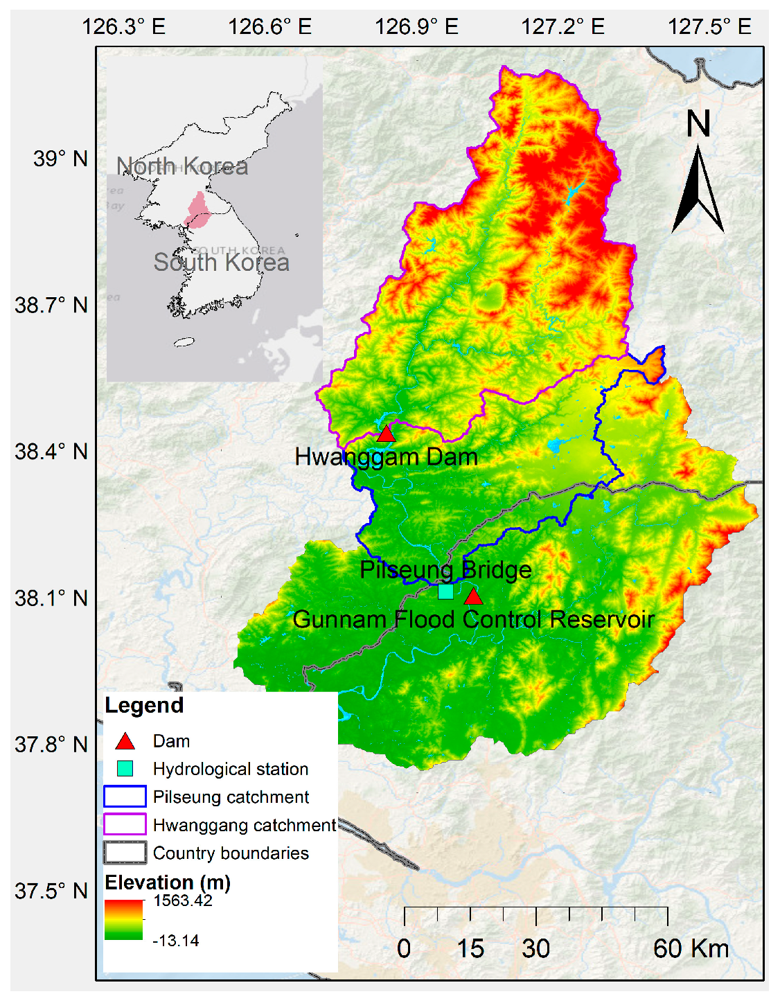
2. Study Area and Data

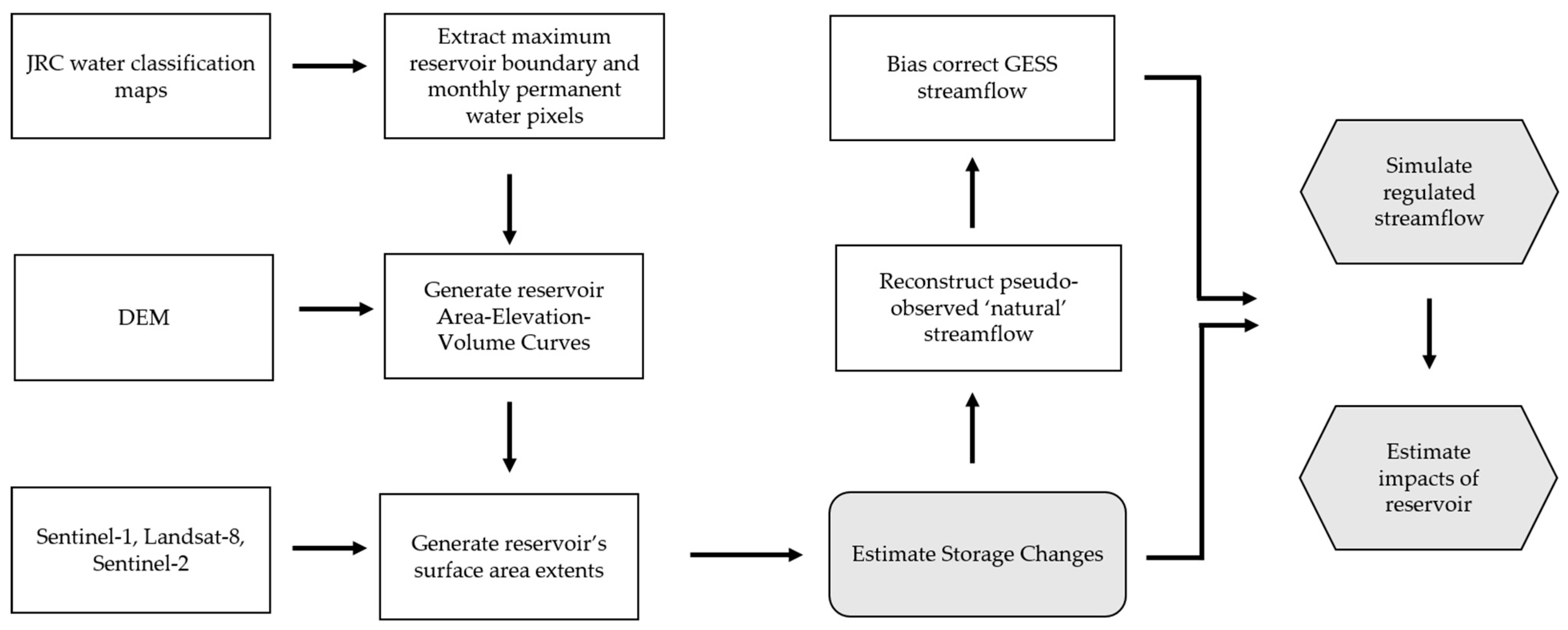
Since the division of North and South Korea, following the Korean War in 1953, the relations between the two countries have been stressed [29]. On the Korean Peninsula, the Imjin River is a transboundary river that flows from North Korea into South Korea (Figure 1). North Korea accounts for approximately two-thirds of the total watershed area of 8117 km². The Imjin river basin receives an average annual precipitation of around 1100 mm, of which the highest rainfall recorded in an hour is 120 mm [30]. About 74% of the total annual discharge takes place between June and September [29]. The construction of water infrastructure, such as the dams in North Korea upstream of the Imjin River, directly affects the downstream regions in South Korea. Unilateral actions taken by North Korea without coordination or agreement with South Korea, such as diversion to other basins and control of water release from the Hwanggang dam, which was built in 2007, are believed to have caused flood damage and water shortages in the downstream section of the Imjin River in South Korea. The Hwanggang dam, the largest multi-purpose dam in the Imjin River, is located on the upper stream of the Imjin River, 42.3 km north of the demilitarized zone (DMZ). Its reservoir capacity is estimated to be between 300 and 400 million m³ [31].

Since the information about dams in North Korea is highly limited, we used alternative data sources for monitoring reservoir dynamics, as shown in

Table 1. Data information in this study.

Purpose	Variable	Products	Duration	Spatial Resolution	Temporal Resolution	Reference
Estimate reservoir operation	Water surface area	Sentinel-1 SAR Ground Range Detected (GRD) imagery	2016–2021	10 m	6–12 days	[33]
		Sentinel-2	2019–2021	10 m	5–10 days	[40]
		Landsat-8	2016–2021	30 m	16 days	[41]
		Joint Research Centre (JRC) Global Surface Water Mapping Layers v1.4	1984–2021	30 m	Monthly	[11]
	Area–Elevation–Volume Curves	Shuttle Radar Topography Mission (SRTM) Digital Elevation Models (DEMs)	2002	30 m		[38]
Reconstruct pseudo-observations		In situ streamflow data at Pilseung	2011–2021		Daily
Estimate streamflow	Streamflow	GEOGLoWS ECMWF Streamflow Services (GESS)	1979–2021		Daily *	[27]
Characterize climate conditions	Precipitation	Global Precipitation Measurement Integrated Multi-SatellitE Retrievals for GPM (GPM-IMERG) and	2001–2021	0.1°	Daily	[34]
	Temperature	European Centre for Medium-Range Weather Forecasts (ECMWF) fifth-generation reanalysis product (ERA5)	1979–2021	0.25°	Daily	[35]

* Daily data was averaged from hourly data.

. Google Earth Engine (GEE) was used to retrieve and process remote sensing imagery (GEE; [32]). In order to obtain the reservoir boundary, the European Commission’s Joint Research Center’s (JRC) 38-year water mapping product was used [11]. Multi-sensor remote sensing imagery, including Landsat-8, Sentinel-2, and Sentinel-1 Synthetic Aperture Radar (SAR) Ground Range Detected (GRD) imagery, were used to derive the surface extents of the reservoir [33]. The monthly climatology of precipitation and temperature obtained from the Global Precipitation Measurement (GPM) Integrated Multi-Satellite Retrievals for GPM (GPM-IMERG) final product [34] and the European Centre for Medium-Range Weather Forecasts (ECMWF) fifth-generation reanalysis product (ERA5) [35] were used to characterize climate conditions in our study region. The temporal resolution of the computed reservoir water storage changes can be as high as one day by using this suite of sensors. Although SAR can illuminate the target under any weather conditions [36], it is less effective in mapping dry snow using the typical backscattering threshold-based approach [37]. With snow in the study area during winter, optical imagery was used to better detect water and snow. The SRTM DEM [38,39] was used to determine the area–elevation–volume (AEV) relationship of the reservoir behind the dam. With a mean absolute error of 2.49 m for 46 lakes and reservoirs in the United States, it was shown that the SRTM DEM provided adequate hydro-flattened surfaces for tracking lake surface elevations [16]. By combining the AEV relationship with the time series of surface water areas, reservoir elevations, volumes, and storage changes can be estimated [14,15]. GESS was used to simulate inflow into the reservoir. The daily observed streamflow data at Pilseung Bridge in South Korea (Figure 1) were collected to reconstruct natural discharge at the Hwanggang dam and to validate the simulated streamflow from GESS. These data were available from 2011 to the current date, and were provided by K-water.

3. Methods

To conduct this study, we followed three key steps: (1) estimating reservoir storage changes using remote sensing data; (2) reconstructing pseudo-observations using historical observed discharge; and (3) using GESS and satellite-based reservoir storage changes to estimate reservoir dynamics and regulated streamflow, as shown in Figure 2.

3.1. Using Remote Sensing Imagery to Compute Reservoir Storage Changes

To compute satellite-based storage changes, this study adopted the approach from Du et al. [14]. The following steps explain the methodology in more detail.

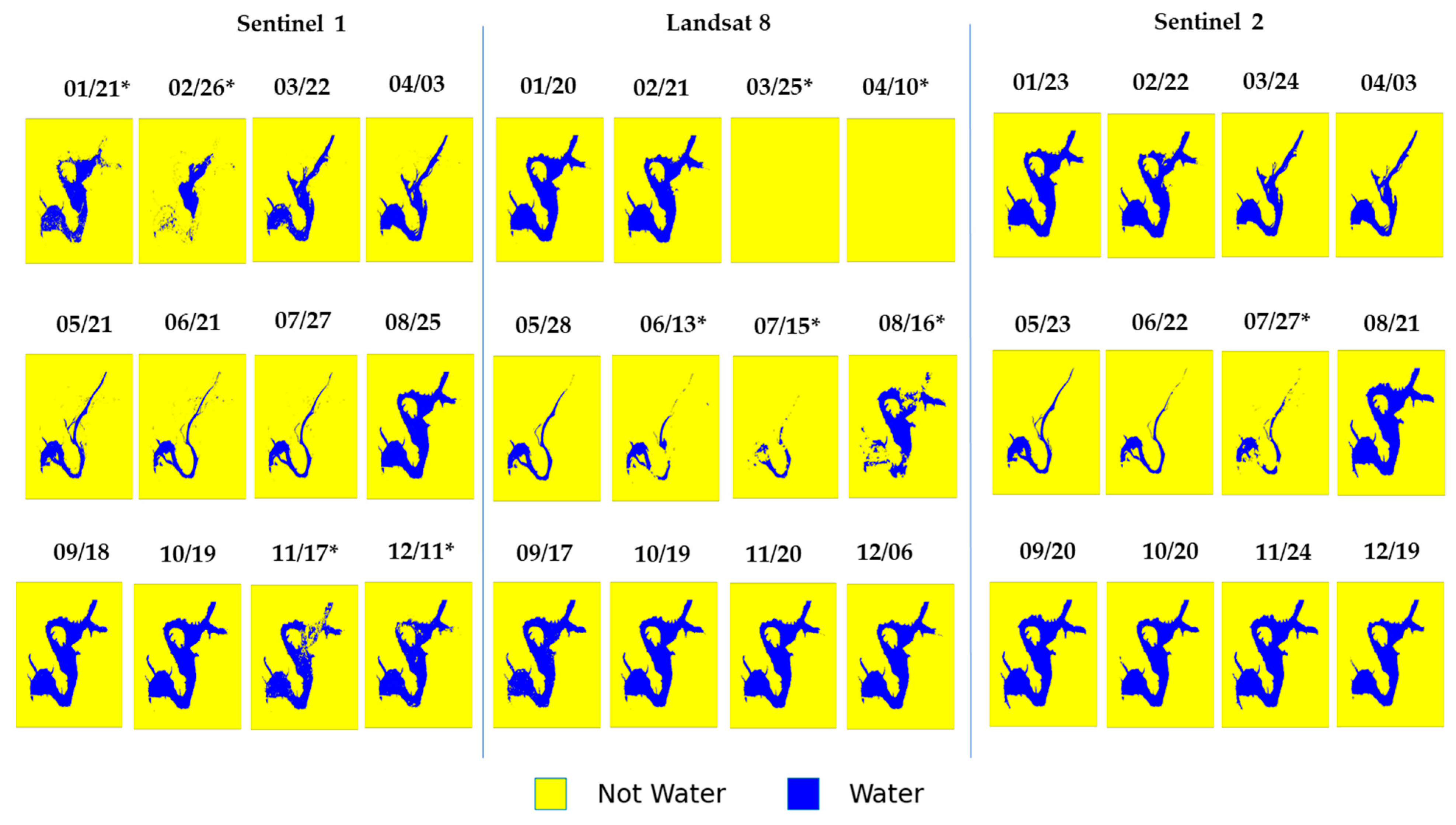
3.1.1. Identifying Reservoir Boundary

Identifying the boundaries of a reservoir is the first step in obtaining AEV relationships from DEM and in precisely estimating the surface areas of the reservoir for all the available satellite image acquisition date (i.e., by summing up water pixels within the determined boundary). To do this, a square polygon covering the reservoir was drawn from a center coordinate of the target reservoir, as identified on a GEE base map. Within this polygon, the JRC water classification, which covers the period of 1984 to 2021, was used to identify the maximum water occurrence for each pixel, with a resolution of 30 m [14]. To determine the maximum extent of the reservoir, the largest group of connected water pixels that intersect with the center coordinate of the target reservoir was extracted. As reservoir boundaries can change seasonally, it is important to identify the peak-season state of reservoir operation. To achieve this, a maximum reservoir extent was defined by masking out the non-water pixels throughout the multi-decadal history of water classification.

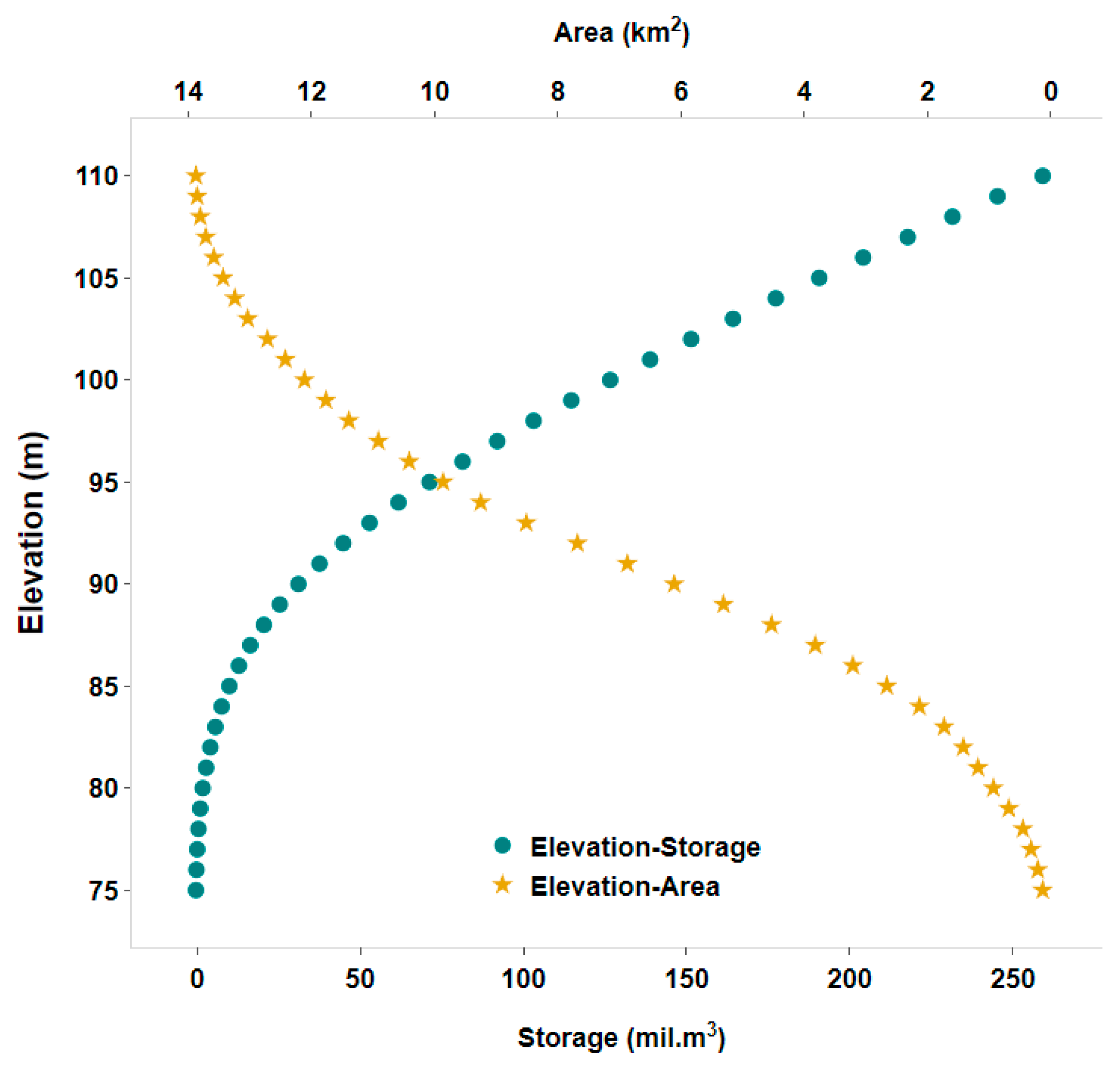
3.1.2. Generating Reservoir Area–Elevation–Volume Curves

The elevation data extracted from the SRTM DEM was used to calculate the surface area of each 1 m interval of elevation. This allowed estimation of the relationship between reservoir elevations and areas (E–A) within the border of the maximum reservoir extent. If underwater topography was not identified, a simple linear interpolation was fitted to the lower E–A relationship for each reservoir to estimate the E–A relationship below the hydro-flattened water levels from the SRTM DEM; the data were collected in February of 2000. The corresponding reservoir volumes (V) at each elevation interval (i) were then calculated using a trapezoidal approximation (Equation (1)), where A_i and h_i represent area and water elevation at the ith band of the E–A curve, respectively. V_i is the sum of all storage volumes accumulated from the lowest elevation band to the ith band. n is the total count of elevation intervals within the reservoir boundary.

$$V_i=\sum _{i=1}^n\frac{{\left(A_i+A_{i-1}\right)(h}_i-h_{i-1})}{2}$$

(1)

3.1.3. Estimating Reservoir Storage Changes

For optical imagery from Sentinel-2 and Landsat-8, the Modified Normalized Water Index (MNDWI) was estimated at cloud-free pixels (i.e., cloud coverage pixels less than 10%) [42]. The index is calculated using the green band (Band 3 of Landsat-8 and Sentinel-2) and the short-wave infrared (SWIR) band (Band 6 and Band 11 of Landsat-8 and Sentinel-2, respectively). The formula used for calculating the index is MNDWI = (X_green − X_swir)/(X_green + X_swir), where X is the reflectance value in the green or SWIR band. As water has relatively low reflectance in the SWIR region and high reflectance in the green region of the electromagnetic spectrum, higher values of MNDWI indicate a higher likelihood of water presence. Meanwhile, for Sentinel-1 SAR imagery, as different objects and materials reflect the SAR signal back to the sensor differently, the analysis of backscatter signatures allows for the differentiation between types of objects or materials [43]. Smooth open-water surfaces, characterized by their specular reflection properties, exhibit low backscatter values. The backscattering coefficients are normalized dimensionless numbers measuring the strength of radar signals reflected by the target object, and are expressed in dB. To reduce radar speckle noises in SAR imagery, a median filter was initially applied [36,44]. Then, the Edge Otsu method was utilized to identify the segmentation threshold for each image collection (i.e., Landsat-8, Sentinel-2, Sentinel-1) during the study period [45,46]. Once the segmentation threshold was established, pixels were classified as water if dB values were below the threshold for Sentinel 1 images, or if MNDWI values were above the threshold for Sentinel-2 and Landsat 8 images.

To identify image acquisition dates with inaccurate estimations of reservoir surface areas due to cloud or snow cover, the minimum water pixels for each month was determined using the JRC water classification maps. Within the previously identified maximum reservoir boundary, permanent water pixels were identified for each month based on their historical water occurrences. Specifically, water pixels were considered permanent if they had occurred in more than 90% of all available JRC water classification images during the same month since the commission of the reservoir. The classified water images obtained by using the threshold segmentation were then filtered to retain only those that intersected with the minimum water pixels of the respective month. For those retaining images, the reservoir’s surface areas were determined by summing up the water pixels within the maximum reservoir boundary.

Since the temporal resolution of multi-sensor imagery is between 1 and 16 days, the time series of daily surface areas were created by linearly interpolating the remote sensing-based reservoir areas for the complete period from January 2016 to December 2021 (the specific equations for this interpolation can be found in Equation (S1)). To reduce other uncertainties due to sensor and water-mapping errors, before interpolation, a 5-day weighted moving average was applied. The associated reservoir elevations and storage volumes were determined by linking the reservoir AEV relationship with the time series of reservoir areas (more details can be found in Equation (S2)). By subtracting the storage volume of the day before from the storage volume of the target day, reservoir storage changes ($∆S$) for each target day were calculated.

3.2. Reconstructing Pseudo-Observations at Hwanggang Dam and Pilseung Bridge before and after Dam Operation

Since GESS only considers the natural process of surface- and subsurface-runoff generation from meteorological forcing, simulated streamflows only represent “natural” flows. Meanwhile, observed streamflow data at Pilseung bridge (Figure 1), located approximately 40 km downstream of the dam, are available from 2011 onward. As the operation of the Hwanggang dam commenced in 2007, there are no observed data in the “natural” condition before the dam’s operation. To evaluate the simulated streamflow from GESS at both locations before and after the dam’s operation, we generated additional observations by reconstructing the data based on actual observed data at Pilseung bridge. The reconstructed data are referred to as “pseudo-observations”. “Natural” streamflow data was reconstructed under an assumption that the daily storage changes estimated from remote sensing imagery were accurate. We also assumed that the topography and climate conditions generating streamflow at both locations were the same, except for their drainage areas, for reconstructing the observations at the Hwanggang dam. Validation of the satellite-based storage changes was visually undertaken and is shown in Section 4.1. The reconstructed pseudo-observations ($Q_{pseudo-obs}$) included inflows ($Q_{in}$), and outflows ($Q_{out}$) of the Hwanggang reservoir, and the “natural” streamflow at Pilseung bridge ($Q_{nat}$).

Consequently, we estimated the “natural” streamflow $\left(Q_{nat}\right)$ at Pilseung bridge using the in situ data at Pilseung $\left(Q_{obs}\right)$ and the satellite-based storage changes of the Hwanggang dam ($∆S$) estimated from step 3.1.3, as shown in Equation (2).

$$Q_{nat}=Q_{obs}+∆S$$

(2)

The pseudo-observed reservoir inflows into the Hwanggang dam ($Q_{in})$ were estimated by multiplying the drainage ratio between two catchments with the “natural” streamflow at Pilseung bridge $\left(Q_{nat}\right),$ as displayed in Equation (3). The drainage ratio ($ratio$) between the two catchments was computed using upstream drainage area variables from the Multi-Error-Removed-Improved-Terrain (MERIT) Hydro datasets [47]. In this study, as the drainage areas of the Hwanggang dam and Pilseung are 2693.384 km² and 4108.974 km², the drainage ratio was calculated as 0.65.

The Hwanggang dam outflows ($Q_{out})$ were then calculated as the difference between the Hwanggang dam inflows ($Q_{in})$ and the satellite-based storage changes ($∆S$) (Equation (4)). Although the simulated streamflow from GESS considers the evaporation in the upstream catchment area, evaporation from the reservoir is not considered. Here, we assumed that $∆S$ included both the changes due to reservoir releases/storages and to evaporation.

$$Q_{in}=Q_{nat}\times ratio$$

(3)

$$Q_{out}=Q_{in}-∆S$$

(4)

3.3. Estimating and Evaluating Regulated Streamflows at Hwanggang Dam and Pilseung Bridge

To obtain the simulated streamflow ($Q_{GESS-raw})$ from GESS, we first identified their GESS reach IDs (i.e., Hwanggang dam: 4040202, Pilseung bridge: 4041153). Like other GHMs, GESS has biases in its simulation due to various factors such as errors in input data, model structure, and parameterization. The bias correction is a technique used to adjust the model estimates to reduce these biases and improve their accuracy. To do so, in this study, the quantile mapping approach by Farmer et al. [24] was used to correct the bias of GESS streamflow under “natural” conditions ($Q_{GESS-corrected}$). Quantile mapping was chosen because of its simplicity and ability to maintain variability in the model’s output distribution while adjusting for consistent biases [24,48,49]. Bias correction involves comparing the cumulative distribution functions (CDFs) of the simulated streamflow ${(Q}_{GESS-raw})$and the pseudo-observed reservoir inflows into the Hwanggang dam ($Q_{in})$ during overlapping historical periods. Discrepancies between the two distributions are indicative of biases, where the model may consistently overestimate or underestimate streamflow values. By identifying specific quantiles along the distribution where these discrepancies are the most pronounced, the quantile mapping approach guides the adjustment process. Subsequent adjustments target specific quantiles in the new simulated streamflow data, aiming to reduce the biases while maintaining the overall shape and variability of the model’s output. The mass balance (MB) approach, which combines the corrected historical inflows and the interpolated daily satellite-based storage changes, was subsequently used to obtain the simulated Hwanggang dam outflows and the regulated streamflow at Pilseung bridge ($Q_{GESS-reg}$), as shown in equation 5.

$$Q_{GESS-reg}=Q_{GESS-corrected}-∆S$$

(5)

Four metrics were used to evaluate the agreement between the simulated GESS streamflow ($Q_{GESS-raw}{,Q}_{GESS-corrected},Q_{GESS-reg}$) and the observations (

Table 2. Performance metrics adopted in this study.

Statistical Metrics	Formulas	Optimal Values
Relative Error (RE)	$RE=\frac{\overline{Q_{sim}}-\overline{Q_{obs}}}{\overline{Q_{obs}}}\times 100$	−25% to 25%
Relative Error of Standard Deviation (RESD)	$RESD=\frac{S_{Qsim}-S_{Qobs}}{S_{Qobs}}\times 100$	−25% to 25%
Pearson’s Correlation Coefficient (CC)	$CC=\frac{\sum \left(Q_{obs}-\overline{Q_{obs}}\right)\left(Q_{sim}-\overline{Q_{sim}}\right)}{\sqrt{\sum {\left(Q_{obs}-\overline{Q_{obs}}\right)}^2\sum {\left(Q_{sim}-\overline{Q_{sim}}\right)}^2}}$	0.5 to 1
Kling–Gupta Efficiency (KGE)	$KGE=1-\sqrt{{\left(CC-1\right)}^2+{\left(\frac{S_{Qsim}}{S_{Qobs}}-1\right)}^2+{\left(\frac{\overline{Q_{sim}}}{\overline{Q_{obs}}}-1\right)}^2}$	0 to 1

where $S_{Qobs}$ and $S_{Qsim}$ are standard deviations of observed ($Q_{obs}$) and simulated streamflow ($Q_{sim}$), respectively; $\overline{Q_{sim}}$ and $\overline{Q_{obs}}$are averages of observed and simulated streamflow, respectively.

). It should be noted that the only available ground observations were those of the regulated streamflow at Pilseung bridge, while the remaining data were reconstructed pseudo-observations, as described in Section 3.2. The error metrics included the Kling–Gupta efficiency (KGE) and its components (Pearson’s correlation coefficient (CC), relative error (RE), and relative error of standard deviation (RESD) [50,51]. They were used to decompose and comprehend the error components.

3.4. Estimating Hydrological Impacts of Hwanggang Dam

The Hwanggang Dam serves multiple purposes such as irrigation, flood control and hydropower generation [36]. It has also been purportedly used as a geopolitical tool against the South Korean government. Communities downstream of the Hwanggang Dam in both North and South Koreas depend on the Imjin River for aquaculture and rice cultivation [52]. Consequently, any mismanagement of dam operations can adversely affect the farming communities in both nations and disrupt the power generation in North Korea. To assess the hydrological impacts of the Hwanggang dam, we calculated the median monthly percentages of reservoir storage changes compared to “natural” streamflow at both the Hwanggang dam and Pilseung bridge catchments. Additionally, we investigated whether the regulated streamflow increased or decreased the percentage of daily extreme-high and -low flows for each month compared to the “natural” streamflow. To achieve this, we first estimated the monthly “natural” streamflow quantile thresholds at the 99th percentile (i.e., extreme-high flows or floods) and the 1st percentile (i.e., extreme-low flows or water shortages) from 2016–2021. Then, we computed the percentage of daily regulated and “natural” streamflow exceeding or below the thresholds for each month. By comparing the differences, we can discern the impacts of reservoir operation on the occurrence of extreme flow events.

4. Results and Discussion

4.1. Estimating Reservoir Storage Changes Using Remote Sensing

4.1.1. Reservoir Area–Elevation–Volume (AEV) Curves

As shown in Figure 3, the AEV curve of the Hwanggang dam was derived using the SRTM DEM and trapezoidal formula as explained in Section 3.1.2. To identify underwater topography at ungauged locations, Yigzaw et al. [53] used dam height information to identify the lowest elevation of reservoirs. Meanwhile, Biswas et al. [15] applied a linear interpolation method to fit E–A curves to determine the minimum elevation at which the cumulative surface area becomes zero. Given the absence of dam height information at the Hwanggang dam and negligible bias between lowest elevation derived from the linear fit and that from the existing E–A curves of the SRTM DEM, we did not apply a linear fit for the E–A curves. Instead, we directly utilized data from SRTM. In the study by Kim et al. [36], an elevation of 110 m was estimated to correspond to an area of 15 km², while in the study by JG Kim et al. [54], it corresponds to 12 km². In our study, the elevation of 110 m corresponded to an area of 14 km², which is closer to that of Kim et al. [36], which used the SRTM DEM as well (Figure 3).

4.1.2. Reservoir Storage Changes

When direct observational data are absent due to inevitable circumstances, cloud-free optical imagery often serves as “ground truth” [55]. In this study, cloud-free Landsat 8 and Sentinel 2 are the most reliable sources. However, we excluded certain months where images were compromised by partial or full cloud cover. To increase the temporal resolution of optical images, we supplemented optical imagery with SAR imagery, which ensures continuous observations under all-weather conditions [56]. Since this reservoir operates on a within-year basis due to its high storage ratio (i.e., calculated as the reservoir storage divided by annual inflow) of 0.2, its average surface area typically exhibits less sensitivity to daily storage fluctuations than the behaviors seen in run-of--river reservoirs [57]. Figure 4 shows the comparison of water pixels among Sentinel-1, Landsat-8 and Sentinel-2 images in 2019. If a day in the figure is accompanied by a star notation, that date image is filtered out because the water pixels did not overlap with permanent water pixels, as described in Section 3.1.3. The figure demonstrates that the classified water pixels from all three collections consistently agreed in mapping the dynamics of reservoir surface extents in snow- and cloud-free months. However, larger discrepancies in water pixels between Sentinel-1 and other optical images were found during the days with snow cover in December, January, and February (i.e., in these months temperatures are below freezing temperature, as shown in Figure 5). The presence of liquid water contents in wet or dry snow affects the scattering mechanisms recorded in SAR images. This characteristic can hinder the effectiveness of using the backscattering-based threshold approach in mapping snow-covered pixels, as concluded by previous studies [37,58,59,60,61]. Reservoir patterns, in this study, refer to the operational rules of reservoirs based on monthly average water levels and dam releases.

The total number of images that were not filtered out due to the water classification errors (i.e., not intersecting with minimum permanent pixels) were 224, 49, and 49 for Sentinel-1, Landsat-8 and Sentinel-2, respectively, from 2016 until 2021. While most of the remaining Landsat-8 and Sentinel-2 images were taken in dry months (i.e., September until May), the majority of retained Sentinel-1 images were captured during snow-free months (i.e., March until November) (Figure 4 and Figure 5 and Supplementry Figure S1). The time series of monthly climatology of precipitation and temperature confirmed that the region typically receives more precipitation from May to September and has freezing temperatures from December to February (Figure 5). Although Landsat-8 images were available before 2016, this study focused on the period after 2016 when Sentinel-1 became available to maximize the number of publicly available images for a better understanding of reservoir operation patterns. Figure 5 illustrates that the surface areas of the reservoir often increase during wet months from May to September for water storage, remain relatively stable during snowy months from November to January, and then decrease from February to April due to evaporation, snowmelt, or water release. Beyond the seasonal fluctuations in reservoir areas over the years, we also noticed that maximum reservoir sizes vary annually based on the region’s total annual precipitation. A strong positive correlation exists between the peak reservoir areas (or maximum storage capacities) and the annual precipitation. Reduced reservoir areas were noted during dry years, specifically in 2019, 2021, and 2022. Conversely, 2020, a year marked by flooding with an extra 50% precipitation, witnessed exceptionally high reservoir areas (see Figure 5).

Although a reservoir operation can increase water availability in the dry season and help control floods in the flood season, mismanagement of such dam operation [62,63] and militarization of dams [64] can cause catastrophic impacts on downstream residents. In the case of the Hwanggang dam, on 6th September 2009, the fifth water conflict was believed to have been caused by North Korea’s unexpected water releases, since there was no rainfall in the Hwanggang Reservoir catchment at that time [65]. Without any prior warning, North Korea allegedly released approximately 40 million tons of water between 2:00 a.m. and 1:00 p.m. on 6th September 2009 (11 h) [66]. As a result, six citizens tragically died of the flash flood that happened in South Korea downstream of the Imjin River, although it must be stated that there was no data-driven evidence to support the claims.

Accordingly, in our study, to evaluate the impacts of the Hwanggang reservoir operation objectively on downstream hydrology, it is important to understand its hydrology as if there were no operating reservoirs. If there is suddenly heavy rain driving high water inflows that exceed the reservoir capacity, the sudden release of the reservoir is due to local weather conditions rather than the reservoir itself. Nonetheless, since the temporal resolution of the reservoir surface areas is not daily but 1-to-16 days, the interpretation of reservoir dynamics should be carried out with caution, as it might not appear as a sudden increase or decrease, but with gradual changes.

4.2. Estimating Streamflow Using the Publicly Available Global Hydrological Model and Satellite-Based Reservoir Storage Changes

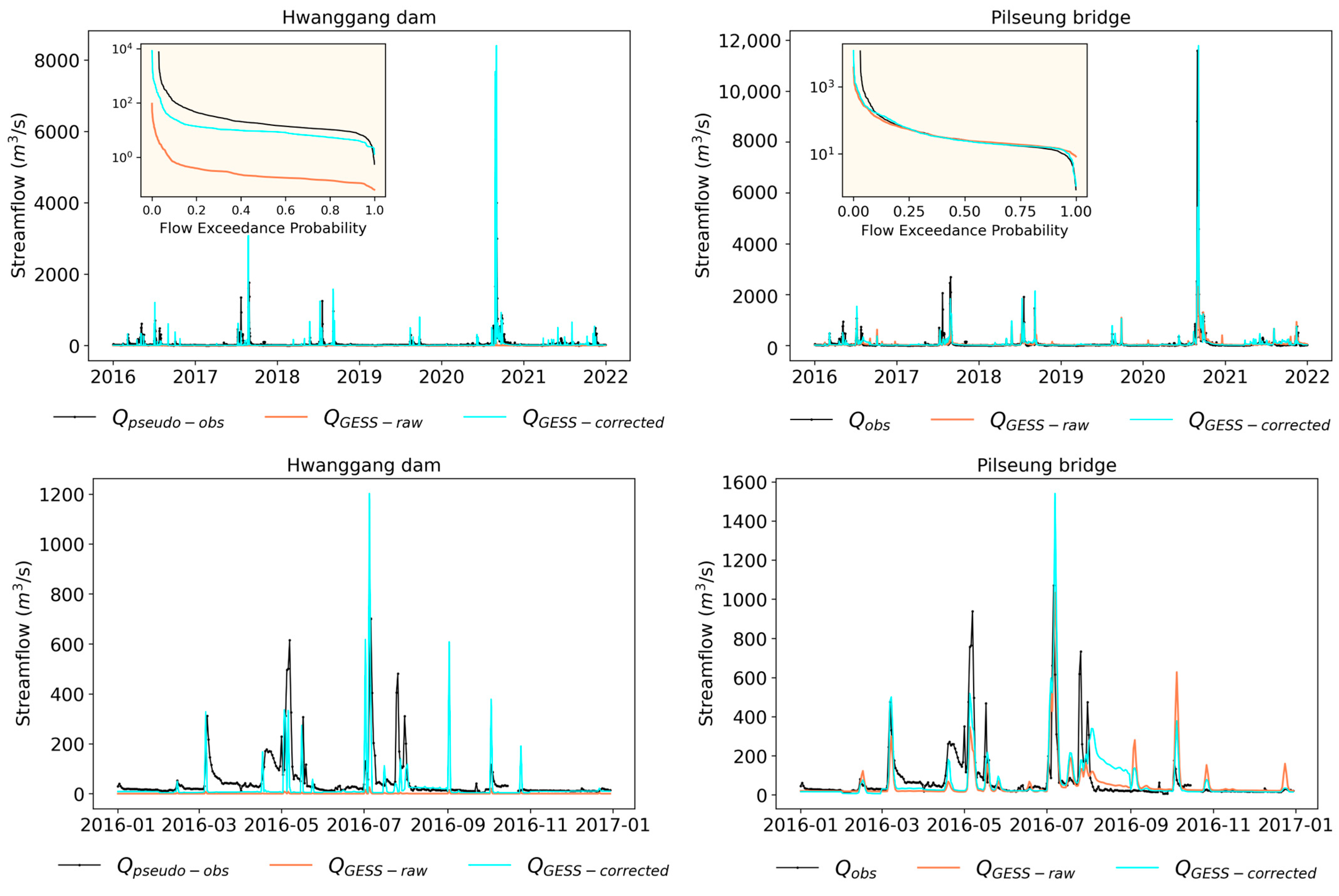
4.2.1. Estimating Streamflow in “Natural” Conditions

Results from global hydrologic models frequently exhibit biases, as the models often use a single parameter set globally, which can have a substantial impact on the accuracy of a hydrological event simulation and limit the usage of the model. Bias correction like quantile mapping has been found to effectively reduce the volume bias of simulated streamflow [26,67].

The performance of GESS streamflow without reservoir operation is illustrated in Figure 6 and

Table 3. Statistical evaluation of GESS streamflows before ($Q_{GESS-raw}$) and after bias correction ($Q_{GESS-corrected}$) compared to the pseudo-observed data ($Q_{pseudo-obs}$) at the Hwanggang dam and Pilseung bridge.

Temporal Scale	Variables	CC	KGE	RE	RESD
Daily scale	Hwanggang $Q_{GESS-raw}$	0.37	−0.53	−98.64%	−98.67%
	Hwanggang $Q_{GESS-corrected}$	0.41	0.33	−28.14%	12.10%
Monthly scale	Hwanggang $Q_{GESS-raw}$	0.98	−0.40	−98.64%	−99.01%
	Hwanggang $Q_{GESS-corrected}$	0.98	0.70	−28.98%	−7.58%
Daily scale	Pilseung $Q_{GESS-raw}$	0.74	0.41	−14.56%	−51.92%
	Pilseung $Q_{GESS-corrected}$	0.72	0.68	14.50%	1.80%
Monthly scale	Pilseung $Q_{GESS-raw}$	0.95	0.54	−14.17%	−43.25%
	Pilseung $Q_{GESS-corrected}$	0.98	0.75	14.69%	20.59%

. From Figure 6, the bias-corrected GESS streamflow ($Q_{GESS-corrected}$) overall agrees better with the reconstructed “natural” streamflow ($Q_{pseudo-obs}$) at both the Hwanggang dam and Pilseung bridge than with the uncorrected streamflow ($Q_{GESS-raw}$). Graphs of flow-duration curves are also included in Figure 6. While the bias correction significantly improved the simulation of GESS at Hwanggang dam, it slightly improved the simulation GESS at low flows (inset figures of Figure 6). In terms of statistical metrics, the bias correction significantly improved the volume-bias and variability-bias components of the KGE metrics at Hwanggang dam on a daily scale (i.e., KGE changes from −0.53 to 0.33, RE changes from −98.64% to −28.47%, and RESD from −98.67% to 12.10%, after bias correction). Similarly, at Pilseung bridge, on the daily scale, KGE improved from 0.41 to 0.68, with most of changes driven by the reduction in the variability bias from −51.92% to 1.80%. On the monthly scale, KGE at both locations was above 0.7. The positive KGE is considered as indicative of “good” model simulations [51]. Future research could incorporate ensemble streamflow simulations from various GHMs to mitigate uncertainties associated with a single global universal parameter set of one model [68].

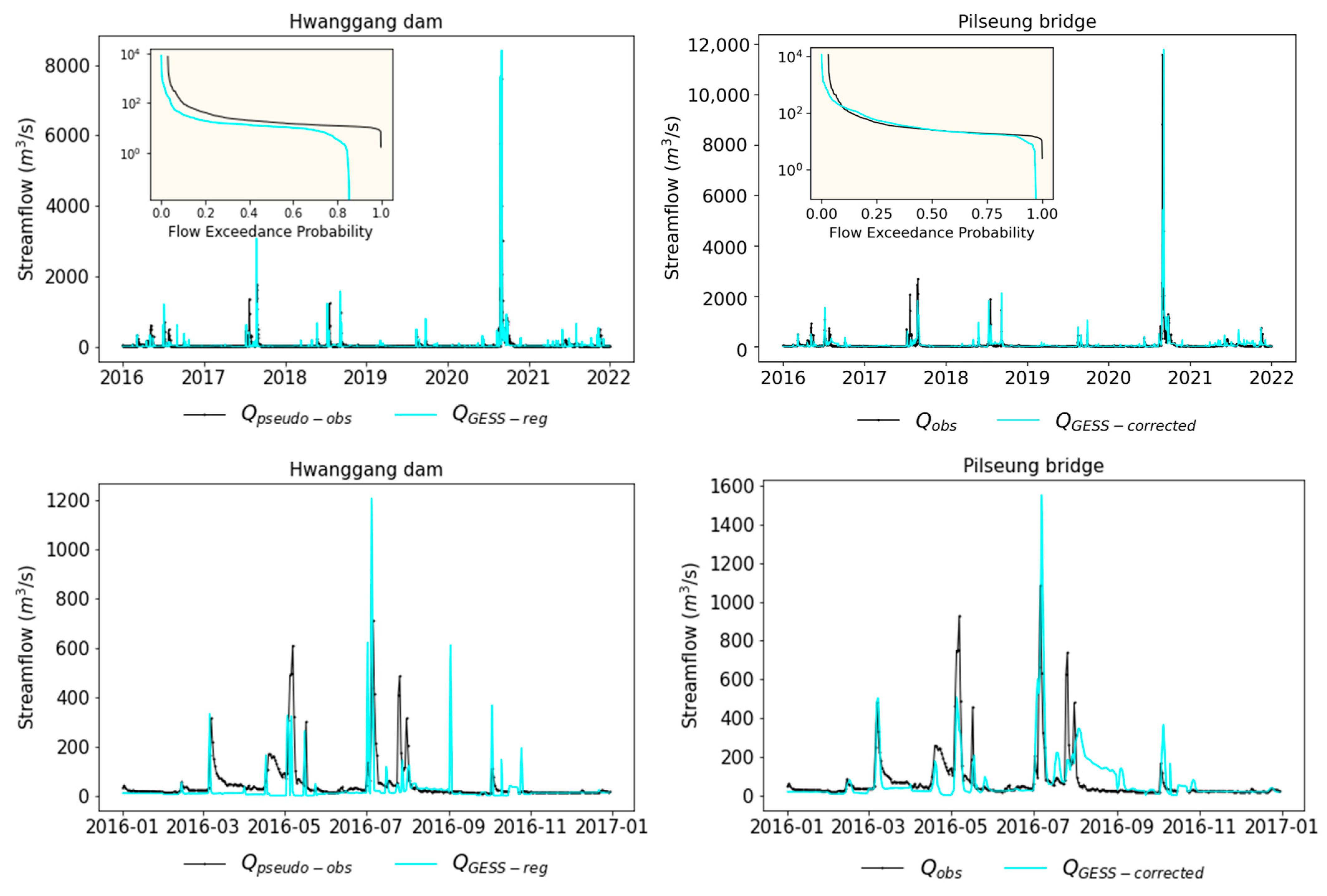
4.2.2. Estimating Streamflow in Regulated Conditions

Figure 7 and

Table 4. Statistical evaluation of GESS-simulated regulated streamflow ($Q_{GESS-reg}$) compared to pseudo-observed data ($Q_{pseudo-obs}$) at the Hwanggang dam and actual observed data ($Q_{obs}$) at Pilseung bridge.

Temporal Scale	Variables	CC	KGE	RE	RESD
Daily scale	Hwanggang $Q_{GESS-reg}$	0.41	0.34	−26.17%	12.19%
	Pilseung $Q_{GESS-reg}$	0.72	0.67	15.82%	1.88%
Monthly scale	Hwanggang $Q_{GESS-reg}$	0.97	0.75	−23.63%	−7.48%
	Pilseung $Q_{GESS-reg}$	0.98	0.73	17.55%	20.68%

show the hydrographs and performance of regulated streamflow at the Hwanggang dam and Pilseung bridge. The KGE metrics for both the Hwanggang dam and Pilseung bridge were 0.34 and 0.67, respectively, on a daily scale, and 0.75 and 0.73, respectively, on a monthly scale. As the simulation of inflow at the Hwanggang dam had a low temporal correlation of 0.41, the simulated outflow also resulted in a low correlation of 0.41. Future studies can incorporate the hydrological model setup and integrated reservoir operation scheme (IROS) for better modelling of regulated streamflow due to reservoir operation [14]. Nevertheless, the use of a global hydrological model with the bias correction and satellite-based storage changes can provide useful insights for understanding hydrological regimes and the reservoir operation patterns at ungauged locations, especially when there are limited data availability and restricted modeling resources.

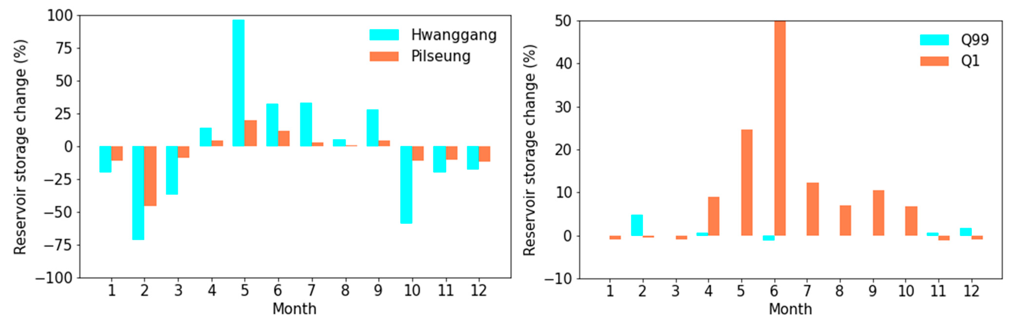
4.3. Estimating Hydrological Impacts of Reservoir Operation

The median monthly percentage of Hwanggang storage changes compared to the simulated “natural” streamflows at the Hwanggang dam and Pilseung bridge ($Q_{GESS-corrected}$) are shown in Figure 8. A negative percentage often indicates the loss of storage due to evaporation, snowmelt, or reservoir release, while a positive percentage indicates an increase in reservoir storage. In Figure 8, the median monthly percentage of reservoir storage is positive in the wet months (i.e., from April to September) and negative in the dry months (i.e., October until March). In particular, the median monthly percentage of reservoir storage exceeded 90% in May, since the median monthly simulated “natural” streamflows were equivalent to the reservoir storage changes occurring at the Hwanggang dam (Figure S2). The overall changes were higher at the Hwanggang dam catchment of North Korea, than at the Pilseung bridge catchment of South Korea (i.e., the median percentages across all months were 30% and 11% in the Hwanggang dam and Pilseung bridge, respectively).

Additionally, to understand the impacts of the Hwanggang dam on the downstream catchment in South Korea, particularly at Pilseung bridge, the differences in percentage of monthly regulated streamflow and natural streamflow exceeding or below the monthly streamflow quantile thresholds at 99% (i.e., Q99 or likelihood of flood events) and 1% (i.e., Q1 or likelihood of water shortage events) were calculated for each month in the period of 2016–2021. The findings indicate that the Hwanggang dam had minimal impact on flooding, likely due to its low level of regulation (30% at the Hwanggang dam catchment and 11% at Pilseung bridge catchment) while it slightly reduced the likelihood of water shortages during low-precipitation months (i.e., from November to February). However, it was likely to increase the probability of wet-month water shortages due to the reservoir storage, particularly in June. It is important to note that the analysis was limited to a short period of six years due to the available overlapping period of all remote sensing images used in the study. If there were available remote sensing imagers passing the reservoir over a disputed event in the future, a closer examination using the proposed approach of publicly available data from the study could be used to provide information necessary to prevent conflict escalation. The proposed methodology incorporating a global hydrological model and remote sensing imagery in ungauged basins can, therefore, have the potential to provide valuable insights for decision-makers to collaborate with upstream countries in resource allocation and mitigate geopolitical conflicts, thereby preventing significant negative impacts on downstream communities.

In particular, when the agricultural activities downstream are mainly rice cultivation and aquaculture [52], and the main negative impacts from reservoirs are mostly water shortage, the study’s findings highlight the need for increased mitigation and adaption efforts to address human-induced drought impacts. Currently, the Gunnam Flood Control, located downstream of the Pilseung Bridge station in South Korea (Figure 1) with a storage capacity of about 71 million cubic meters [69], serves primarily for flood control. However, this reservoir can be repurposed as an irrigation storage pond during months vulnerable to reservoir-induced droughts [70]. Alternatively, adapting agricultural practices could be implemented. This might involve switching crop types in response to seasonal climate forecasts [71]. Moreover, given the transboundary nature of the Imjin River basin, the sharing of hydrological data, weather forecasts, and other relevant information is vital. A recommended approach is to initiate negotiations and dialogues to coordinate a dam release which is beneficial for farming communities in both countries [72]. Should these measures prove inadequate, compensations methods (e.g., resettlement and financial reparations) offer a viable strategy to safeguard those adversely affected by reservoir operation risks [73,74].

5. Conclusions

This study highlights the fact that publicly accessible global hydrological models and satellite-based reservoir storage changes can provide useful information at ungauged reservoirs and basins to develop effective plans for transboundary water resource management. The potential of remote sensing imagery for monitoring reservoir operation in transboundary basins has been demonstrated in numerous studies. Previous studies, nevertheless, have not examined whether a global hydrological model without direct calibration in the local watershed can be used to understand the impacts of reservoir operation on downstream hydrology. The study found that a publicly accessible global hydrological model, such as the GESS platform, when combined with bias correction, can provide acceptable streamflow simulation at ungauged locations. Although the bias correction technique using quantile mapping successfully alleviated biases in streamflow predictions from the GESS model, both on a daily and monthly basis, its skill in enhancing daily temporal correlation is still limited. However, this approach presents a rapid and cost-effective alternative to initiating the lengthy and data-intensive process of setting up a catchment model. The model’s monthly simulations, with KGE and CC values exceeding 0.7 for both metrics, confirm the robustness of the proposed methodology. We conclude that integrating bias-corrected streamflow simulation and satellite-based storage changes can provide important insights into reservoir operation patterns and their impacts for efficient resource allocation that consequently reduce the negative impacts on downstream communities.

References

1. ICOLD CIGB > General Synthesis. Available online: https://www.icold-cigb.org/GB/world_register/general_synthesis.asp (accessed on 16 January 2023).
2. De Stefano, L.; Petersen-Perlman, J.D.; Sproles, E.A.; Eynard, J.; Wolf, A.T. Assessment of transboundary river basins for potential hydro-political tensions. Glob. Environ. Change 2017, 45, 35–46. [Google Scholar] [CrossRef]
3. Gleick, P.H.; Heberger, M. Water Conflict Chronology. In The World’s Water: The Biennial Report on Freshwater Resources; Gleick, P.H., Ed.; Island Press/Center for Resource Economics: Washington, DC, USA, 2014; pp. 173–219. [Google Scholar] [CrossRef]
4. Choe, S.-H. South Korea Demands Apology from North over Dam Incident. New York Times, 8 September 2009. [Google Scholar]
5. Fox, C.A.; Sneddon, C.S. Political Borders, Epistemological Boundaries, and Contested Knowledges: Constructing Dams and Narratives in the Mekong River Basin. Water 2019, 11, 413. [Google Scholar] [CrossRef]
6. You, L.; Li, C.; Min, X.; Xiaolei, T. Review of Dam-break Research of Earth-rock Dam Combining with Dam Safety Management. Procedia Eng. 2012, 28, 382–388. [Google Scholar] [CrossRef]
7. Kibler, K.M.; Biswas, R.K.; Juarez Lucas, A.M. Hydrologic data as a human right? Equitable access to information as a resource for disaster risk reduction in transboundary river basins. Water Policy 2014, 16, 36–58. [Google Scholar] [CrossRef]
8. Gerlak, A.K.; Lautze, J.; Giordano, M. Water resources data and information exchange in transboundary water treaties. Int. Environ. Agreem. Politics Law Econ. 2011, 11, 179–199. [Google Scholar] [CrossRef]
9. Okeowo, M.A.; Lee, H.; Hossain, F.; Getirana, A. Automated Generation of Lakes and Reservoirs Water Elevation Changes from Satellite Radar Altimetry. IEEE J. Sel. Top. Appl. Earth Obs. Remote Sens. 2017, 10, 3465–3481. [Google Scholar] [CrossRef]
10. Markus, T.; Neumann, T.; Martino, A.; Abdalati, W.; Brunt, K.; Csatho, B.; Farrell, S.; Fricker, H.; Gardner, A.; Harding, D.; et al. The Ice, Cloud, and land Elevation Satellite-2 (ICESat-2): Science requirements, concept, and implementation. Remote Sens. Environ. 2017, 190, 260–273. [Google Scholar] [CrossRef]
11. Pekel, J.-F.; Cottam, A.; Gorelick, N.; Belward, A.S. High-resolution mapping of global surface water and its long-term changes. Nature 2016, 540, 418–422. [Google Scholar] [CrossRef] [PubMed]
12. Tulbure, M.G.; Broich, M. Spatiotemporal dynamic of surface water bodies using Landsat time-series data from 1999 to 2011. ISPRS J. Photogramm. Remote Sens. 2013, 79, 44–52. [Google Scholar] [CrossRef]
13. Gao, H.; Birkett, C.; Lettenmaier, D.P. Global monitoring of large reservoir storage from satellite remote sensing. Water Resour. Res. 2012, 48, e2012WR012063. [Google Scholar] [CrossRef]
14. Du, T.L.; Lee, H.; Bui, D.D.; Graham, L.P.; Darby, S.D.; Pechlivanidis, I.G.; Leyland, J.; Biswas, N.K.; Choi, G.; Batelaan, O.; et al. Streamflow Prediction in Highly Regulated, Transboundary Watersheds Using Multi-Basin Modeling and Remote Sensing Imagery. Water Resour. Res. 2022, 58, e2021WR031191. [Google Scholar] [CrossRef] [PubMed]
15. Biswas, N.K.; Hossain, F.; Bonnema, M.; Lee, H.; Chishtie, F. Towards a global Reservoir Assessment Tool for predicting hydrologic impacts and operating patterns of existing and planned reservoirs. Environ. Model. Softw. 2021, 140, 105043. [Google Scholar] [CrossRef]
16. Das, P.; Hossain, F.; Khan, S.; Biswas, N.K.; Lee, H.; Piman, T.; Meechaiya, C.; Ghimire, U.; Hosen, K. Reservoir Assessment Tool 2.0: Stakeholder driven improvements to satellite remote sensing based reservoir monitoring. Environ. Model. Softw. 2022, 157, 105533. [Google Scholar] [CrossRef]
17. Beven, K.; Young, P. A guide to good practice in modeling semantics for authors and referees. Water Resour. Res. 2013, 49, 5092–5098. [Google Scholar] [CrossRef]
18. Nearing, G.S.; Kratzert, F.; Sampson, A.K.; Pelissier, C.S.; Klotz, D.; Frame, J.M.; Prieto, C.; Gupta, H.V. What Role Does Hydrological Science Play in the Age of Machine Learning? Water Resour. Res. 2021, 57, e2020WR028091. [Google Scholar] [CrossRef]
19. Du, T.L.; Lee, H.; Bui, D.D.; Arheimer, B.; Li, H.Y.; Olsson, J.; Darby, S.E.; Sheffield, J.; Kim, D.; Hwang, E. Streamflow prediction in “geopolitically ungauged” basins using satellite observations and regionalization at subcontinental scale. J. Hydrol. 2020, 588, 125016. [Google Scholar] [CrossRef]
20. Tran, T.-N.-D.; Nguyen, Q.B.; Vo, N.D.; Marshall, R.; Gourbesville, P. Assessment of Terrain Scenario Impacts on Hydrological Simulation with SWAT Model. Application to Lai Giang Catchment, Vietnam. In Advances in Hydroinformatics; Gourbesville, P., Caignaert, G., Eds.; Springer Nature: Singapore, 2022; pp. 1205–1222. [Google Scholar] [CrossRef]
21. Ahmed, Z.; Tran, T.N.D.; Nguyen, Q.B. Applying Semi Distribution Hydrological Model to Assess Hydrological Regime in Lai Giang Catchment, Binh Dinh Province, Vietnam; Capital University of Science and Technology: Islamabad, Pakistan, 2020. [Google Scholar]
22. Shortridge, J.E.; Guikema, S.D.; Zaitchik, B.F. Machine learning methods for empirical streamflow simulation: A comparison of model accuracy, interpretability, and uncertainty in seasonal watersheds. Hydrol. Earth Syst. Sci. 2016, 20, 2611–2628. [Google Scholar] [CrossRef]
23. Sood, A.; Smakhtin, V. Global hydrological models: A review. Hydrol. Sci. J. 2015, 60, 549–565. [Google Scholar] [CrossRef]
24. Farmer, W.H.; Over, T.M.; Kiang, J.E. Bias correction of simulated historical daily streamflow at ungauged locations by using independently estimated flow duration curves. Hydrol. Earth Syst. Sci. 2018, 22, 5741–5758. [Google Scholar] [CrossRef]
25. Bonnema, M.; Sikder, S.; Miao, Y.; Chen, X.; Hossain, F.; Ara Pervin, I.; Mahbubur Rahman, S.M.; Lee, H. Understanding satellite-based monthly-to-seasonal reservoir outflow estimation as a function of hydrologic controls. Water Resour. Res. 2016, 52, 4095–4115. [Google Scholar] [CrossRef]
26. Han, Z.; Long, D.; Huang, Q.; Li, X.; Zhao, F.; Wang, J. Improving reservoir outflow estimation for ungauged basins using satellite observations and a hydrological model. Water Resour. Res. 2020, 56, e2020WR027590. [Google Scholar] [CrossRef]
27. Sanchez Lozano, J.; Romero Bustamante, G.; Hales, R.C.; Nelson, E.J.; Williams, G.P.; Ames, D.P.; Jones, N.L. A Streamflow Bias Correction and Performance Evaluation Web Application for GEOGloWS ECMWF Streamflow Services. Hydrology 2021, 8, 71. [Google Scholar] [CrossRef]
28. Hales, R.C.; Sowby, R.B.; Williams, G.P.; Nelson, E.J.; Ames, D.P.; Dundas, J.B.; Ogden, J. SABER: A Model-Agnostic Postprocessor for Bias Correcting Discharge from Large Hydrologic Models. Hydrology 2022, 9, 113. [Google Scholar] [CrossRef]
29. Ha, D.T.T.; Kim, S.-H.; Bae, D.-H. Impacts of Upstream Structures on Downstream Discharge in the Transboundary Imjin River Basin, Korean Peninsula. Appl. Sci. 2020, 10, 3333. [Google Scholar] [CrossRef]
30. Jabbari, A.; So, J.-M.; Bae, D.-H. Precipitation Forecast Contribution Assessment in the Coupled Meteo-Hydrological Models. Atmosphere 2020, 11, 34. [Google Scholar] [CrossRef]
31. Lee, G.M.; Kang, B.; Hong, I.-P. Cooperative framework for conflict mitigation and shared use of South-North Korean transboundary rivers. KSCE J. Civ. Environ. Eng. Res. 2008, 28, 505–514. [Google Scholar]
32. Gorelick, N.; Hancher, M.; Dixon, M.; Ilyushchenko, S.; Thau, D.; Moore, R. Google Earth Engine: Planetary-scale geospatial analysis for everyone. Remote Sens. Environ. 2017, 202, 18–27. [Google Scholar] [CrossRef]
33. Google Developers. Sentinel-1 Algorithms; Google Developers: Buffalo, NY, USA, 2020. [Google Scholar]
34. Huffman, G.J.; Stocker, E.F.; Bolvin, D.T.; Nelkin, E.J.; Tan, J. GPM IMERG Final Precipitation L3 1 Month 0.1 Degree × 0.1 Degree V06; Goddard Earth Sciences Data and Information Services Center: Greenbelt, MD, USA, 2019. [Google Scholar]
35. Copernicus Climate Change Service. ERA5: Fifth Generation of ECMWF Atmospheric Reanalyses of the Global Climate; Copernicus Climate Change Service Climate Data Store (CDS): Reading, UK, 2017; Volume 15, p. 2020. [Google Scholar]
36. Kim, D.; Lee, H.; Jung, H.C.; Hwang, E.; Hossain, F.; Bonnema, M.; Kang, D.H.; Getirana, A. Monitoring River Basin Development and Variation in Water Resources in Transboundary Imjin River in North and South Korea Using Remote Sensing. Remote Sens. 2020, 12, 195. [Google Scholar] [CrossRef]
37. Tsai, Y.-L.S.; Dietz, A.; Oppelt, N.; Kuenzer, C. Remote Sensing of Snow Cover Using Spaceborne SAR: A Review. Remote Sens. 2019, 11, 1456. [Google Scholar] [CrossRef]
38. Farr, T.G.; Rosen, P.A.; Caro, E.; Crippen, R.; Duren, R.; Hensley, S.; Kobrick, M.; Paller, M.; Rodriguez, E.; Roth, L.; et al. The shuttle radar topography mission. Rev. Geophys. 2007, 45, 1–33. [Google Scholar] [CrossRef]
39. Weekley, D.; Li, X. Tracking lake surface elevations with proportional hypsometric relationships, Landsat imagery, and multiple DEMs. Water Resour. Res. 2021, 57, e2020WR027666. [Google Scholar] [CrossRef]
40. Delwart, S. ESA Standard Document, (1). SENTINEL-2 User Handbook. 24 July 2015. [Google Scholar]
41. Chander, G.; Markham, B.L.; Helder, D.L. Summary of current radiometric calibration coefficients for Landsat MSS, TM, ETM+, and EO-1 ALI sensors. Remote Sens. Environ. 2009, 113, 893–903. [Google Scholar] [CrossRef]
42. Xu, H. Modification of normalised difference water index (NDWI) to enhance open water features in remotely sensed imagery. Int. J. Remote Sens. 2006, 27, 3025–3033. [Google Scholar] [CrossRef]
43. Elachi, C. Spaceborne Radar Remote Sensing: Applications and Techniques. New York. 1988. Available online: https://ui.adsabs.harvard.edu/abs/1988ieee.book.....E (accessed on 6 January 2023).
44. Lee, H.; Yuan, T.; Jung, H.C.; Beighley, E. Mapping wetland water depths over the central Congo Basin using PALSAR ScanSAR, Envisat altimetry, and MODIS VCF data. Remote Sens. Environ. 2015, 159, 70–79. [Google Scholar] [CrossRef]
45. Donchyts, G.; Schellekens, J.; Winsemius, H.; Eisemann, E.; Van de Giesen, N. A 30 m Resolution Surface Water Mask Including Estimation of Positional and Thematic Differences Using Landsat 8, SRTM and OpenStreetMap: A Case Study in the Murray-Darling Basin, Australia. Remote Sens. 2016, 8, 386. [Google Scholar] [CrossRef]
46. Markert, K.N.; Schmidt, C.M.; Griffin, R.E.; Flores, A.I.; Poortinga, A.; Saah, D.S.; Muench, R.E.; Clinton, N.E.; Chishtie, F.; Kityuttachai, K.; et al. Historical and Operational Monitoring of Surface Sediments in the Lower Mekong Basin Using Landsat and Google Earth Engine Cloud Computing. Remote Sens. 2018, 10, 909. [Google Scholar] [CrossRef]
47. Yamazaki, D.; Ikeshima, D.; Sosa, J.; Bates, P.D.; Allen, G.H.; Pavelsky, T.M. MERIT Hydro: A high-resolution global hydrography map based on latest topography dataset. Water Resour. Res. 2019, 55, 5053–5073. [Google Scholar] [CrossRef]
48. Li, H.; Sheffield, J.; Wood, E.F. Bias correction of monthly precipitation and temperature fields from Intergovernmental Panel on Climate Change AR4 models using equidistant quantile matching. J. Geophys. Res. Atmos. 2010, 115, D10101. [Google Scholar] [CrossRef]
49. Piani, C.; Haerter, J.O.; Coppola, E. Statistical bias correction for daily precipitation in regional climate models over Europe. Theor. Appl. Climatol. 2010, 99, 187–192. [Google Scholar] [CrossRef]
50. Gupta, H.V.; Kling, H.; Yilmaz, K.K.; Martinez, G.F. Decomposition of the mean squared error and NSE performance criteria: Implications for improving hydrological modelling. J. Hydrol. 2009, 377, 80–91. [Google Scholar] [CrossRef]
51. Knoben, W.J.; Freer, J.E.; Woods, R.A. Inherent benchmark or not? Comparing Nash–Sutcliffe and Kling–Gupta efficiency scores. Hydrol. Earth Syst. Sci. 2019, 23, 4323–4331. [Google Scholar] [CrossRef]
52. [Reportage] Imjin River Emerges as Hope for Development after Being a Source of Pain. Available online: https://english.hani.co.kr/arti/english_edition/e_northkorea/912282.html (accessed on 26 August 2023).
53. A New Global Storage-Area-Depth Data Set for Modeling Reservoirs in Land Surface and Earth System Models—Yigzaw—2018—Water Resources Research—Wiley Online Library. Available online: https://agupubs.onlinelibrary.wiley.com/doi/full/10.1029/2017WR022040 (accessed on 4 September 2023).
54. Kim, J.G.; Kang, B.; Kim, S. Flood Inflow Estimation in an Ungauged Simple Serial Cascade of Reservoir System Using Sentinel-2 Multi-Spectral Imageries: A Case Study of Imjin River, South Korea. Remote Sens. 2022, 14, 3699. [Google Scholar] [CrossRef]
55. Dariane, A.B.; Khoramian, A.; Santi, E. Investigating spatiotemporal snow cover variability via cloud-free MODIS snow cover product in Central Alborz Region. Remote Sens. Environ. 2017, 202, 152–165. [Google Scholar] [CrossRef]
56. Njambi, R. How SAR Data is Complementary to Optical. UP42 Official Website. 14 June 2022. Available online: https://up42.com/blog/sar-data-complementary-optical (accessed on 2 September 2023).
57. Vogel, R.M.; Lane, M.; Ravindiran, R.S.; Kirshen, P. Storage reservoir behavior in the United States. J. Water Resour. Plan. Manag. 1999, 125, 245–254. [Google Scholar] [CrossRef]
58. Guneriussen, T. Backscattering properties of a wet snow cover derived from DEM corrected ERS-1 SAR data. Int. J. Remote Sens. 1997, 18, 375–392. [Google Scholar] [CrossRef]
59. Guneriussen, T.; Johnsen, H.; Lauknes, I. Snow Cover Mapping Capabilities Using RADARSAT Standard Mode Data. Can. J. Remote Sens. 2001, 27, 109–117. [Google Scholar] [CrossRef]
60. Strozzi, T.; Matzler, C. Backscattering measurements of alpine snowcovers at 5.3 and 35 GHz. IEEE Trans. Geosci. Remote Sens. 1998, 36, 838–848. [Google Scholar] [CrossRef]
61. Thakur, P.K.; Garg, P.K.; Aggarwal, S.P.; Garg, R.D.; Mani, S. Snow Cover Area Mapping Using Synthetic Aperture Radar in Manali Watershed of Beas River in the Northwest Himalayas. J. Indian Soc. Remote Sens. 2013, 41, 933–945. [Google Scholar] [CrossRef]
62. Pisaniello, J.D.; Dam, T.T.; Tingey-Holyoak, J.L. International small dam safety assurance policy benchmarks to avoid dam failure flood disasters in developing countries. J. Hydrol. 2015, 531, 1141–1153. [Google Scholar] [CrossRef]
63. Mahmoud, M.R.; Fahmy, H.; Garcia, L.A. Potential impacts of failure of the Grand Ethiopian Renaissance Dam on downstream countries. J. Flood Risk Manag. 2022, 15, e12793. [Google Scholar] [CrossRef]
64. Alvarez, C.H. Militarization and water: A cross-national analysis of militarism and freshwater withdrawals. Environ. Sociol. 2016, 2, 298–305. [Google Scholar] [CrossRef]
65. Lee, B. Imjin River of Conflicts. Natl. Strategy 2017, 23, 133–157. [Google Scholar]
66. Ministry of Land, Infrastructure and Transport of South Korea. Response against the Water Release from the Imjin River. 7 September 2009. Available online: http://www.molit.go.kr/USR/NEWS/m_71/dtl.jsp?id=155370568 (accessed on 21 June 2023).
67. Nazemi, A.; Wheater, H.S. On inclusion of water resource management in Earth system models – Part 1: Problem definition and representation of water demand. Hydrol. Earth Syst. Sci. 2015, 19, 33–61. [Google Scholar] [CrossRef]
68. Zhao, F.; Veldkamp, T.I.; Frieler, K.; Schewe, J.; Ostberg, S.; Willner, S.; Schauberger, B.; Gosling, S.N.; Schmied, H.M.; Portmann, F.T.; et al. The critical role of the routing scheme in simulating peak river discharge in global hydrological models. Environ. Res. Lett. 2017, 12, 075003. [Google Scholar] [CrossRef]
69. Suk-hwan, J.; Lee, J.-K.; Won, J.J. Evaluation of Instream Flow in the Imjingang River according to the Operation of Hwanggang Dam in North Korea. Crisisonomy 2020, 16, 105–118. [Google Scholar] [CrossRef]
70. Camnasio, E.; Becciu, G. Evaluation of the Feasibility of Irrigation Storage in a Flood Detention Pond in an Agricultural Catchment in Northern Italy. Water Resour. Manag. 2011, 25, 1489–1508. [Google Scholar] [CrossRef]
71. Loucks, D.P.; Van Beek, E. Water Resource Systems Planning and Management: An Introduction to Methods, Models, and Applications; Springer: Cham, Switzerland, 2017. [Google Scholar]
72. Sehring, J.; Schmeier, S.; ter Horst, R.; Offutt, A.; Sharipova, B. Diving into Water Diplomacy—Exploring the Emergence of a Concept. Diplomatica 2022, 4, 200–221. [Google Scholar] [CrossRef]
73. Hay, M.; Skinner, J.; Norton, A. Dam-Induced Displacement and Resettlement: A Literature Review. SSRN Electron. J. 2019. Available at SSRN 3538211. [Google Scholar] [CrossRef]
74. Wang, P.; Wolf, S.A.; Lassoie, J.P.; Dong, S. Compensation policy for displacement caused by dam construction in China: An institutional analysis. Geoforum 2013, 48, 1–9. [Google Scholar] [CrossRef]
Figure 1. Imjin River Basin and location of the Hwanggang Dam.
Remotesensing 15 04563 g001
Figure 2. Study Flowchart.
Remotesensing 15 04563 g002
Figure 3. The Area–Elevation–Volume curve of the Hwanggang reservoir. Elevations are retrieved from the SRTM DEM, which is referenced to the Earth Gravitational Model (EGM) 96 geoid.
Remotesensing 15 04563 g003
Figure 4. Water surface extents derived from Sentinel-1, Landsat-8 and Sentinel-2 images for the Hwanggang reservoir in 2019. The blue and yellow indicate water and non-water pixels, respectively. Non-water pixels indicate not only land surfaces but also cloud/snow coverage. A star notation next to the date indicates that the image was filtered out, as it does not meet the requirement of minimum permanent water pixels.
Remotesensing 15 04563 g004
Figure 5. Time series of (left) reservoir surface areas, along with precipitation, and (right) monthly averaged precipitation and temperatures at the Hwanggang Reservoir from 2016 to 2021.
Remotesensing 15 04563 g005
Figure 6. Simulated GESS streamflows before ( Q G E S S r a w ) and after the bias correction ( Q G E S S c o r r e c t e d ) without reservoir operation compared with (top left) pseudo-observed data ( Q p s e u d o o b s ) at Hwanggang dam, and (top right) at Pilseung bridge, along with inset figures showing their flow-duration curves. Hydrograph of a specific period (2016) at the Hwanggang dam (bottom left), and Pilseung bridge (bottom right).
Remotesensing 15 04563 g006
Figure 7. Simulated GESS streamflows including reservoir operation ( Q G E S S r e g ) compared to (top left) pseudo-observed data ( Q p s e u d o o b s ) at the Hwanggang dam, and (top right) actual observed data ( Q o b s ) at Pilseung bridge, along with inset figures showing their flow-duration curves. Hydrograph of a specific period (2016) at the Hwanggang dam (bottom left), and Pilseung bridge (bottom right).
Remotesensing 15 04563 g007
Figure 8. (Left) Median monthly percentage of reservoir storage changes over monthly natural streamflow ( Q G E S S c o r r e c t e d ) at both the Hwanggang dam and Pilseung bridge. (Right) Difference between percentage of monthly regulated streamflow ( Q G E S S r e g ) and natural streamflow ( Q G E S S c o r r e c t e d ) exceeding Q99 or below Q1.
Remotesensing 15 04563 g008