Improving the Transferability of Deep Learning Models for Crop Yield Prediction: A Partial Domain Adaptation Approach

Abstract

Over the past few years, there has been extensive exploration of machine learning (ML), especially deep learning (DL), for crop yield prediction, resulting in impressive levels of accuracy. However, such models are highly dependent on training samples with ground truth labels (i.e., crop yield records), which are not available in some regions. Additionally, due to the existence of domain shifts between different spatial regions, DL models trained within one region (i.e., source domain) tend to have poor performance when directly applied to other regions (i.e., target domain). Unsupervised domain adaptation (UDA) has become a promising strategy to improve the transferability of DL models by aligning the feature distributions in the source domain and the target domain. Despite the success, existing UDA models generally assume an identical label space across different domains. This assumption can be invalid in crop yield prediction scenarios, as crop yields can vary significantly in heterogeneous regions. Due to the mismatch between label spaces, negative transfer may occur if the entire source and target domains are forced to align. To address this issue, we proposed a novel partial domain adversarial neural network (PDANN), which relaxes the assumption of fully, equally shared label spaces across domains by downweighing the outlier source samples. Specifically, during model training, the PDANN weighs each labeled source sample based on the likelihood of its yield value given the expected target yield distribution. Instead of aligning the target domain to the entire source domain, the PDANN model downweighs the outlier source samples and performs partial weighted alignment of the target domain to the source domain. As a result, the negative transfer caused by source samples in the outlier label space would be alleviated. In this study, we assessed the model’s performance on predicting yields for two main commodities in the U.S., including corn and soybean, using the U.S. corn belt as the study region. The counties under study were divided into two distinct ecological zones and alternatively used as the source and target domains. Feature variables, including time-series vegetation indices (VIs) and sequential meteorological variables, were collected and aggregated at the county level. Next, the PDANN model was trained with the extracted features and corresponding crop yield records from the U.S. Department of Agriculture (USDA). Finally, the trained model was evaluated for three testing years from 2019 to 2021. The experimental results showed that the developed PDANN model had achieved a mean coefficient of determination (R2) of 0.70 and 0.67, respectively, in predicting corn and soybean yields, outperforming three other ML and UDA models by a large margin from 6% to 46%. As the first study performing partial domain adaptation for crop yield prediction, this research demonstrates a novel solution for addressing negative transfer and improving DL models’ transferability on crop yield prediction.

1. Introduction

Corn and soybean are the two largest commodities in the U.S. [1,2]. Being the foremost producer and exporter of corn and soybean in the world, the U.S. produced about 383.54 million metric tons of corn and 120.84 million metric tons of soybean in 2021, both of which accounted for over 30% of total world production. A precise and prompt estimation of the yield of corn and soybeans in the U.S. can inform societies about the food and fiber supply, which contributes to the food security and the stability of global export markets [3]. Moreover, yield trends for both corn and soybean have been increasing for decades but have seen more variability under the pressure of changing climates and severe weather events [4]. Providing timely and precise yield estimates for corn and soybean can aid in the improved evaluation of their reactions to environmental stresses, which is helpful for agricultural researchers to develop corresponding strategies to increase yields and mitigate the impacts of climate change [5]. As such, accurate predictions of crop yield for corn and soybean are critical for ensuring food security, economic stability, and sustainable agricultural practices in the U.S.

With the advent of satellite missions, remote sensing imagery has been publicly accessible in a variety of spatial, temporal, and spectral resolutions, opening new opportunities for regional agricultural monitoring and mapping [6,7]. Together with the recent advancements in machine learning (ML), numerous ML methods have been developed to associate remote sensing imagery with crop yield for yield prediction [8]. For example, Johnson (2014) extracted time-series NDVI and weather variables from MODIS products and built a tree-based regression model to predict county-level corn and soybean yields in the Midwest [9]. Kamir et al. (2020) compared ML regression models’ performance on estimating wheat yields in Australia using a satellite image time series and climate records. Support vector regression (SVR) was proven to be the best learner, explaining a large portion of yield variability and achieving a coefficient of determination (R²) of 0.73 [10]. Marshall et al. (2022) conducted a comprehensive study on using PRISMA and Sentinel-2 imagery to estimate the biomass and yields at the field level based on data-driven ML methods for four major crops in Italy, including corn, soybean, rice, and wheat [11]. Chen et al. (2022) presented a method of spatial disaggregation based on extreme gradient boosting (XGB) for corn yield mapping from the county level to the municipal level in China [12]. Besides traditional ML models, deep learning (DL) methods have also drawn significant attention owing to their remarkable ability to capture intricate connections between crop yield and multiple variables from diverse sources. The effectiveness of DL structures, such as Long Short-Term Memory (LSTM) and Convolutional Neural Networks (CNN), in extracting informative features from sequential and imagery data has been extensively demonstrated through numerous research studies, and thus they have been widely used for crop yield prediction based on time series remote sensing and weather variables. For example, Sun et al. (2019) combined CNN and LSTM as a deep CNN-LSTM model for soybean yield prediction in the Contiguous United States [13]. Zhang et al. (2021) collected field-surveyed yields across corn cultivation areas in China and compared the performance of LSTM with linear and non-linear ML models on predicting corn yield based on satellite-derived vegetation indices (VIs) and climatic variables. The LSTM model has been demonstrated to be the most effective in capturing the cumulative impact of environmental factors on corn yield in the study area compared to the other methods [14]. Ma et al. (2021) incorporated Bayesian learning into the deep yield prediction model and developed a Bayesian neural network (BNN) model to make predictions of county-level corn yield while also providing estimates of the associated predictive uncertainty. The proposed BNN model outperformed state-of-the-art ML and DL models and successfully captured the predictive uncertainty caused by observation noises and environmental stresses [15]. In addition, there are also efforts in precision agriculture that predict yield at a finer scale. For example, in [16], a random forest (RF) model was trained to map subfield-level wheat yield using Sentinel-2 imagery and environmental variables, and a root mean square error (RMSE) of 0.61 t/ha was achieved. Similarly, in [17], an RF model and a functional linear regression model were used to map canola yield using time-series Sentinel-2, which predicted canola yield to within 12–16% accuracy of the ground collecting yield.

Even though tremendous progress has been made in this area, ML and DL models are data-driven and require a substantial amount of labeled data for model training [18,19]. Furthermore, due to the domain shift existing across heterogeneous regions [20], DL models tend to be location-specific and have low spatial transferability [21,22]. To improve the transferability of DL models, transfer learning (TL) offers a viable solution by transferring knowledge gained in one domain to another. A commonly used strategy is fine-tuning-based TL (FTL). The core idea of FTL is to first pre-train a model in the data-abundant source domain and then fine-tune it with a few labeled target samples. For example, Chew et al. (2020) pre-trained the VGG16 architecture using the ImageNet dataset and then fine-tuned it with RGB images collected from UAVs to fulfill the task of within-field crop mapping in Rwanda [23]. Wang et al. (2018) trained a deep CNN model with county-level yield statistics and MODIS observations in Argentina. The model was then transferred to predict soybean yields in Brazil at the province level via fine-tuning [24]. Khaki et al. (2021) proposed a new CNN called YieldNet which leverages TL to predict corn and soybean yields by utilizing a shared backbone feature extractor. This approach allows for the feature extractor as well as the learned knowledge to be shared and transferred between the two yield predictions, enabling simultaneous predictions of both corn and soybean yields [25]. Zhao et al. (2022) pre-trained a four-layer fully connected network using simulated winter wheat yield data and fine-tuned it by the ground-measured winter wheat yield records [26].

Despite the success, labeled target data samples are still required to ensure the effectiveness of FTL. Given that gathering yield records involves extensive fieldwork and agricultural censuses [27], some agricultural regions might have no historical yield records, which make it impossible for either training models from scratch or FTL. To improve the transferability of DL models without utilizing labeled target data, unsupervised domain adaptation (UDA) based on adversarial learning has emerged as a viable strategy [28], in which the domain adversarial neural network (DANN) is the most representative method that reduces domain shift by mapping the input features from both domains into a cross-domain subspace through adversarial learning. Recent research has proven the usefulness of the DANN in real-world applications. For example, Q. Wang et al. (2018) addressed the discrepancy in feature distributions between two telephone corpora datasets for speaker recognition by using the DANN model [29]. Han et al. (2019) developed a convolutional layer-based DANN to detect and classify mechanical fault, which demonstrated good generalization performance for conditions not encountered during training [30]. Ma et al. (2021b) applied an adaptive training strategy to the DANN that adaptively adjusts the weighting parameter in the loss function to stabilize the model performance in the task of yield prediction. The proposed adaptive DANN (ADANN) outperformed the DANN in the task of corn yield prediction in transfer experiments between two ecological zones in the Midwest of the U.S. [31]. Similarly, Ye et al. (2022) adopted the ADANN model for robot deformation prediction, which outperformed the conventional stiffness models with large margins [32]. Most recently, Ma et al. (2023) employed the multi-source UDA strategy and introduced the method of multi-source maximum predictor discrepancy (MMPD) to mitigate domain shifts across multiple source and target domains, which outperformed other single-source UDA methods in terms of root mean square error (RMSE) [33].

However, existing studies on UDA generally assume identical label spaces across different domains. As yield distributions can vary greatly from region to region, such an assumption may not hold true in real-world applications such as crop yield prediction. If the label spaces are not fully shared between the domains, target samples may be incorrectly matched to source samples with drastically varying yields during UDA, leading to negative transfer and low model performance [34]. To tackle this issue, an intuitive approach is to loosen the assumption of a completely shared label space and instead partially align the domains within the common label space. Such an approach is referred to as partial domain adaptation (PDA) [35,36]. A series of PDA methods have been proposed for image classification and achieved impressive results. For instance, Cao et al. (2018a) designed the Selective Adversarial Network (SAN) for PDA by identifying and excluding source classes that do not align with the target domain [37]. Gu et al. (2021) proposed an adversarial reweighting deep recognition network that adversarially learns to adjust the importance of source domain data to partially match the distribution across different domains [34]. However, despite its success in image classification, no study has explored or applied the PDA strategy for crop yield prediction, which is categorized as a regression task.

In this study, we applied the PDA strategy to improve the transferability of DL models in the task of crop yield prediction. A partial DANN (PDANN) was developed, in which a novel weighting mechanism was proposed to weight each labeled source sample in accordance with the likelihood of its yield value given the predicted target yield distribution. During model training, the PDANN weighs each labeled sample according to the likelihood of its yield value given the expected target yield distribution. Consequently, the PDANN can downweigh outlier source samples and mitigate negative transfer. As a result, the source and target domains would be partially aligned in the shared label space. We assessed the model’s performance in predicting yield for both corn and soybean, the two largest commodities in the U.S. Counties that grow corn and soybean in the Midwest were divided into two distinct ecological zones. These zones were interchangeably utilized as both the source and target domains in the transfer experiments. Feature variables, which consist of time-series VIs and sequential meteorological variables, were first gathered and consolidated at the county level. After that, the PDANN was trained and evaluated in transfer experiments over three testing years from 2019 to 2021. Finally, we delved deeper into the proposed PDANN model by analyzing its weighting mechanism and examined the effectiveness of PDA by visualizing the distributions of extracted features.

2. Materials

We selected the Midwest in the U.S. as the experimental site, which is recognized as the world’s most productive crop-growing region and has plentiful historical records of corn and soybean yields [9]. Data from multiple sources were collected for model development, including historical yield records, satellite remote sensing products, and meteorological variables. A comprehensive introduction of each type of data and their respective preprocessing procedures is given in the following sections.

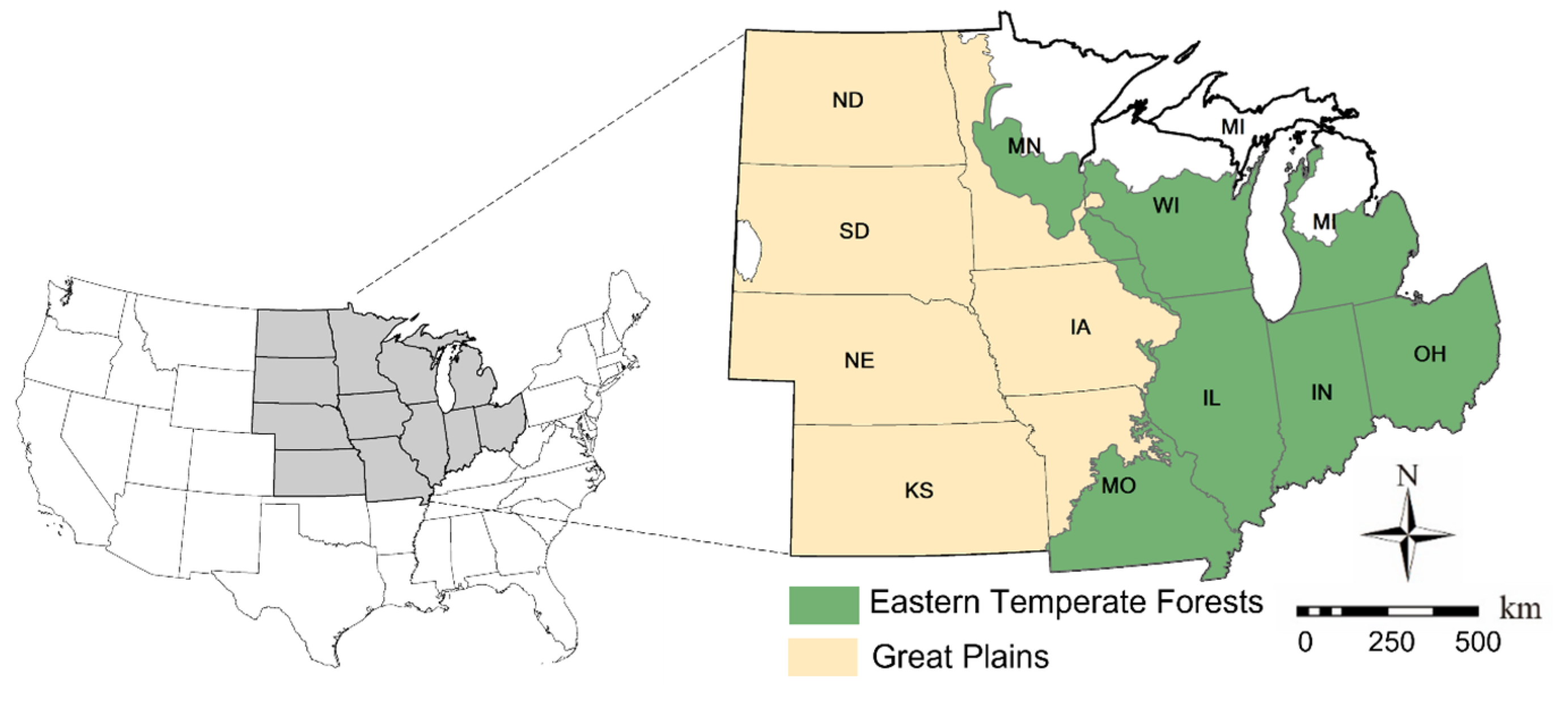
2.1. Experimental Site and Crop Yield Records

Twelve Midwestern states are included in the experimental site (Figure 1). Both corn and soybean have been grown in these states. Historical yield records of corn and soybean were downloaded from the National Agricultural Statistics Service (NASS), which is the statistical arm of the USDA and provides county-level crop yield statistics (USDA, 2020). Following previous studies [22,38], we grouped counties in the experimental sites into two distinct ecological zones. As shown in Figure 1, counties on the east side are in the Eastern Temperate Forests (ETFs) and counties on the west side are in the Great Plains (GPs). These two ecological zones are well-suited for transfer experiments due to their distinct climates and environments. Specifically, the ETFs have a humid, temperate climate with a lot of rainfall and a great level of biodiversity. The GPs, on the other hand, experience hot summers and little precipitation, resulting in a relatively low plant richness [39].

2.2. Satellite-Derived Vegetation Indices and Meteorological Variables

Three complementary VIs that have demonstrated a strong correlation with crop yields were derived from the daily MODIS MCD43A4 imagery at a spatial resolution of 500 m [15]. Specifically, the Enhanced Vegetation Index (EVI) was created based on the Normalized Difference Vegetation Index (NDVI) and has improved sensitivity in areas with abundant biomass [40]. The Green Chlorophyll Index (GCI) was designed to measure the canopy chlorophyll content, which allows it to calculate how effectively crops utilize light [41]. The Normalized Difference Water Index (NDWI) is widely used to track changes in the water content of plant leaves since it was created to measure the moisture content of vegetation [42]. The formulas of EVI, GCI, and NDWI are given below:

$$EVI=2.5\times \frac{(NIR-Red)}{NIR+C_1\times Red-C_2\times Blue+L}$$

(1)

$$GCI=\frac{NIR}{Green}-1$$

(2)

$$NDWI=\frac{NIR-SWIR}{NIR+SWIR}$$

(3)

in which the terms $Red$, $Blue$, $Green$, $NIR$, and $SWIR$ refer to the spectral bands in the red, blue, green, near-infrared, and short-wave infrared spectral channels that have been atmospherically corrected; $L$, which is set as 1 in our study, represents a constant value used for background adjustment; $C_1$ and $C_2$ are coefficients for atmospheric correction, which are set as 6.0 and 7.5, respectively [8].

In addition to VIs, meteorological variables were also considered in this study as a measurement of environmental stresses. Specifically, the land surface temperature during both daytime and nighttime was obtained from the MODIS MYD11A2 product at a spatial resolution of 1 km (i.e., LSTday and LSTnight) [43]. LSTday and LSTnight were considered because they can quantify the heat stress on the ground [9]. Meteorological variables have been extracted from the DAYMET V4 gridded daily weather dataset at a 1 km spatial resolution. Four types of meteorological variables were considered, including daily maximum air temperature (Tmax), daily minimum air temperature (Tmin), daily total precipitation (PPT), as well as incident shortwave radiation flux density (SRAD) [44]. Specifically, the air temperatures were included since they affect crop growth and development, as well as the timing of important crop stages such as flowering and maturation. PPT was considered since adequate and timely rainfall is essential for the growth and development of crops, and insufficient or excessive precipitation can have a significant impact on crop yield. Moreover, SRAD was incorporated into the feature set because of its close relationship with the photosynthesis process in plants, which is vital for crop growth and development [45].

2.3. Data Preprocessing

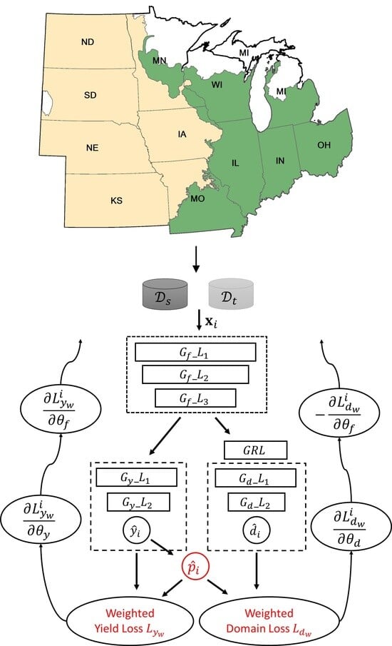
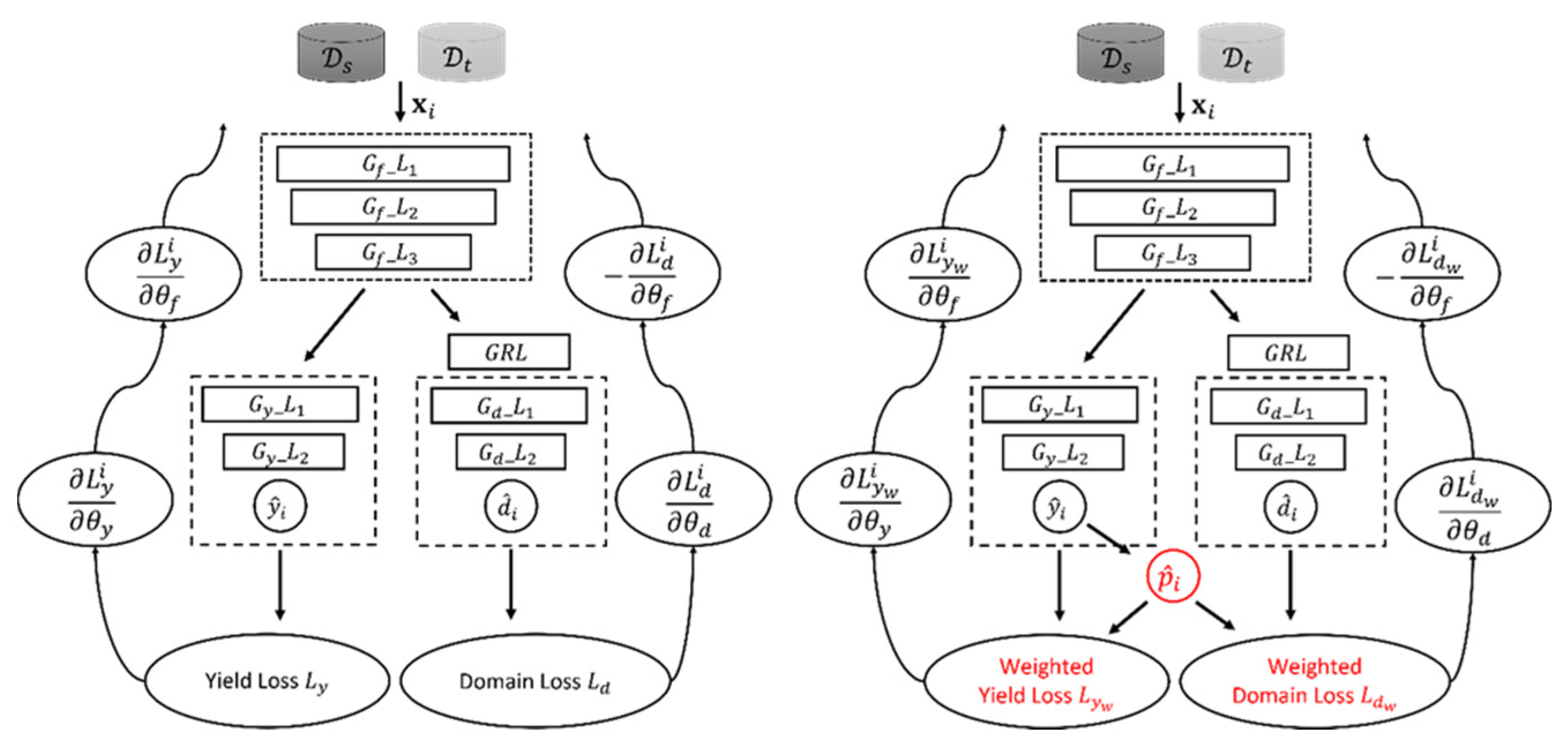
County-level crop yields, VIs, and meteorological variables were collected from 2008 to 2021. As each type of data originates from various sources and possesses diverse spatial and temporal resolutions, preprocessing becomes essential. Specifically, to eliminate noisy observations of irrelevant landcover, the Cropland Data Layer (CDL) provided by USDA-NASS was utilized as the crop mask for masking out such observations [46]. Subsequently, daily VIs and meteorological variables were initially aggregated spatially to the county level by calculating the mean value of each variable in each county using Google Earth Engine (GEE). Following this, daily VIs and meteorological variables were temporally aggregated to a 16-day interval by calculating the mean value of each time-series variable in every 16-day time window. These time-series variables were computed between March and October, covering a total of 14 periods to encompass the planting and growing season for corn and soybean in the experimental site. The resulting feature vector has a total length of 126 (i.e., 9 types of feature variables, and each has 14 periods). Finally, in each county, the yield records and the associated feature vectors were paired in the corresponding years and ready for model development.

Table 1. A summary of ecological domains and feature variables used in this study.

Domain	Environment and Climate	# Samples	Land Cover Layer	Variables
Eastern Temperate Forests (ETFs)	Largely covered by closed-canopy deciduous forests with a humid and temperate climate.	Corn: 5650 Soybean: 5658	USDA-NASS Cropland Data Layer (CDL)	EVI, NDWI, and GCI from MODIS MCD43A4 LSTday and LSTnight from MODIS MYD11A2 Tmin, Tmax, PPT, and SRAD from DAYMET
Great Plains (GPs)	Comparatively low biodiversity with a hot summer and low rainfall.	Corn: 5599 Soybean: 5229

presents a comprehensive summary of the experimental site and the feature variables utilized for model development.

3. Methodology

Supervised DL models aim to associate input features, $\mathbf{x}\in X$, with their corresponding labels, $y\in Y$, by learning the underlying probability distribution, $D\left(\mathbf{x},\mathbf{y}\right)$, that characterizes the relationship between them, in which $X$ denotes the input feature space and $Y$ denotes the label space. When predicting crop yield, $\mathbf{x}$ are feature vectors of time-series VIs and meteorological variables, and $y$ denotes the crop yield. Given the source domain dataset ${\mathcal{D}}_s$ and the target domain dataset ${\mathcal{D}}_t$, it is likely that domain shift exists between ${\mathcal{D}}_s$ and ${\mathcal{D}}_t$ due to different climates and environments. Consequently, models trained with labeled data from $D_s$ are likely to suffer from degraded performance when applied directly to $D_t$ [20].

To improve the transferability of DL models, the DANN model [47] has been proposed to address the issue of domain shift by projecting input features from each domain into a common subspace via adversarial learning. It mainly has three components: a feature extractor $G_f$, a yield predictor $G_y$, and a domain discriminator $G_d$ (Figure 2 (left)). These components are trained end-to-end, enabling the model to learn and adapt to different domains. Specifically, during the feed-forward process, the $i$th input data ${\mathbf{x}}_i$ from either ${\mathcal{D}}_s$ or ${\mathcal{D}}_t$ is initially passed through $G_f$ to extract cross-domain features ${\mathbf{x}}_i^c$ (Equation (4)). The extracted features ${\mathbf{x}}_i^c$ from ${\mathcal{D}}_s$ is further passed through $G_y$ for yield prediction and the predicted yield ${\widehat{y}}_i$ is outputted (Equation (5)). Meanwhile, the extracted features ${\mathbf{x}}_i^c$ from both domains are fed into $G_d$ for domain classification and the domain label ${\widehat{\mathbf{d}}}_i$ is outputted (Equation (6)), which identifies the domain that the input ${\mathbf{x}}_i$ originates from.

To update the network, two types of loss functions are used. The first one is the yield prediction loss $L_y$, which is defined as the mean squared error (MSE) (Equation (7)). Since we only have access to labeled samples in the source domain, $L_y$ is calculated based on the predicted yield ${\widehat{y}}_i$ and the corresponding yield label $y_i$ in the source domain for all $i\in \{\mathrm{1,2},\dots n_s$}. The second loss function is the domain loss $L_d$, which is defined as a binary cross-entropy (Equation (8)). $L_d$ is calculated by comparing the predicted domain label ${\widehat{\mathbf{d}}}_i$ with the corresponding domain label ${\mathbf{d}}_{\mathit{i}}$, which indicates the original domains of the input ${\mathbf{x}}_i$ (i.e., ${\mathbf{x}}_i~D_s\left(\mathbf{x}\right)$ if ${\mathbf{d}}_{\mathit{i}}=\left[\mathrm{1,0}\right]$; ${\mathbf{x}}_i~D_t\left(\mathbf{x}\right)$ if ${\mathbf{d}}_{\mathit{i}}=\left[\mathrm{0,1}\right]$):

$${\mathbf{x}}_i^c=G_f({\mathbf{x}}_i;{\theta }_f)),\forall i\in \{\mathrm{1,2},\dots n_s+{\mathrm{n}}_{\mathrm{t}}\}$$

(4)

$${\widehat{y}}_i=G_y({\mathbf{x}}_i^c;{\theta }_y),\forall i\in \{\mathrm{1,2},\dots n_s\}$$

(5)

$${\widehat{\mathbf{d}}}_i=G_d({\mathbf{x}}_i^c;{\theta }_d),\forall i\in \{\mathrm{1,2},\dots n_s+{\mathrm{n}}_{\mathrm{t}}\}$$

(6)

$$L_y=\frac{1}{n_s}{\sum }_{i=1}^{n_s}{\left(y_i-{\widehat{y}}_i\right)}^2$$

(7)

$$L_d=\frac{1}{n_s+n_t}{\sum }_{i=1}^{n_s+n_t}{\mathbf{d}}_i\log {\widehat{\mathbf{d}}}_i+(1-{\mathbf{d}}_i)\log (1-{\widehat{\mathbf{d}}}_i)$$

(8)

in which ${\theta }_f$, ${\theta }_y$, and ${\theta }_d$ denote the trainable weights in $G_f$, $G_y$, and $G_d$, respectively. $n_s$ denotes the number of labeled data samples in the source domain and $n_t$ denotes the number of unlabeled data samples in the target domain.

During backpropagation, in order to extract features ${\mathbf{x}}_i^c$ that are informative to the main task (i.e., accurately predict crop yield) and indiscriminative between domains (i.e., have small domain shift), the feature extractor $G_f$ is trained in collaboration with the yield predictor $G_y$ to minimize $L_y$. Additionally, it is trained adversarially with the domain discriminator $G_d$ to maximize $L_d$. To perform adversarial training between $G_f$ and $G_d$, the gradient reversal layer (GRL) is inserted to connect $G_f$ and $G_d$, which reverses the direction of the gradient during backpropagations. Overall, the loss function combining the yield prediction loss and the domain loss is given by (Equation (9)):

$$L=L_y-\lambda L_d$$

(9)

where $\lambda$ is a weighting parameter that determines the balance between two losses. Though successful, the DANN model is trained to match the target domain with the whole source domain under the assumption that they share an identical label space (i.e., $Y_s=Y_t)$. Unfortunately, it may not hold true in the context of large-scale crop yield prediction, as yield distributions tend to vary across different regions. Therefore, the DANN could mistakenly align source samples and target samples with very different yields and result in negative transfer.

To address the aforementioned issue, an intuitive solution is to reduce the contribution of those source samples assigned to the outlier label space $Y_s\backslash Y_t$, which refers to a subset of the source domain that has labels not appearing in the target domain. However, determining if a source sample falls within the outlier label space $Y_s\backslash Y_t$ can be a challenging task owning to the fact that historical yield records are not available in the target domain. Fortunately, using the predicted yield ${\widehat{y}}_i$ for target inputs provided by the yield predictor, we can estimate the target yield distribution. The estimated target yield distribution can be used to assess the likelihood of a source sample falling into the outlier label space. Given that $Y_s\backslash Y_t$ and $Y_t$ are disjointed, the feature distributions in the outlier source label space ought to differ from the feature distributions of target samples. Consequently, the estimated target yield distribution should have a low probability of such outlier samples from the source domain. In contrast, feature distributions of the source samples within the shared label space $Y_s\cup Y_t$ should resemble those of the target samples more closely. Therefore, the corresponding yield values of source samples within $Y_s\cup Y_t$ should have a high probability given the estimated target yield distribution.

Based on this idea, we proposed the partial DANN (PDANN) model, which downweighs source samples in the outlier label space according to the estimated yield distribution in the target domain. As depicted in Figure 2 (right), the proposed PDANN has a similar architecture to the DANN model but has a different training procedure. Specifically, the PDANN model is first pre-trained as a DANN model for a few epochs to establish an initial association between $\mathbf{x}$ and $y$. After that, input data ${\mathbf{x}}_i$ from either ${\mathcal{D}}_s$ or ${\mathcal{D}}_t$ are passed through the feature extractor $G_f$ to extract cross-domain features. The extracted feature ${\mathbf{x}}_i^c$ from both domains is further passed through the yield predictor $G_y$ to predict the crop yield ${\widehat{y}}_i$. Meanwhile, ${\mathbf{x}}_i^c$ is also forwarded into the domain discriminator $G_d$ for domain classification and outputs the domain label ${\widehat{\mathbf{d}}}_i$. These predicted yields for the target samples from ${\mathcal{D}}_t$ are used to estimate the yield distribution as a normal distribution $N({\widehat{\mu }}_t,{\widehat{\sigma }}_t)$ (Equations (10) and (11)). The normal distribution is adapted here since it is a common assumption in regression when a large number of data samples are available. After that, the PDANN estimates the weight for each crop yield record $y_i$ from ${\mathcal{D}}_s$ according to its likelihood ${\widehat{p}}_i$ given $N({\widehat{\mu }}_t,{\widehat{\sigma }}_t)$ (Equation (12)). A higher ${\widehat{p}}_i$ indicates that the source sample is more likely to be within the common label space while a lower ${\widehat{p}}_i$ indicates that it is more likely to be in the outlier label space. With ${\widehat{p}}_i$, PDANN can reduce the contribution of source samples in the outlier label space $Y_s\backslash Y_t$. As such, each source sample is weighted according to ${\widehat{p}}_i$ and the weighted yield prediction loss $L_{y_w}$ (Equation (13)) and weighted domain loss $L_{d_w}$ (Equation (14)) are calculated as below:

$${\widehat{\mu }}_t=\frac{1}{n_t}{\sum }_{i=1}^{n_t}{\widehat{y}}_i$$

(10)

$${\widehat{\sigma }}_t=\sqrt{\frac{{\left({\widehat{y}}_i-{\widehat{\mu }}_t\right)}^2}{n_t-1}}$$

(11)

$${\widehat{p}}_i(y_i)=\frac{1}{\sqrt{2\pi }{\widehat{\sigma }}_t}\exp (\frac{{\left({\widehat{\mu }}_t-y_i\right)}^2}{2{\widehat{\sigma }}_t^2})$$

(12)

$$L_{y_w}=\frac{1}{n_s}{\sum }_{i=1}^{n_s}{\widehat{p}}_i\left(y_i\right){\left(y_i-{\widehat{y}}_i\right)}^2$$

(13)

$$\begin{array}{cc}\hfill L_{d_w}=& \frac{1}{n_s}{\sum }_{i=1}^{n_s}{\widehat{p}}_i\left(y_i\right)({\mathbf{d}}_i\log {\widehat{\mathbf{d}}}_i+(1-{\mathbf{d}}_i\left)\log (1-{\widehat{\mathbf{d}}}_i)\right)\hfill \\ & +\frac{1}{n_t}{\sum }_{i=1}^{n_t}({\mathbf{d}}_i\log {\widehat{\mathbf{d}}}_i+(1-{\mathbf{d}}_i\left)\log (1-{\widehat{\mathbf{d}}}_i)\right)\hfill \end{array}$$

(14)

in which ${\widehat{\mu }}_t$ and ${\widehat{\sigma }}_t$ denote the estimated mean and standard deviation for the estimated yield distribution in the target domain. ${\widehat{p}}_i\left(y_i\right)$ is the likelihood of the ground truth yield records $y_i$ given the estimated target yield distribution $N({\widehat{\mu }}_t,{\widehat{\sigma }}_t)$. Note that the weighted yield prediction loss $L_{y_w}$ is calculated based on the labeled source samples since ground truth label information in the target domain is not available during training.

Our proposed PDANN has been designed with a depth of six. In particular, $G_f$ has an input layer and three hidden layers comprising 256, 128, and 64 neurons. Neighboring hidden layers are fully connected with each other. Meanwhile, both $G_d$ and $G_y$ are made up of two hidden layers, with 64 and 32 neurons, respectively, and an output layer. Like the feature extractor, the neighboring hidden layers and the output layer are fully connected in $G_d$ and $G_y$. The activation function for each hidden neuron was the Rectified Linear Unit (ReLU). Similar to DANN, the GRL is employed to link the feature extractor and the domain classifier, facilitating the reversal of gradient signs during backpropagation. Based on our experiments, the maximum training epochs was set as 200 and the PDANN model was pre-trained in the first 20 epochs. The Adam optimization algorithm was used as the optimizer [48].

4. Experiments and Results

4.1. Experiment Setup

We evaluated the proposed PDANN model in predicting the yield of the two main commodities in the U.S., namely corn and soybean. Besides PDANN, three other approaches were selected as comparison methods. The first comparison model is the random forest (RF), which is one of the most widely used ML-based yield prediction methods [9,49,50,51]. We implemented the RF model in Python using the scikit-learn library, a widely-used ML toolkit that provides efficient and user-friendly implementations of various algorithms [52]. The second model for comparison is the deep neural network with fully connected layers (DNN), which is a representative model in the field of deep learning [25]. The third model for comparison is the ADANN model, which is a DANN-based UDA model for regression tasks such as crop yield prediction [31] and robot deformation prediction [32]. The architecture of the DNN and ADANN is identical to that of PDANN. However, the DNN does not have the domain discriminator and the ADANN does not utilize the weighting mechanism. We developed all of the DL models using PyTorch, a Python-based DL framework [53]. To train and test these models, we utilized Google Colab, a cloud-based platform for ML, which provided access to GPUs for faster processing.

Our PDANN model, along with three comparison models, underwent evaluation in two transfer experiments, where the source and target domains were alternatively defined as GP and ETF (i.e., GP → ETF and ETF → GP). Both the supervised learning models, RF and DNN, were trained using labeled source data and directly used to make yield prediction and evaluated in the target domain. The UDA methods, ADANN and PDANN, were trained with labeled source samples and unlabeled target samples. Each model was trained using data from all preceding years, since 2008, and evaluated on three testing years: 2019, 2020, and 2021. In each testing year, the R² and the RMSE (Equations (15) and (16)) were utilized to evaluate the model performance:

$${\mathrm{R}}^2=1-\frac{{\sum }_{i=1}^n{\left({\widehat{y}}_i-y_i\right)}^2}{{\sum }_{i=1}^n{\left(\overline{y}-y_i\right)}^2}$$

(15)

$$\mathrm{R}\mathrm{M}\mathrm{S}\mathrm{E}=\sqrt{\frac{1}{n}{\sum }_{i=1}^n{\left(y_i-{\widehat{y}}_i\right)}^2}$$

(16)

where ${\widehat{y}}_i$ is the predicted yield by models and $y_i$ is the corresponding reported yield; $\overline{y}$ is the average yield of all data samples; and $n$ denotes the total number of samples in a given testing year.

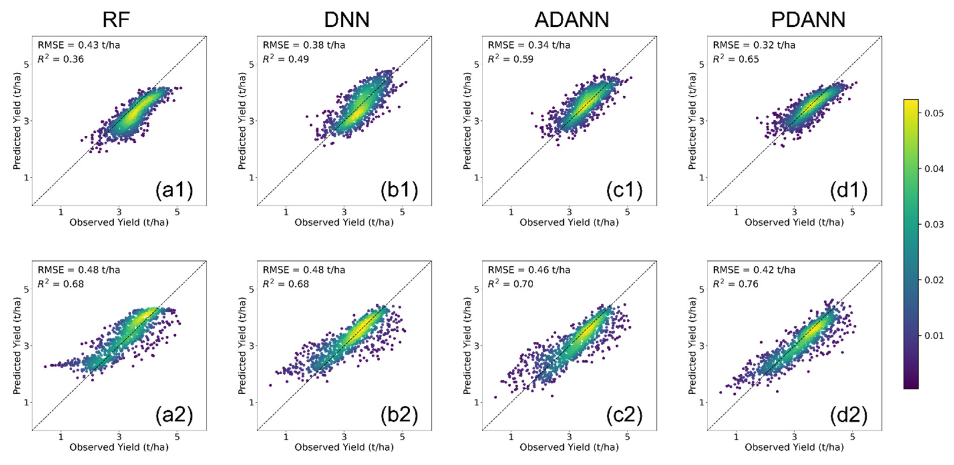
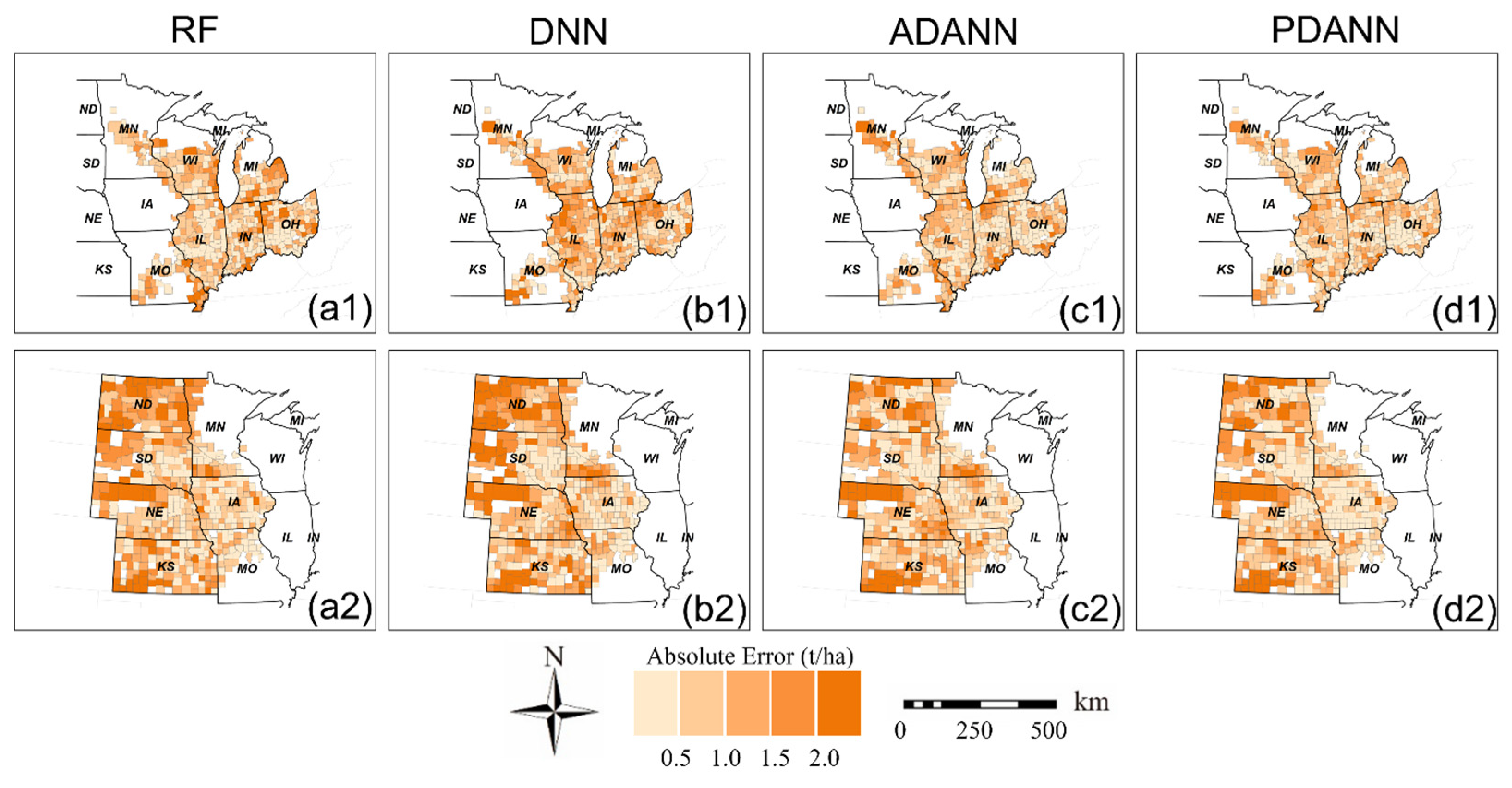
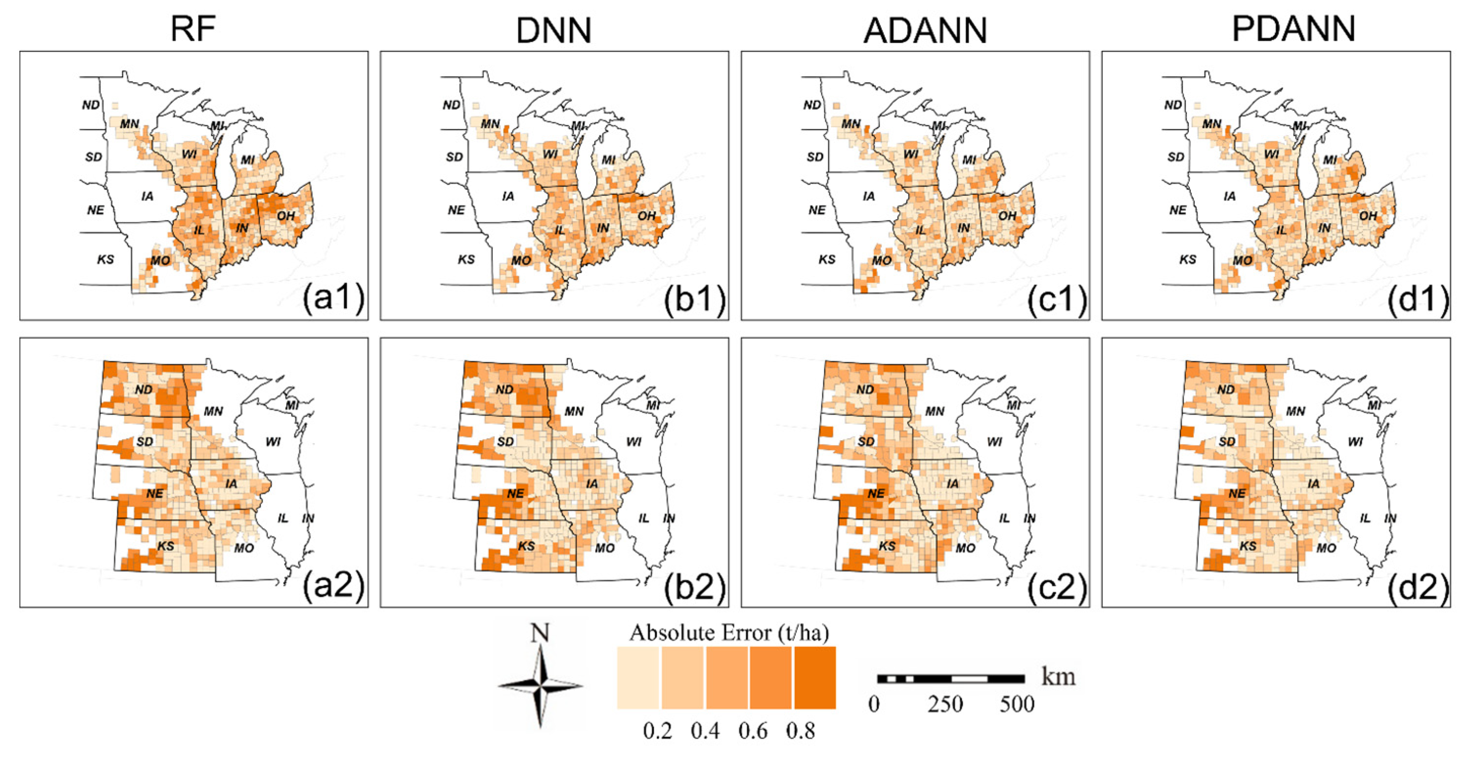
4.2. Evaluation Results

In

Table 2. Evaluation results of R² and RMSE (t/ha) for corn yield prediction in 2019–2021. The best performance is highlighted in bold.

Year	Experiment	RF		DNN		ADANN		PDANN
		R2	RMSE	R2	RMSE	R2	RMSE	R2	RMSE
2019	GP → ETF	0.33	1.13	0.37	1.09	0.53	0.94	0.56	0.91
	ETF → GP	0.70	1.28	0.68	1.31	0.73	1.20	0.78	1.10
2020	GP → ETF	0.52	1.06	0.59	1.28	0.67	0.89	0.71	0.83
	ETF → GP	0.54	1.67	0.64	1.46	0.75	1.22	0.77	1.18
2021	GP → ETF	0.53	1.08	0.49	1.17	0.59	1.01	0.65	0.94
	ETF → GP	0.75	1.67	0.71	1.80	0.74	1.70	0.75	1.67

and

Table 3. Evaluation results of R² and RMSE (t/ha) for soybean yield prediction in 2019–2021. The best performance is highlighted in bold.

Year	Experiment	RF		DNN		ADANN		PDANN
		R2	RMSE	R2	RMSE	R2	RMSE	R2	RMSE
2019	GP → ETF	0.01	0.46	0.31	0.39	0.50	0.33	0.53	0.31
	ETF → GP	0.69	0.35	0.65	0.39	0.74	0.34	0.74	0.34
2020	GP → ETF	0.27	0.20	0.50	0.33	0.56	0.31	0.65	0.28
	ETF → GP	0.67	0.44	0.62	0.47	0.68	0.43	0.72	0.40
2021	GP → ETF	0.42	0.42	0.53	0.39	0.56	0.37	0.60	0.35
	ETF → GP	0.75	0.53	0.64	0.64	0.74	0.54	0.79	0.49

, we present the evaluation results for corn and soybean yield prediction, respectively, for each testing year. Each experiment was repeated five times and the average R² and RMSE were reported for each case. The result with the highest evaluation accuracy for each case is highlighted in bold.

As observed from Table 2 and Table 3, experiments ETF → GP for both corn and soybean yield predictions consistently show substantially higher agreement R² than those of the experiments GP → ETF for each test model for test years 2020 and 2021. Contrarily, the RMSEs of experiments ETF → GP for both crops are significantly higher than those of the experiments GP → ETF for each model for 2020 and 2021. However, in 2019, the experiments GP → ETF for both corn yield predictions show comparatively lower R² than the other years. Similarly, the RMSE of the RF model for soybean yield prediction in the experiment ETF → GP is smaller than that of the experiment GP → ETF while the RMSEs of the other models for experiment ETF → GP are very close or slightly bigger than those of the GP → ETF. It is because record-breaking rainfall in 2019 caused flooding and historic delays in the pace of U.S. corn and soybean planting, especially in Illinois. As a result, it is hard to achieve high prediction agreement in experiments GP → ETF in 2019 for all models.

Specifically, due to domain shift between ETF and GP, the supervised learning models RF and DNN, which were trained solely with labeled source samples, generally underperformed in most cases. In transfer experiments from GP to ETF for corn yield prediction, both the RF and DNN made predictions that had a low agreement with the ground truth data and had an R² less than 0.60 (Table 2), especially in the abnormal year 2019. In experiments ETF → GP, the RF and DNN achieved comparatively higher R² but also had higher RMSEs for 2020 and 2021. Specifically, in experiments ETF → GP in 2020 and 2021 (Table 2), the RF had a high RMSE of 1.67 t/ha in both years. Similarly, when predicting soybean yield, the RF and DNN had low accuracy in most cases (Table 3). For example, in the experiment GP → ETF in 2019, the RF achieved an R² as low as 0.01 while the DNN also had a low R² of 0.31 (Table 3).

Both the ADANN and PDANN models employed the UDA strategy of adversarial learning to project the input features into a cross-domain subspace, thereby reducing domain shift. Consequently, the predicted yields by the ADANN and PDANN have achieved higher agreement with the reported yield (Table 2 and Table 3). Specifically, the ADANN model outperformed the supervised learning models in most cases. For example, in the year 2019, the ADANN outperformed the DNN by large margins and improved the R² from 0.33 to 0.53 in predicting corn yields (Table 2) and improved the R² from 0.31 to 0.50 in predicting soybean yields (Table 3) in the experiment GP → ETF. However, its improvements were not obvious in some cases. For example, in the experiment ETF → GP for soybean yield prediction, the ADANN model slightly improved the R² by 0.01 compared to the RF in 2020. The proposed PDANN model further outperformed the ADANN model and had more stable performance. Specifically, the PDANN model mostly improved the R² by 0.02–0.04 for both corn and soybean yield prediction in comparison with the ADANN. For soybean yield prediction from the GPs to the ETFs in 2020, the PDANN largely improved the R² by 0.09 in comparison with the ADANN (Table 3). It proved that the PDANN was more effective in addressing the domain shift, providing greater robustness than other methods.

In order to visually demonstrate the level of agreement between reported and predicted yields, we present the density scatter plots in Figure 3 and Figure 4. In all cases, the proposed PDANN model demonstrated the highest level of agreement (Figure 3(d1,d2) and Figure 4(d1,d2)). Specifically, owing to the domain shift between ETFs and GPs, predictions by RF and DNN tend to be biased. However, such biases are not consistent between low yield counties and high yield counties. For example, since the crop yields are comparatively lower in the GP, the RF and DNN were observed to underestimate the crop yields in ETF when trained with labeled data in GP for both corn and soybean. On the other hand, as shown in Figure 3(a2,b2) and Figure 4(a2), the ETF → GP yields were overestimated for the RF and DNN. Similarly, as shown in Figure 4(b2), the low yield counties (less than 10 tons/ha for corn and less than 3 tons/ha for soybeans), were overestimated for ETF → GP while the high yield counties were underestimated. After UDA, both the ADANN and the PDANN reduced the bias and achieved better agreement. Moreover, the scatter plots of the PDANN were more compact and less variant than the ADANN model’s, suggesting its superior performance.

Finally, we present in Figure 5 and Figure 6 the average absolute error maps from 2019 to 2021 for corn and soybean yield prediction, respectively, with darker colors indicating larger absolute error values for each model. The results showed that RF and DNN models exhibited smaller errors in states near the boundary of ETF and GP, such as IL (Figure 5(a1) and Figure 6(b1)), while a cluster of large errors was observed in states distant from the other domain, such as OH, IN, ND, SD, and western NE. This is because the domain shift would be more significant in areas located away from the source domain. Compared to the RF and DNN, the ADANN model eliminated most error clusters and reduced absolute errors in ND, SD, and IN (Figure 5(c1,c2) and Figure 6(c1,c2)). The PDANN further improved the prediction accuracy compared to the ADANN. It had smaller errors in most counties, especially in IA for corn yield prediction (Figure 5(d2)) and in NE and KS for soybean yield prediction (Figure 6(d2)).

5. Discussion

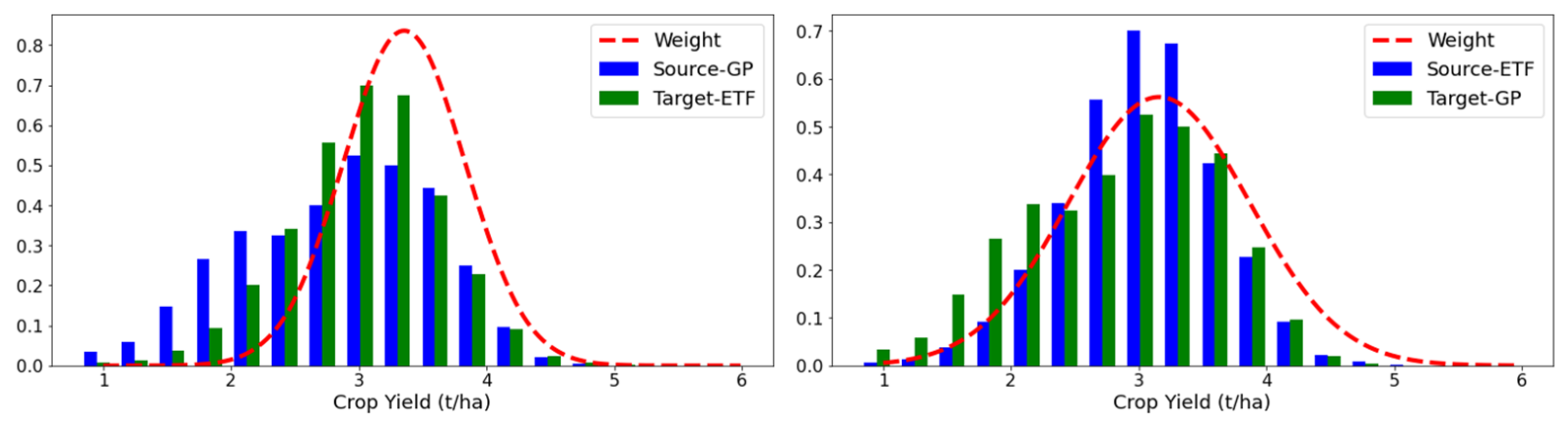
5.1. Weighting Mechanism Analysis

To explore the weighting mechanism in the proposed PDANN, we depicted the calculated weights for the PDANN together with the yield distributions in each domain (Figure 7 and Figure 8). Given that consistent results were obtained over multiple years, we have presented the results in 2021 as a representative example.

It was observed that the yield distributions of both corn and soybean in the ETFs and GPs were significantly different, indicating that their label spaces were not identical. In the transfer experiments of corn yield prediction, when transferring from the GPs to the ETFs (Figure 7 (left)), a large portion of counties in the GPs had a low corn yield, below 8.00 t/ha, while only a few counties in the ETFs had similar yields. Despite a lack of yield records in the target domain, the PDANN successfully captured the difference between the label spaces and downweighed source samples with low yields in the GPs. When transferring from the ETFs to the GPs, most of the labeled samples from the ETFs were in the range of 10.00~12.00 t/ha while very few of them were in the range of 6.00~8.00 t/ha. Instead of matching the target domain to the whole source domain, the PDANN model performed partial domain adaptation by proportionally assigning weights to data samples with different yields (Figure 7 (right)).

Similarly, in the experiments of soybean yield prediction, when transferring from the GPs to ETFs (Figure 8 (left)), a large portion of counties in the GPs had a yield below 2.00 t/ha, while only a few counties in the ETFs had such low yields. Again, the PDANN captured the difference between the label spaces and downweighed source samples with low yields in the GPs. When transferring from the ETFs to the GPs, most of the labeled samples from the ETFs exhibited a yield of around 3.00 t/ha, with only a small number of counties having a yield of less than 2.00 t/ha. Correspondingly, the PDANN assigned large weights to source data samples in the ETFs that had a yield of around 2.00~3.00 t/ha to promote positive transfer by aligning the feature distributions of data samples within the shared label space (Figure 8 (right)).

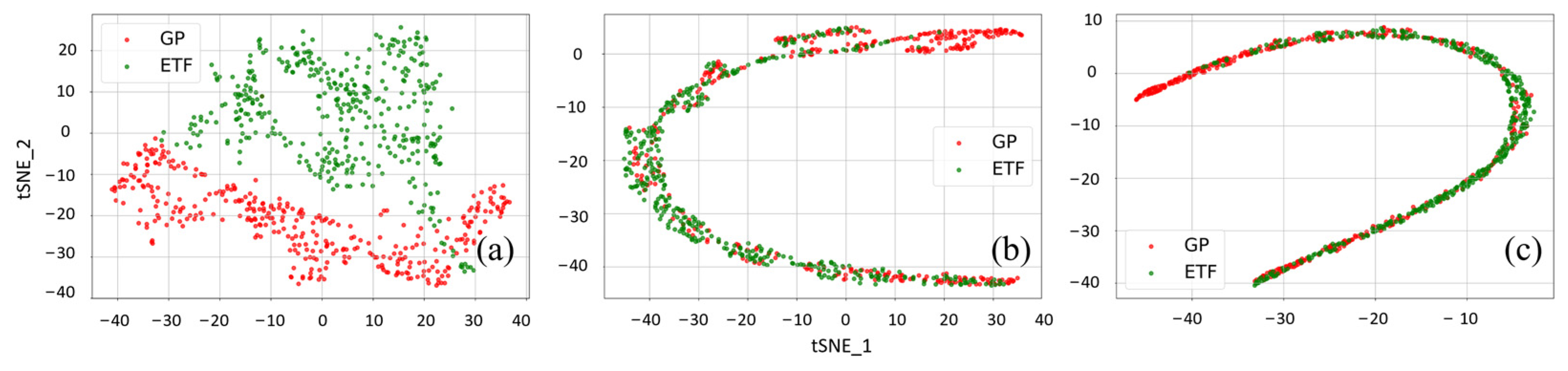
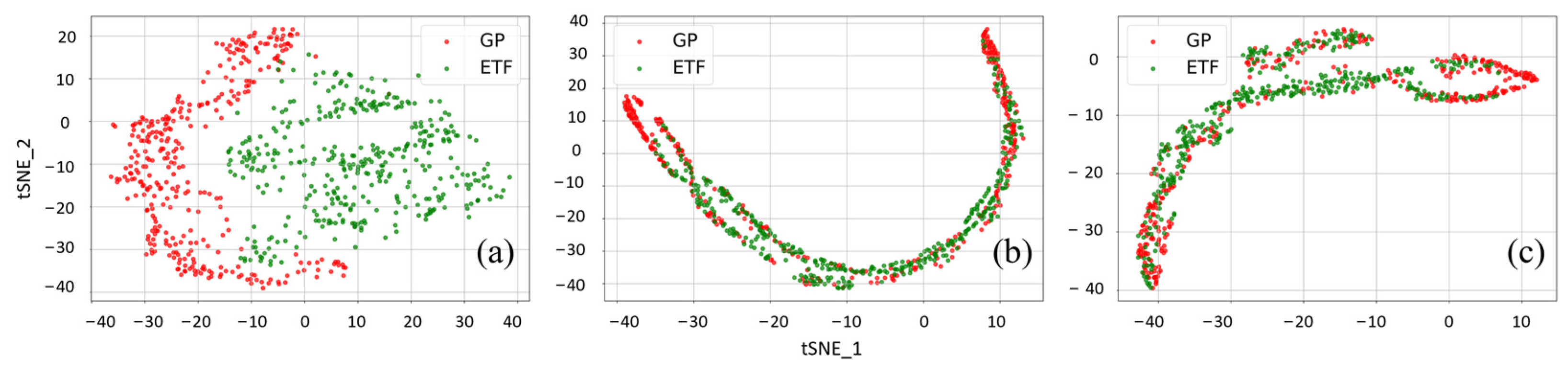
5.2. t-SNE Visualization

We also utilized t-distributed Stochastic Embedding (t-SNE) to visualize the distributions of both the input features and cross-domain features extracted by the PDANN, in which high-dimensional feature vectors were projected onto a two-dimensional space [54].

As shown in Figure 9 and Figure 10, we present the t-SNE visualization of the original input features and cross-domain features extracted by the PDANN in the transfer experiments in 2021. The original input features were mapped from the original feature space with a length of 126 to the 2D space (Figure 9 and Figure 10a). Similarly, the extracted features were mapped from the subspace with a length of 64 to the 2D space (Figure 9 and Figure 10b,c). Data samples from the GPs and ETFs are color-coded by green and red, accordingly. Similar samples are supposed to be close while dissimilar samples are distant.

Before UDA, it was observed that the original input features from the GPs and ETFs had very different distributions with small overlapping areas, which indicates that significant domain shifts exist between these two domains (Figure 9 and Figure 10a). After UDA, PDANN successfully reduced domain shifts and extracted features with similar distributions (Figure 9 and Figure 10b,c). Additionally, it was notable that some source samples were not matched with data samples from the target domain (Figure 9 and Figure 10). Such data samples could be in the outlier label space and the PDANN model did not force them to be aligned with the target domain by applying very low weights. It demonstrated that the weighting mechanism enabled the PDANN model to effectively minimize the misalignment between target samples and outlier source samples.

6. Conclusions

ML and DL models have been increasingly used for crop yield prediction but are facing issues of low transferability due to domain shifts between different spatial regions. Recently, UDA has emerged as a promising approach for improving the transferability of DL models. However, UDA methods may be susceptible to negative transfer due to label space mismatches, such as significant variations in yield distributions across different regions. To tackle this issue, an effective strategy is to diminish the impact of source samples in the outlier label space and partially align source and target domains in the shared label space, which is referred to as a PDA. In this study, we adapted this strategy and proposed a PDANN model via adversarial learning for county-level crop yield prediction based on satellite-derived VIs and meteorological variables. Rather than matching the target domain with the whole source domain, the PDANN downweighed the source samples in the outlier label space during model training through an innovative weighting mechanism. Transfer experiments between two distinct ecological zones in the Midwest of the U.S. demonstrated that a PDANN further improved yield prediction accuracies for both corn and soybean. The PDANN model outperformed commonly used supervised learning models (i.e., RF and DNN) and adversarial domain adaptation models (i.e., ADANN) in three testing years 2019–2021. Model interpretation showed that the weighting mechanism enabled the PDANN model to avoid negative transfer by reducing the contribution of outlier source samples and promoting positive transfer by aligning the feature distributions in the shared label space. Although this study has successfully demonstrated the effectiveness of PDA for predicting crop yields, there are still several avenues for future research. One potential direction is to explore the effectiveness of PDA on field-level yield mapping. Another area for future research is to investigate how the PDANN model can be integrated with farm management systems to improve yield monitoring, which could have significant practical implications for agriculture.

References

1. Kluger, D.M.; Owen, A.B.; Lobell, D.B. Combining randomized field experiments with observational satellite data to assess the benefits of crop rotations on yields. Environ. Res. Lett. 2022, 17, 044066. [Google Scholar] [CrossRef]
2. Dado, W.T.; Deines, J.M.; Patel, R.; Liang, S.-Z.; Lobell, D.B. High-Resolution Soybean Yield Mapping Across the US Midwest Using Subfield Harvester Data. Remote Sens. 2020, 12, 3471. [Google Scholar] [CrossRef]
3. Gao, F.; Anderson, M.; Daughtry, C.; Johnson, D. Assessing the Variability of Corn and Soybean Yields in Central Iowa Using High Spatiotemporal Resolution Multi-Satellite Imagery. Remote Sens. 2018, 10, 1489. [Google Scholar] [CrossRef]
4. Lobell, D.B.; Hammer, G.L.; McLean, G.; Messina, C.; Roberts, M.J.; Schlenker, W. The critical role of extreme heat for maize production in the United States. Nat. Clim. Chang. 2013, 3, 497–501. [Google Scholar] [CrossRef]
5. Zhou, W.; Guan, K.; Peng, B.; Tang, J.; Jin, Z.; Jiang, C.; Grant, R.; Mezbahuddin, S. Quantifying carbon budget, crop yields and their responses to environmental variability using the ecosys model for U.S. Midwestern agroecosystems. Agric. For. Meteorol. 2021, 307, 108521. [Google Scholar] [CrossRef]
6. Lv, Z.; Huang, H.; Li, X.; Zhao, M.; Benediktsson, J.A.; Sun, W.; Falco, N. Land Cover Change Detection with Heterogeneous Remote Sensing Images: Review, Progress, and Perspective. Proc. IEEE 2022, 110, 1976–1991. [Google Scholar] [CrossRef]
7. Wang, Y.; Zhang, Z.; Feng, L.; Ma, Y.; Du, Q. A new attention-based CNN approach for crop mapping using time series Sentinel-2 images. Comput. Electron. Agric. 2021, 184, 106090. [Google Scholar] [CrossRef]
8. Kang, Y.; Ozdogan, M.; Zhu, X.; Ye, Z.; Hain, C.R.; Anderson, M.C. Comparative assessment of environmental variables and machine learning algorithms for maize yield prediction in the US Midwest. Environ. Res. Lett. 2020, 15, 064005. [Google Scholar] [CrossRef]
9. Johnson, D.M. An assessment of pre- and within-season remotely sensed variables for forecasting corn and soybean yields in the United States. Remote Sens. Environ. 2014, 141, 116–128. [Google Scholar] [CrossRef]
10. Kamir, E.; Waldner, F.; Hochman, Z. Estimating wheat yields in Australia using climate records, satellite image time series and machine learning methods. ISPRS J. Photogramm. Remote Sens. 2019, 160, 124–135. [Google Scholar] [CrossRef]
11. Marshall, M.; Belgiu, M.; Boschetti, M.; Pepe, M.; Stein, A.; Nelson, A. Field-level crop yield estimation with PRISMA and Sentinel-2. ISPRS J. Photogramm. Remote Sens. 2022, 187, 191–210. [Google Scholar] [CrossRef]
12. Chen, S.; Liu, W.; Feng, P.; Ye, T.; Ma, Y.; Zhang, Z. Improving Spatial Disaggregation of Crop Yield by Incorporating Machine Learning with Multisource Data: A Case Study of Chinese Maize Yield. Remote Sens. 2022, 14, 2340. [Google Scholar] [CrossRef]
13. Sun, J.; Di, L.; Sun, Z.; Shen, Y.; Lai, Z. County-Level Soybean Yield Prediction Using Deep CNN-LSTM Model. Sensors 2019, 19, 4363. [Google Scholar] [CrossRef]
14. Zhang, L.; Zhang, Z.; Luo, Y.; Cao, J.; Xie, R.; Li, S. Integrating satellite-derived climatic and vegetation indices to predict smallholder maize yield using deep learning. Agric. For. Meteorol. 2021, 311, 108666. [Google Scholar] [CrossRef]
15. Ma, Y.; Zhang, Z.; Kang, Y.; Özdoğan, M. Corn yield prediction and uncertainty analysis based on remotely sensed variables using a Bayesian neural network approach. Remote Sens. Environ. 2021, 259, 112408. [Google Scholar] [CrossRef]
16. Hunt, M.L.; Blackburn, G.A.; Carrasco, L.; Redhead, J.W.; Rowland, C.S. High resolution wheat yield mapping using Sentinel-2. Remote Sens. Environ. 2019, 233, 111410. [Google Scholar] [CrossRef]
17. Nguyen, L.H.; Robinson, S.; Galpern, P. Medium-resolution multispectral satellite imagery in precision agriculture: Mapping precision canola (Brassica napus L.) yield using Sentinel-2 time series. Precis. Agric. 2022, 23, 1051–1071. [Google Scholar] [CrossRef]
18. Lv, Z.; Zhang, P.; Sun, W.; Benediktsson, J.A.; Li, J.; Wang, W. Novel Adaptive Region Spectral–Spatial Features for Land Cover Classification With High Spatial Resolution Remotely Sensed Imagery. IEEE Trans. Geosci. Remote Sens. 2023, 61, 5609412. [Google Scholar] [CrossRef]
19. Wang, Y.; Zhang, Z.; Feng, L.; Du, Q.; Runge, T. Combining Multi-Source Data and Machine Learning Approaches to Predict Winter Wheat Yield in the Conterminous United States. Remote Sens. 2020, 12, 1232. [Google Scholar] [CrossRef]
20. Kouw, W.M.; Loog, M. An Introduction to Domain Adaptation and Transfer Learning. 2018. Available online: http://arxiv.org/abs/1812.11806 (accessed on 15 September 2023).
21. Tuia, D.; Persello, C.; Bruzzone, L. Domain Adaptation for the Classification of Remote Sensing Data: An Overview of Recent Advances. IEEE Geosci. Remote Sens. Mag. 2016, 4, 41–57. [Google Scholar] [CrossRef]
22. Ma, Y.; Zhang, Z. A Bayesian Domain Adversarial Neural Network for Corn Yield Prediction. IEEE Geosci. Remote Sens. Lett. 2022, 19, 5513705. [Google Scholar] [CrossRef]
23. Chew, R.; Rineer, J.; Beach, R.; O’neil, M.; Ujeneza, N.; Lapidus, D.; Miano, T.; Hegarty-Craver, M.; Polly, J.; Temple, D.S. Deep Neural Networks and Transfer Learning for Food Crop Identification in UAV Images. Drones 2020, 4, 7. [Google Scholar] [CrossRef]
24. Wang, A.X.; Tran, C.; Desai, N.; Lobell, D.; Ermon, S. Deep Transfer Learning for Crop Yield Prediction with Remote Sensing Data. In Proceedings of the 1st ACM SIGCAS Conference on Computing and Sustainable Societies, San Jose, CA, USA, 20–22 June 2018. [Google Scholar] [CrossRef]
25. Khaki, S.; Pham, H.; Wang, L. Simultaneous corn and soybean yield prediction from remote sensing data using deep transfer learning. Sci. Rep. 2021, 11, 11132. [Google Scholar] [CrossRef] [PubMed]
26. Zhao, Y.; Han, S.; Meng, Y.; Feng, H.; Li, Z.; Chen, J.; Song, X.; Zhu, Y.; Yang, G. Transfer-Learning-Based Approach for Yield Prediction of Winter Wheat from Planet Data and SAFY Model. Remote Sens. 2022, 14, 5474. [Google Scholar] [CrossRef]
27. Schwalbert, R.A.; Amado, T.; Corassa, G.; Pott, L.P.; Prasad, P.; Ciampitti, I.A. Satellite-based soybean yield forecast: Integrating machine learning and weather data for improving crop yield prediction in southern Brazil. Agric. For. Meteorol. 2020, 284, 107886. [Google Scholar] [CrossRef]
28. Zhao, S.; Yue, X.; Zhang, S.; Li, B.; Zhao, H.; Wu, B.; Krishna, R.; Gonzalez, J.E.; Sangiovanni-Vincentelli, A.L.; Seshia, S.A.; et al. A Review of Single-Source Deep Unsupervised Visual Domain Adaptation. IEEE Trans. Neural Netw. Learn. Syst. 2020, 33, 473–493. [Google Scholar] [CrossRef] [PubMed]
29. Wang, Q.; Rao, W.; Sun, S.; Xie, L.; Chng, E.S.; Li, H. Unsupervised Domain Adaptation via Domain Adversarial Training for Speaker Recognition. ICASSP IEEE Int. Conf. Acoust. Speech Signal Process. Proc. 2018, 2018, 4889–4893. [Google Scholar] [CrossRef]
30. Han, T.; Liu, C.; Yang, W.; Jiang, D. A novel adversarial learning framework in deep convolutional neural network for intelligent diagnosis of mechanical faults. Knowl.-Based Syst. 2019, 165, 474–487. [Google Scholar] [CrossRef]
31. Ma, Y.; Zhang, Z.; Yang, H.L.; Yang, Z. An adaptive adversarial domain adaptation approach for corn yield prediction. Comput. Electron. Agric. 2021, 187, 106314. [Google Scholar] [CrossRef]
32. Ye, C.; Yang, J.; Ding, H. High-accuracy prediction and compensation of industrial robot stiffness deformation. Int. J. Mech. Sci. 2022, 233, 107638. [Google Scholar] [CrossRef]
33. Ma, Y.; Yang, Z.; Zhang, Z. Multi-source Maximum Predictor Discrepancy for Unsupervised Domain Adaptation on Corn Yield Prediction. IEEE Trans. Geosci. Remote Sens. 2023, 61, 4401315. [Google Scholar] [CrossRef]
34. Gu, X.; Yu, X.; Yang, Y.; Sun, J.; Xu, Z. Adversarial Reweighting for Partial Domain Adaptation. Adv. Neural Inf. Process. Syst. 2021, 18, 14860–14872. [Google Scholar]
35. Zhang, J.; Ding, Z.; Li, W.; Ogunbona, P. Importance Weighted Adversarial Nets for Partial Domain Adaptation. In Proceedings of the 2018 IEEE/CVF Conference on Computer Vision and Pattern Recognition, Salt Lake City, UT, USA, 18–23 June 2018; pp. 8156–8164. [Google Scholar] [CrossRef]
36. Cao, Z.; Ma, L.; Long, M.; Wang, J. Partial Adversarial Domain Adaptation. In Proceedings of the European Conference on Computer Vision (ECCV), Munich, Germany, 8–14 September 2018; 11212, pp. 139–155. [Google Scholar] [CrossRef]
37. Cao, Z.; Long, M.; Wang, J.; Jordan, M.I. Partial Transfer Learning with Selective Adversarial Networks. In Proceedings of the 2018 IEEE/CVF Conference on Computer Vision and Pattern Recognition, Salt Lake City, UT, USA, 18–23 June 2018; pp. 2724–2732. [Google Scholar] [CrossRef]
38. Russello, H. Convolutional Neural Networks for Crop Yield Prediction using Satellite Images. M.S. Thesis. IBM Cent. Adv. Stud.. 2018. Available online: https://www.semanticscholar.org/paper/Convolutional-Neural-Networks-for-Crop-Yield-using-Russello-Shang/b49aa569ff63d045b7c0ce66d77e1345d4f9745c (accessed on 15 September 2023).
39. Omernik, J.M.; Griffith, G.E. Ecoregions of the Conterminous United States: Evolution of a Hierarchical Spatial Framework. Environ. Manag. 2014, 54, 1249–1266. [Google Scholar] [CrossRef] [PubMed]
40. Bolton, D.K.; Friedl, M.A. Forecasting crop yield using remotely sensed vegetation indices and crop phenology metrics. Agric. For. Meteorol. 2013, 173, 74–84. [Google Scholar] [CrossRef]
41. Gitelson, A.A.; Viña, A.; Ciganda, V.; Rundquist, D.C.; Arkebauer, T.J. Remote estimation of canopy chlorophyll content in crops. Geophys. Res. Lett. 2005, 32, L08403. [Google Scholar] [CrossRef]
42. Gao, B.-C. Naval Research Laboratory, 4555 Overlook Ave. Remote Sens. Environ. 1996, 7212, 257–266. [Google Scholar] [CrossRef]
43. Park, S.; Feddema, J.J.; Egbert, S.L. MODIS land surface temperature composite data and their relationships with climatic water budget factors in the central Great Plains. Int. J. Remote Sens. 2005, 26, 1127–1144. [Google Scholar] [CrossRef]
44. Thornton, M.M.; Shrestha, R.; Wei, Y.; Thornton, P.E.; Kao, S.; Wilson, B.E. Daymet: Monthly Climate Summaries on a 1-km Grid for North America, Version 4 R1; ORNL DAAC: Oak Ridge, TN, USA, 2022. [Google Scholar]
45. Jin, Y.; Chen, B.; Lampinen, B.D.; Brown, P.H. Advancing Agricultural Production with Machine Learning Analytics: Yield Determinants for California’s Almond Orchards. Front. Plant Sci. 2020, 11, 290. [Google Scholar] [CrossRef]
46. Han, W.; Yang, Z.; Di, L.; Mueller, R. CropScape: A Web service based application for exploring and disseminating US conterminous geospatial cropland data products for decision support. Comput. Electron. Agric. 2012, 84, 111–123. [Google Scholar] [CrossRef]
47. Ganin, Y.; Ustinova, E.; Ajakan, H.; Germain, P.; Larochelle, H.; Laviolette, F.; Marchand, M.; Lempitsky, V. Domain-Adversarial Training of Neural Networks. J. Mach. Learn. Res. 2017, 17, 1–35. [Google Scholar] [CrossRef]
48. Goodfellow, I.; Bengio, Y.; Courville, A. Deep Learning; MIT Press: Cambridge, UK, 2016. [Google Scholar]
49. Sun, C.; Zhou, J.; Ma, Y.; Xu, Y.; Pan, B.; Zhang, Z. A review of remote sensing for potato traits characterization in precision agriculture. Front. Plant Sci. 2022, 13, 871859. [Google Scholar] [CrossRef] [PubMed]
50. Deines, J.M.; Patel, R.; Liang, S.-Z.; Dado, W.; Lobell, D.B. A million kernels of truth: Insights into scalable satellite maize yield mapping and yield gap analysis from an extensive ground dataset in the US Corn Belt. Remote Sens. Environ. 2021, 253, 112174. [Google Scholar] [CrossRef]
51. Sun, C.; Feng, L.; Zhang, Z.; Ma, Y.; Crosby, T.; Naber, M.; Wang, Y. Prediction of End-Of-Season Tuber Yield and Tuber Set in Potatoes Using In-Season UAV-Based Hyperspectral Imagery and Machine Learning. Sensors 2020, 20, 5293. [Google Scholar] [CrossRef]
52. Pedregosa, F.; Varoquaux, G.; Gramfort, A.; Michel, V.; Thirion, B.; Grisel, O.; Blondel, M.; Prettenhofer, P.; Weiss, R.; Dubourg, V.; et al. Scikit-learn: Machine learning in Python. J. Mach. Learn. Res. 2011, 12, 2825–2830. [Google Scholar]
53. Paszke, A.; Gross, S.; Massa, F.; Lerer, A.; Bradbury, J.; Chanan, G.; Killeen, T.; Lin, Z.; Gimelshein, N.; Antiga, L.; et al. Pytorch: An imperative style, high-performance deep learning library. Adv. Neural Inf. Process. Syst. 2019, 32, 8026–8037. [Google Scholar]
54. van der Maaten, L.; Hinton, G. Visualizing data using t-SNE. J. Mach. Learn. Res. 2008, 9, 2579–2605. [Google Scholar]
Figure 1. The Midwest contains twelve states. Counties in the experimental site are in two distinctive ecological zones, including the Eastern Temperate Forests (ETFs) and the Great Plains (GPs).
Remotesensing 15 04562 g001
Figure 2. The architectures of the DANN model (left) and the proposed PDANN model (right). The red color indicates the different components between the DANN and the PDANN.
Remotesensing 15 04562 g002
Figure 3. Density scatter plots comparing reported and predicted corn yields from 2019 to 2021 by (a) RF, (b) DNN, (c) ADANN, (d) PDANN in (1) GP → ETF and (2) ETF → GP.
Remotesensing 15 04562 g003
Figure 4. Density scatter plots comparing reported and predicted soybean yields from 2019 to 2021 by (a) RF, (b) DNN, (c) ADANN, and (d) PDANN in (1) GP → ETF and (2) ETF → GP.
Remotesensing 15 04562 g004
Figure 5. Average absolute error maps of corn yield prediction from 2019 to 2021 of (a) RF, (b) DNN, (c) ADANN, and (d) PDANN in (1) GP → ETF and (2) ETF → GP.
Remotesensing 15 04562 g005
Figure 6. Average absolute error maps of soybean yield prediction from 2019 to 2021 of (a) RF, (b) DNN, (c) ADANN, and (d) PDANN in (1) GP → ETF and (2) ETF → GP.
Remotesensing 15 04562 g006
Figure 7. Histograms of corn yields in each domain along with the learned weight distribution by the PDANN model in the year 2021 under GP → ETF (left) and ETF → GP (right).
Remotesensing 15 04562 g007
Figure 8. Histograms of soybean yields in each domain along with the learned weight distribution by the PDANN model in the year 2021 under GP → ETF (left) and ETF → GP (right).
Remotesensing 15 04562 g008
Figure 9. The t-SNE visualization of (a) the original input features and cross-domain features extracted by the PDANN for corn yield prediction in the experiments (b) GP → ETF and (c) ETF → GP in 2021.
Remotesensing 15 04562 g009
Figure 10. The t-SNE visualization of (a) the original input features and cross-domain features extracted by the PDANN for soybean yield prediction in the experiments (b) GP → ETF and (c) ETF → GP in 2021.
Remotesensing 15 04562 g010