Deep Learning Investigation of Mercury’s Explosive Volcanism

Abstract

The remnants of explosive volcanism on Mercury have been observed in the form of vents and pyroclastic deposits, termed faculae, using data from the Mercury Atmospheric and Surface Composition Spectrometer (MASCS) onboard the Mercury surface, space environment, geochemistry, and ranging (MESSENGER) spacecraft. Although these features present a wide variety of sizes, shapes, and spectral properties, the large number of observations and the lack of high-resolution hyperspectral images complicates their detailed characterisation. We investigate the application of unsupervised deep learning to explore the diversity and constrain the extent of the Hermean pyroclastic deposits. We use a three-dimensional convolutional autoencoder (3DCAE) to extract the spectral and spatial attributes that characterise these features and to create cluster maps constructing a unique framework to compare different deposits. From the cluster maps we define the boundaries of 55 irregular deposits covering 110 vents and compare the results with previous radius and surface estimates. We find that the network is capable of extracting spatial information such as the border of the faculae, and spectral information to altogether highlight the pyroclastic deposits from the background terrain. Overall, we find the 3DCAE an effective technique to analyse sparse observations in planetary sciences.

1. Introduction

In planetary sciences, exploration is a primary goal, and the increasing amount of unlabelled data retrieved by space missions can be challenging to analyse with traditional techniques. This is the case for the phenomenon of explosive volcanism on the surface of Mercury, first confirmed by the images and spectral data acquired by the Mercury surface, space environment, geochemistry, and ranging (MESSENGER) mission [1,2]. The lack of spectral bands in the Mercury ultraviolet (UV) to near-infrared (NIR) reflectance spectra and the wide diversity of characteristics found in these features complicate the characterisation of this process [3,4,5,6]. Here, we investigate the application of unsupervised deep learning techniques to explore the phenomenon of explosive volcanism and reflect on the general challenges of transferring these methods to planetary observations.

The latest advances in deep learning applied to the treatment of images have revolutionised the field of computer vision. The potential of applying these techniques to analyse remote sensing data has been recognised, leading to a rapid increase in the publications in this area [7]. Several studies have reviewed the transfer of deep learning techniques from red–green–blue (RGB) to hyperspectral images (HSI), providing a framework of recommended architectures for Earth observation applications [8,9,10]. Despite the impact of deep learning on the analysis of terrestrial hyperspectral remote sensing data, the fundamental differences between Earth and planetary observations hinder the transfer of such techniques to other bodies. Due to the nature of the data acquisition, the amount of measurements and the quality of the observation conditions can be limited depending on the space mission and the focus of the study. Moreover, remote sensing data of planetary surfaces are rarely supported by ground-truth measurements of the observed terrain, with the exception of retrieved samples from the Moon and near-Earth asteroids. This largely limits the amount of labelled data and converts the deep learning into a primarily exploratory technique. To address this void, a growing number of studies are employing unsupervised machine learning to analyse planetary surface spectroscopy observations. Notably, D’Amore and Padovan [11] conducted an analysis particularly relevant to our work, utilising independent component analysis to reduce spectral dimensions and create surface maps of Mercury by grouping them into clusters

In this analysis we study the application of deep learning for the spectral–spatial investigation of the phenomenon of explosive volcanism on Mercury. The observations acquired by the MESSENGER mission have evidenced the existence of products of this explosive volcanic activity. The eruptions occur through vents, which are evidenced by an irregular pit without raised rims. The pyroclastic deposits formed in the explosive eruptions are found surrounding the vent, and they are characterised by having diffuse margins and being spectrally distinct from the surroundings (i.e., higher albedo, steeper spectral slopes). A single deposit can be formed by the overlap of multiple eruptions and contain multiple vents. Determining the extent of these features is important to constrain the volatile abundances required to create such eruptions and better understand the thermal and geochemical evolution of the planet. The first detection of these features through the Mercury Dual Imaging System (MDIS) images allowed a catalogue of vents to be created [2,12]. Previous studies assessing the extent of pyroclastic deposits relied on the identification of a colour anomaly in MDIS false-colour images [5,13]. However, this methodology was proven to underestimate the size of the deposits. Instead, Barraud et al. [14] calculated the deposit radius by exploring the variation in spectral properties from the Mercury Atmospheric and Surface Composition Spectrometer (MASCS) instrument with the distance to the vent. This methodology provides a maximum value for the deposit radius and the extent assuming a circular deposit. Characterising the extent and properties of pyroclastic deposits is a complex task, due to their morphological and spectral diversity [5,15,16,17,18]. However, this can be an asset when exploring the data with deep learning. In this paper we apply an unsupervised learning technique, the three-dimensional convolutional autoencoder (3DCAE), to explore the spatial–spectral interactions in the MESSENGER/MASCS observations of the deposits and extract relevant features that characterise them. We enhance our understanding of these features by defining the shape and surface area of 55 deposits which contain 110 vents. Of these deposits, 36 had not been studied with MASCS data and 17 had not been previously measured. The calculated areas are not influenced by the limitations of previous methodologies, such as assuming a circular deposit or relying on visual interpretation of false-colour images in the visual spectral domain. This technique offers the advantage of simultaneously examining the data in the three dimensions of the HSI (UV to NIR spectra and spatial domain), enabling the extraction of nonlinear features. In addition, we demonstrate a methodology to derive HSI from the individual measurement footprints provided by a point spectrometer. This procedure can be particularly useful for the study of bodies that, unlike the Moon and Mars, lack exhaustive coverage from hyperspectral instruments.

This analysis aims to provide a case study on how to apply deep learning techniques originally developed for the treatment of images to process spectroscopic observations from planetary surfaces and gain new insights into the data. With this objective, we provide a short review of techniques and the procedure for selecting the appropriate method. We include details on the deep learning architecture as well as the insights gained from the training process. We present the results on evaluating the extent of pyroclastic deposits on Mercury and we discuss the advantages of this methodology compared to the traditional approaches based on a visual interpretation of false-colour images. Additionally, we address the limitations of applying this methodology to unlabelled planetary data, specifically focusing on reflectance spectra from the Hermean surface.

2. Materials and Methods

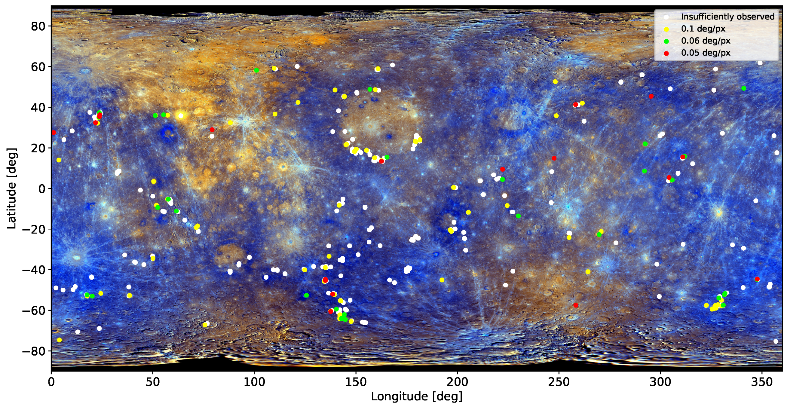
The data collected by past missions to Mercury does not allow the composition and property changes inside pyroclastic deposits to be unequivocally discerned. Therefore, we decide on the use of unsupervised learning techniques that do not require labels. Moreover, unsupervised learning is an exploratory approach capable of detecting patterns in large data sets without being conditioned. While classical machine learning techniques such as principal component analysis (PCA) have been traditionally used for this task, they present two shortcomings. First, they are linear architectures that lack the capacity to detect nonlinear patterns in the spatial–spectral data. Romero et al. [19] compared the performance of linear techniques and a deep learning network applied to Earth observation images and demonstrated the superiority of deep architectures in the extraction and classification of features. In addition, deep learning networks are versatile, serving various purposes like dimensionality reduction, target detection, or image generation. Hence, we opt for a deep architecture.

Deep learning approaches to treat HSI can be divided into techniques that work within the spectral domain, and techniques that simultaneously analyse the spatial and spectral domains [9]. In planetary observations, the spatial relationships between features often create patterns that can be correlated with spectral information (e.g., craters in an image). Selecting a spatial–spectral approach that can detect these dependencies increases the robustness of the classification and the significance of the features learned. These dependencies are expected to be crucial in the case study treated here, as highlighted by Besse et al. [15,17]. The convolutional autoencoder (CAE) is an architecture that can perform an unsupervised spatial–spectral investigation of HSI. The term convolutional refers to the use of layers that calculate the dot products between the input HSI and a moving kernel that outlines the image, extracting relevant features. This is a matrix operation between a kernel that is kept constant and a sub-set of the HSI with the same dimensions as the kernel. This architecture was first introduced by Chen et al. [20] for the classification of terrestrial images, and later improved by Ma et al. [7], Tao et al. [21]. The algorithm extracts the spectral and spatial features independently, which are then a combined input to the deep learning architecture for later classification. Mei et al. [22] extended this concept and presented a three-dimensional (3D) convolutional autoencoder, based on the 3D convolution introduced by Li et al. [23]. This architecture inspects the data in the spatial and spectral dimensions simultaneously, and has proved to outperform both supervised and unsupervised alternative techniques.

It must be noted that these techniques make use of the deep neural network for feature extraction, and then use a traditional clustering algorithm to classify each pixel. While some techniques embed the clustering step into the deep learning architecture, these are not adapted to HSI or 3D convolutions [24]. The development of such an architecture should be verified with the well-known Earth remote sensing data sets, a process which lies outside the scope of this work. Instead, we propose to base the architecture on the unsupervised three-dimensional autoencoder (3DCAE) proposed by Mei et al. [22], and we provide guidelines on how to tune the parameters to better train the network. The methodology followed in this work is illustrated in Figure 1 and detailed in this section.

2.1. Data Set

The MESSENGER mission delivered a wide variety of measurements that improved our understanding of geologic processes on Mercury. In this work, we focus on the study of explosive volcanic activity through a spectral investigation of the MASCS instrument’s data. MASCS is a point spectrometer, consisting of an ultraviolet and visible spectrometer (UVVS) covering the wavelengths from 115 to 600 nm with a 0.6 nm spectral resolution, and a visible and infrared spectrograph (VIRS) covering between 300 and 1450 nm with a spectral resolution of 5 nm [25]. In this work, we use the VIRS spectra available from the Planetary Data System (PDS) that has been radiometrically and photometrically corrected by the MESSENGER team as detailed by Izenberg et al. [4], and further calibrated by Besse et al. [15] to overcome the offset between the visible and near-infrared spectrum obtained through different instrument channels. The fully corrected spectra are retrieved from the Mercury Surface Spectroscopy (MeSS) database, a relational architecture that contains, for every MASCS footprint, the raw and corrected spectra, the associated geometrical descriptors, and relevant spectral parameters [26].

2.2. Data Preparation

For the methodology under consideration, using data from a point spectrometer is not ideal, since it does not output an HSI. However, the spatial coverage of the MASCS instrument is sufficiently high in some regions, allowing the individual spectral measurements to be processed into an HSI. To prepare the training data set, we define a bounding box around the geologic feature of interest from which to retrieve the spectral data. For our analysis of pyroclastic deposits, we defined a box that was 50% larger than the reported deposit size, to ensure that the feature was completely covered. When the deposit size had not been previously calculated, it was defined as five times the vent size. We applied a filter to remove the footprints with extreme observation conditions, where the topography could influence the measured reflectance. To this end, observations with incidence angles greater than ${75}^{°}$ and/or emission angles greater than ${80}^{°}$ were not included. Similarly, to prevent the effect of a high instrument temperature on the near-infrared detector, we only considered observations taken at less than $40{ }^{°}$C [14]. Finally, we cleaned up the data set from spectra with negative values or outlier reflectances larger than 0.2. Finally, to correctly construct an interpolated image, we ensured that the input measurements did not span several grid elements by defining a maximum footprint area of $25{\mathrm{km}}^2$.

To construct the HSI, we performed a spatial interpolation of the available data. We made use of the inverse distance weighted (IDW) technique, one of the most widely used interpolation algorithms that is available in most commercial Geographic Information System (GIS) software and that has proven to perform well in a variety of scenarios [27]. We modified this method to also consider the area of the measurement footprint. In this way, 80% of the interpolation weight was calculated based on the distance from the footprint to the grid element and 20% was calculated based on the area of the observation, prioritising smaller footprints.

Following this procedure we processed three sets of hyperspectral images with a spatial resolution of 0.1, 0.06, and 0.05 deg/px, covering 106, 76, and 45 of the identified volcanic vents, respectively. The distribution of these vents on Mercury is shown in Figure 2. As a final step in preparing the images for the input format to the 3DCAE architecture, the spectra were normalised to the range [0, 1], a common technique to avoid obstructing the numerical optimisation process [9].

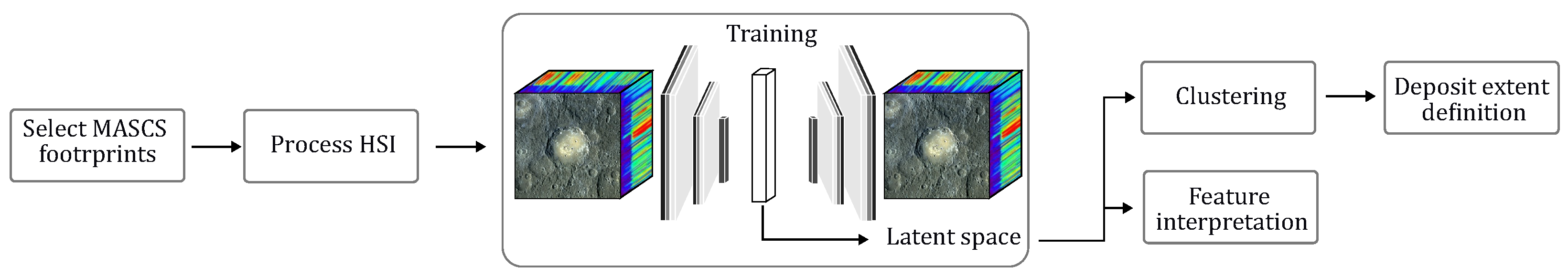
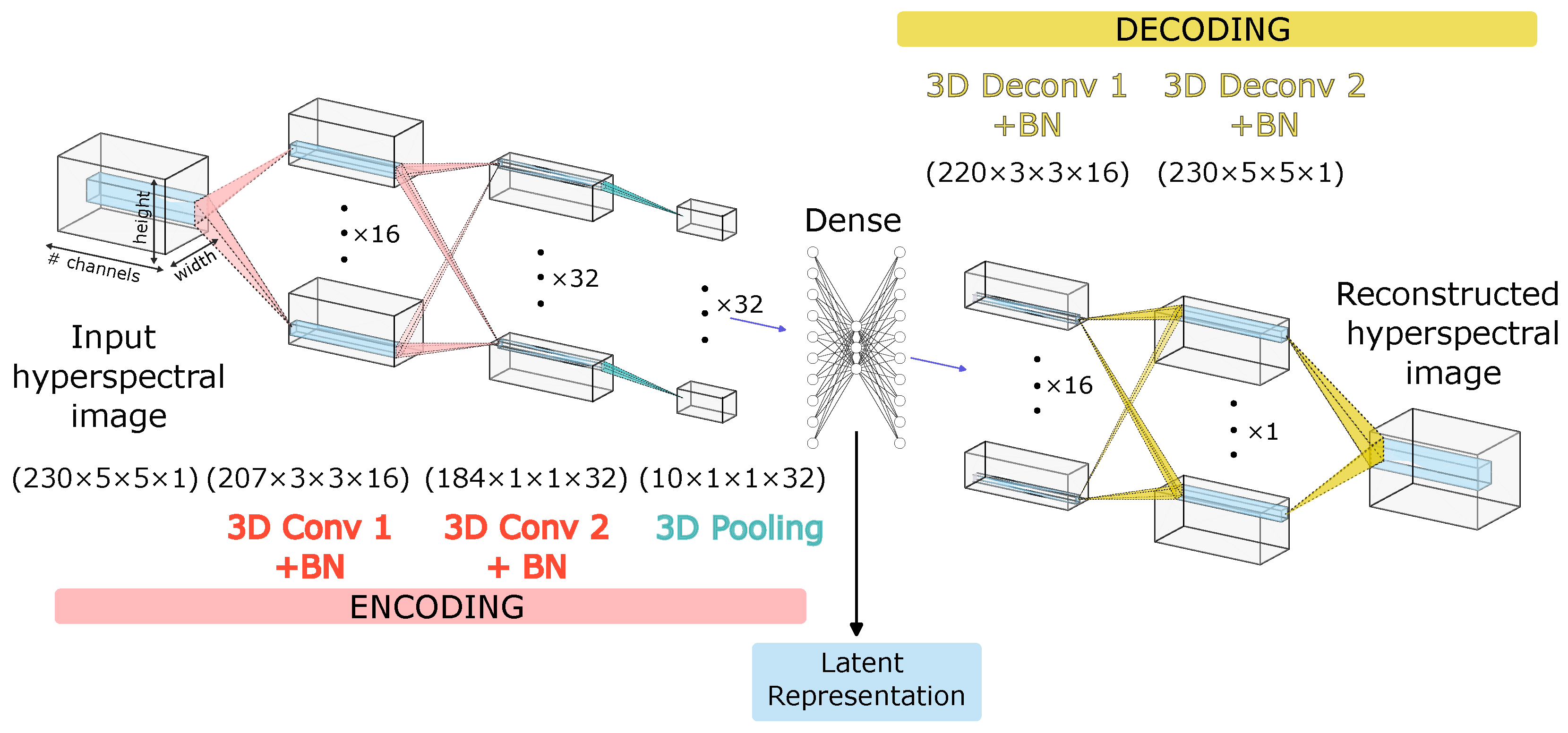
2.3. Deep Learning Architecture

Deep learning offers a unique perspective into the study of hyperspectral data, since it allows the spectral and spatial information contained in the images to be simultaneously explored and their dimensional complexity to be reduced. Moreover, the application of unsupervised techniques brings results that are not biased by human-made labels. In this work, we have adopted the unsupervised 3DCAE presented by Mei et al. [22] to explore the explosive volcanic deposits on Mercury. The working principle of an autoencoder is to learn the representative features from an input data set by first encoding the data into a lower-dimensional “latent” representation and then decoding this reduced representation aiming to reconstruct the input data. In this way, the error between the reconstructed and the input data is minimised, and the features learned are representative of the higher-dimensional information. Since we are dealing with three-dimensional (hyperspectral) images, three-dimensional operations are more efficient in capturing the spatial and spectral interactions. The construction of this architecture requires two different models, a training model and a test model. The training model consists of the complete autoencoder structure, with the encoder branch responsible for reducing the dimensionality through the extraction of relevant features in each layer, and the decoder branch inverting the encoder behaviour to output an HSI with the same dimensions as the input. This model is trained using the backpropagation method, minimising the loss function that calculates the difference between the input and output HSI. Once the training model is properly optimised, the testing model, which consists of the encoding branch with the optimised weights, is used for data reduction and feature extraction of the entire data set. The objective of the network is to extract, for each pixel, the relevant spectral and spatial features regarding the pixel itself and its surroundings. Therefore, the testing model is run pixel-wise and the output is a vector of length equal to the number of latent dimensions for each pixel. The input is a sub-patch of the HSI, centred at the pixel of interest and spanning the entire spectral range. The spatial dimensions of the patch determine the amount of spatial information available to the network and define the input size.

Regarding the complete autoencoder network, it is built as a sequence of layers. The encoder part consists of two convolutional operations of kernel size $24\times 3\times 3$ with a PReLU activation function that extracts features to a size (#channels × width × height × #filters) = ($184\times 1\times 1\times 32$). The convolutional operation acts in the three dimensions and the increasing number of filters enables the recognition of different patterns in the data. The dimensionality is then reduced following a three-dimensional pooling operation to size ($10\times 1\times 1\times 32$). This operation allows only the dominating features from the multiple filters obtained from the previous layer to be retained. Finally, the output from the pooling layer is flattened and connected through a dense layer. This ensemble of operations reduces the dimensionality from the original ($230\times 5\times 5\times 1$) size to a latent space ($n_{lat}$) of the chosen size. The decoder is built similarly, with two three-dimensional deconvolutional layers that reconstruct the latent representation to the original input size. The deconvolutional layers have kernel sizes of $9\times 3\times 3$ and $11\times 3\times 3$, and 16 and 1 filters, respectively. After each operation, a three-dimensional batch normalisation is performed to avoid large values in the feature space and ensure that the weights are not unbalanced. Figure 3 illustrates this architecture and the dimensions of the feature space at each layer. Adding a fully connected layer allows the latent space dimension, whose optimum value might change depending on the data under study, to be easily modified. This eliminates the need to use additional dimensionality reduction techniques such as principal component analysis (PCA). Once the network is trained, the encoder branch is isolated for the testing model. Whereas each pixel in the original HSI contained 230 spectral channels, the output of the testing model reduces this to $n_{lat}$ dimensions that incorporate spectral and spatial information. This information is then used to obtain cluster maps, where each pixel is assigned to a given cluster. For this step it has been determined that the k-means and bisecting k-means algorithms provide the best performance, and the latter is selected for this work.

3. Implementation of the Deep Neural Network

The implementation of the deep learning network is performed using the Keras (https://keras.io/, accessed on 7 July 2023) interface available on Python. It consists of a sequential model that is built by adding the layers described in Section 2. All layers are available through the Keras library and the hyperparameters (e.g., kernel size and number of filters) are set individually for each layer in the definition of the model. The architecture of a deep neural network is controlled by a large number of parameters that affect its accuracy, efficiency in extracting relevant features, and computational time. This results in an immense number of potential configurations that complicate the task of finding the optimum choice. To guide this process we restrict the tuning to the set of parameters that are more closely related to the type of HSI used and the scientific analysis of the results. The remaining parameters are set following the architecture recommended by Mei et al. [22]. These include the number of convolutional layers, the weight decay, and the learning rate. However, two important parameters in our study are the size of the input and output variables, which are assessed in more detail in this section. The ranges of values studied and the final configuration selected are presented in

Table 1. Parameter space for training the deep learning architecture. The parameters discussed in detail are bold.

Parameter	Range Studied	Final Configuration
Patch Size	5–15	5
Latent dimension	9–80	20
Number of filters	16–24	16
Number of layers	2	2
Learning rate	0.01	0.01
Weight decay	0.005	0.005
Test/Train ratio	0.8/0.2	0.8/0.2
Number of clusters	4–15	8

.

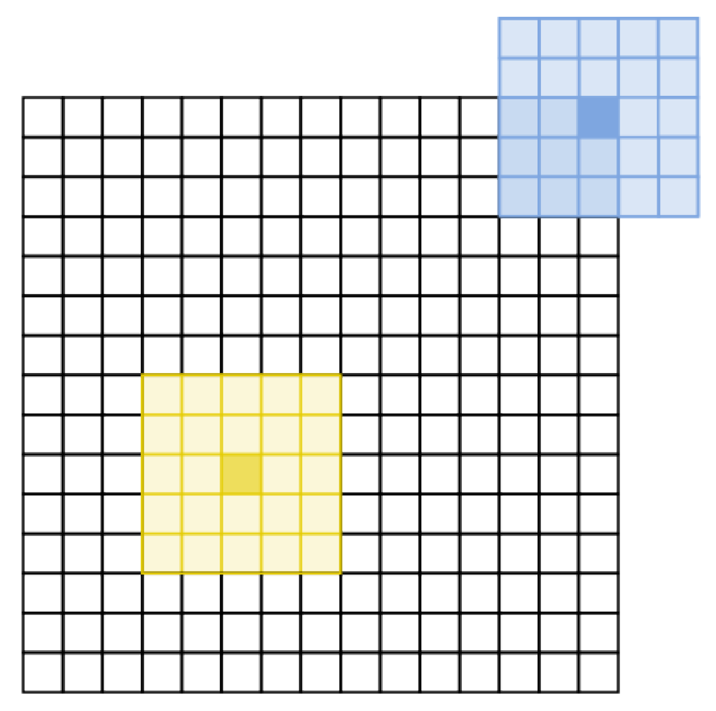
3.1. Selection of the Input Size

The objective of the neural network is to extract relevant information of each pixel and its surroundings. To include the spatial information of the surroundings, the original image is divided into patches. When applying the methodology for an HSI with spatial dimensions $d_1\times d_1$, the input will be formed by $d_1^2$ patches, one for each pixel. A patch is defined as a sub-division of the HSI centred at each pixel with spatial dimensions $s\times s$ and spanning the entire spectral domain, as illustrated in Figure 4. In the case of the bordering pixels, the data to form the patch is incomplete. In this study, this is not an issue, since there are observations beyond the limits of the hyperspectral image that allow the patch to be constructed. If this is not the case, alternative solutions should be studied, such as mirroring the corner information. The patch size regulates the input size and the amount of spatial information that is fed to the neural network. A patch size of one is equivalent to running the algorithm with independent spectral measurements. By increasing this variable we include more spatial information, allowing the network to learn a greater number of features in this dimension. The optimum patch size for a given study case will depend on several factors such as the number of spectral channels, the spatial resolution, and the spatial scale of the phenomenon under study. For this application, we test the effect of varying the patch size from $5\times 5$ to $15\times 15$ pixels. It is found that the configuration with a larger patch size outputs less detailed cluster maps that reflect some larger-scale spatial features such as crater rims. However, with this configuration some smaller-scale details are overlooked. Therefore, in this study we select a patch size of $5\times 5$. This configuration allows spectral features to be detected that are otherwise dismissed, while still considering the spatial context.

3.2. Selection of the Output Size

The output dimensions of the proposed architecture are defined by the dimensions of the latent space ($n_{lat}$) and the number of clusters ($n_c$). This is a crucial pair of parameters that will affect the overall performance of the algorithm and the capacity to interpret the results. Generally, a larger latent space will be more accurate in reconstructing the input but less efficient in extracting relevant features. Moreover, clustering algorithms become inaccurate when dealing with high-dimensional data, since the differences in distances between data pairs decrease (a phenomenon referred to as the curse of dimensionality [28]). Therefore, the number of latent dimensions will not only affect the interpretability of the extracted features, but also the quality of the clustering results. The number of clusters is selected based on the performance, but under the requirements of this specific study case. In this scenario, to capture the inter- and intra-facula variations that characterise the pyroclastic deposits, at least eight clusters are required in total (half of them will predominantly identify the background terrain). To define the optimum number of latent dimensions and clusters, we look into the effect on the clustering performance, assessed through the silhouette score [29]. This performance parameter ranges from −1 to 1, with −1 indicating the worst clustering performance and 1 indicating a dense clustering, and a silhouette score of 0 referring to overlapping clusters. As illustrated in Figure 5, there is a decreasing trend in the clustering accuracy with an increasing number of clusters, which stabilises after 11 clusters. Considering this, the number of clusters is set to eight to satisfy the requirement previously imposed. Taking into account these results, the optimal number of latent dimensions is 20, followed closely by 15. At the risk of obtaining redundant features, the number of latent dimensions is then set to 20 to ensure that all relevant features are extracted.

3.3. Training and Performance Evaluation

We perform the training of two separate models, for the data sets with 0.1 and 0.06 deg/px, respectively. The input data set for training contains approximately 50,000 samples, which consist of individual patches of the HSI extracted from the regions of interest containing the pyroclastic deposits. The training data set also contains samples of background material from different spectral units of Mercury. The input samples are divided, using 80% for training and the remaining 20% for validation. The model is trained for a total of 15 epochs, and it is observed that after 4 epochs the loss and the validation loss stop decreasing. The trained model presents a training loss of 0.0014 and a validation loss of 0.0047 for the data set with a 0.1 deg/px, computed based on the mean squared error (MSE). For the data set with a 0.06 deg/px resolution, the training loss is 0.0018 and the validation loss 0.0027. These values support that the model performs well, also on validation data. These results are comparable to the errors found by Zhao et al. [30] for the application of a similar architecture to Earth observation HSI. We tested the effect of modifying several hyperparameters such as the learning rate, the number of filters, and the kernel size, and we arrived at the values discussed in Section 2.3. Once the final architecture was established and the autoencoder was trained, the test model formed by the encoder branch was applied to extract the features for each pixel in the input HSI.

4. Results

The trained neural network is applied to the entire data set of HSI of the known faculae, composed of a suspected explosive vent and its associated pyroclastic deposit. The vent consists of an irregular pit without raised rims. Depending on the morphology, different types of vents have been defined, namely: simple vent, pit vent, and vent with mound [16]. Moreover, while in some cases the vents are isolated and formed by a single eruption event, Pegg et al. [18] discussed that most of the vents are formed by multiple explosions, creating so-called compound vents. The deposits surrounding these vents are typically characterised by a high reflectance and a red spectral slope, diffuse margins, and spectral properties that vary with the distance to the vent [14,15]. This contrasts with pyroclastic deposits on the Moon, which are characterised by their low albedo compared to the background terrain [31]. When comparing the absolute value of the pyroclastic deposit albedo, the Hermean and lunar deposits fall within the same range [2]. The difference in apparent behaviour is due to the darkness of Mercury’s surface. To date, more than 180 pyroclastic deposits have been identified on Mercury, some of them associated with multiple vents [5,12,16]. A spectral investigation of a sub-set of these features has highlighted the variability across deposits on Mercury, and also within a given deposit [17]. Altogether, the volcanic vents and associated deposits present a wide diversity of morphological and spectral characteristics. While previous studies have focused on the analysis of individual aspects of this variability, a combined analysis is more suitable to constrain the dependencies between different factors causing it (e.g., multiple explosions, deposit age, composition, link with background material, etc.). In particular, the effect of the background material on the properties of the deposit due to mixing is a limitation from previous studies that we can overcome with the methodology developed here. We follow two approaches to analyse the data. First, we apply a clustering algorithm to the reduced latent dimension that classifies every pixel in the HSI using the spectral and spatial information extracted by the algorithm. For the study of pyroclastic deposits, this information is used to characterise the extent of the deposit and study the inter- and intra-deposit variability. Using the cluster maps, we can visualise the deposit irregularities and better constrain the extent and, therefore, the volume of volatiles involved in these eruptions. However, the analysis of the clusters by themselves does not provide an insight on the features learned by the algorithm. To analyse this, a second approach is followed, which consists in exploring the deep learning filters and the latent dimension. We look for patterns that we can correlate with physical and spectral properties and ultimately relate them to the composition and the surface processes that affected the deposits. Finally, using the cluster maps we isolate the pyroclastic deposits from the background terrain and we obtain the deposit area.

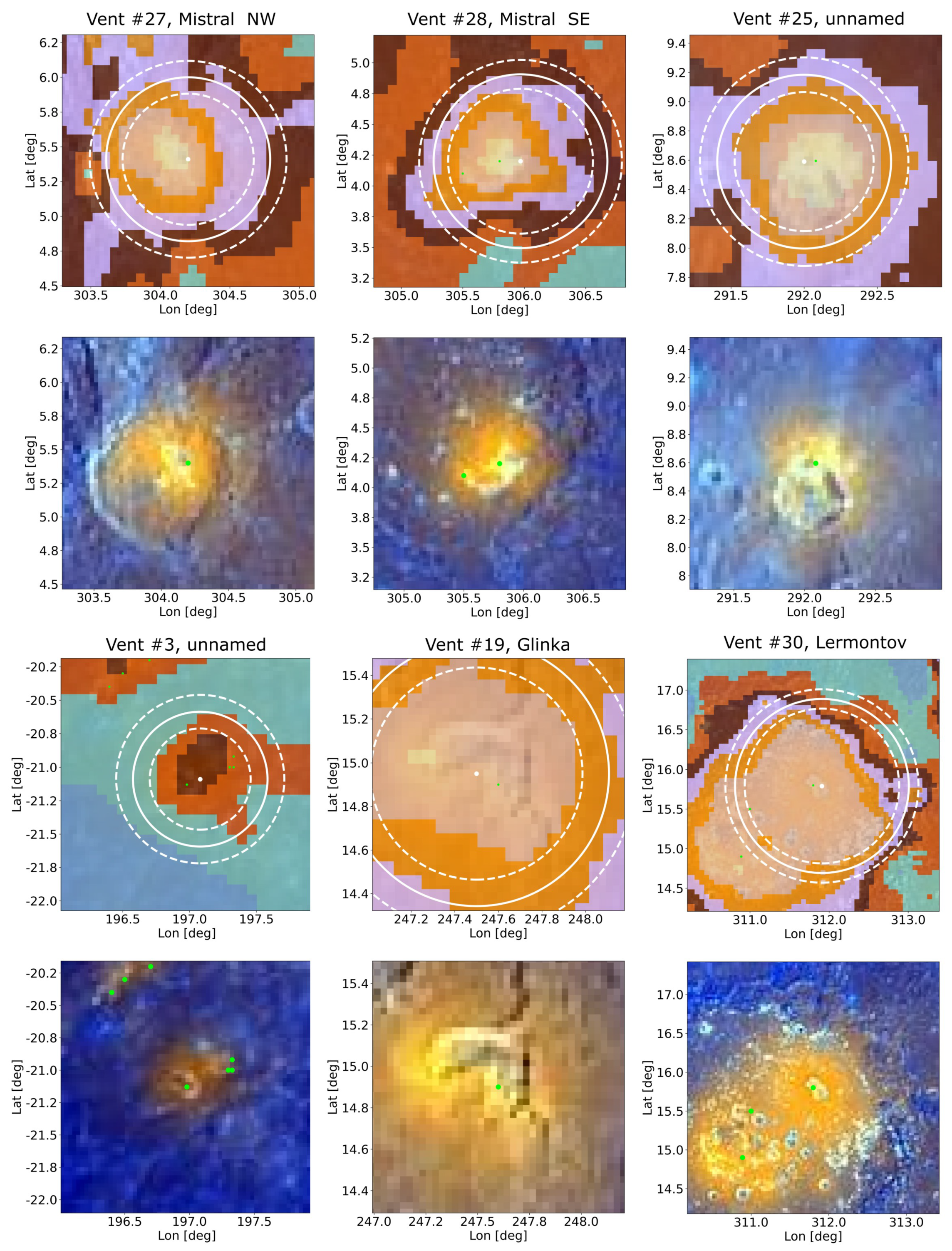
4.1. Cluster Maps of Pyroclastic Deposits

By setting the desired number of clusters, the algorithm categorises each pixel in the HSI as part of a given cluster, based on the latent dimensions extracted from spectral and spatial information. Figure 6 shows the average spectrum of each cluster, ordered in descending reflectance. The average reflectance spectrum of Mercury, as provided by [26], is displayed in a black dashed line, which closely matches the reflectance of cluster 5. We note this cluster as a reference for the average properties on Mercury, while taking into account that the properties of a given deposit will largely depend on the local background terrain [14]. There are four clusters above the average reflectance and three below it. This is expected since pyroclastic deposits are usually characterised by a high reflectance, and therefore, the data set used contains a large amount of high-reflectance spectra. The clusters related to darker spectra are due to the fact that we include data from the deposit background. We observe that the error bars from different clusters overlap. This is explained by the fact that the clustering is not based on the reflectance spectrum of each pixel, but on the extracted features from the pixel and its surroundings. Nonetheless, due to the flatness and lack of absorption bands in Mercury’s spectra, the main spectral parameters that can be extracted are related to the reflectance and spectral slopes. Therefore, by limiting the number of clusters to eight, these are the parameters that drive the clustering.

Previous studies have highlighted that pyroclastic deposits have characteristic spectral properties in the UV, visible (VIS) and NIR domains (i.e., a pronounced downturn in the UV domain, a higher VIS and NIR spectral slope, and a high reflectance) [5,15,17,32]. However, these properties are not ubiquitous and the large variability between different faculae makes it difficult to define a single framework to characterise these features and limit their extent. Moreover, pyroclastic deposits are diffuse and the spectral properties change with the distance to the vent, and depending on the type of background terrain. The cluster maps become an efficient tool to visualise the inter- and intra-variability in the faculae. Due to the diffuse nature of the deposits, in the cases where the deposit exhibits a distinct spectral behaviour compared to the background terrain, the clusters form concentric structures, centred at the location of the vent and extending until the deposit blends with the background terrain. These concentric structures, which resemble rings, follow a trend of decreasing cluster number (corresponding to a decrease in reflectance and VIS slope) with increasing distance to the vent. The limit of these concentric rings with the homogeneous cluster defining the background terrain can be used to define the extent of the deposit. The variability in the faculae is reflected in the cluster maps. The cluster ring structure is not always present, since not all deposits exhibit a clear spectral signature. When the ring structure is present, it can be circular (which is the expected result from an isolated vertical eruption in an airless planet like Mercury) or irregular. An irregular ring structure can highlight interactions with the topography, overlap from multiple eruptions in proximity, or a more complex eruption process.

Although the concentric ring structure is a useful tool to visualise and characterise the pyroclastic deposits, this is not a ubiquitous phenomenon and, therefore, it cannot be used as the unique method to identify or delimit the extent of a facula. For example, in the case of the oldest explosive volcanic eruptions, the spectral signature of the deposit can be faint or nonexistent, and therefore, the cluster maps will lack the concentric ring structure that clearly highlights the deposit from the surroundings. From the 106 volcanic vents studied with a spatial resolution of 0.1 deg/px, 26 lack any type of layer structure. These pit sites are often located in areas of very low or very high-reflectance background material. The remaining pit sites reveal concentric ring structures of the clusters, which relate to the change in properties of the pyroclastic deposit with the distance to the vent, as the deposited layer diffuses, blending with the underlying material. However, the concentric structure itself can take multiple representations. In 18 of these pit sites, the deposit is only distinguished from the background terrain with a single layer. In these cases, the spectral properties are sufficiently similar across the deposit to be classified into the same cluster. While this still provides information on the extent of the deposit, the fact that 40% of the deposits have been found to lack a multi-layer structure precludes this attribute from being used as a facula identification criterion. From the remaining pit sites that show a multi-layer structure, 36 are located in proximity to other pits and subsequently produce overlapping deposits. In these cases, the multi-layer structure is irregular, with multiple foci pointing at the location of different vents. Finally, from the 106 pit site cluster maps, only seven show a circular multi-layer structure. Therefore, the assumption of a circular deposit used by Kerber et al. [13] and Barraud et al. [14] will be inexact in most of the cases and will lead to inaccuracies in the calculation of the volume of volatiles driving the eruption. This is nonetheless a good initial approximation to explore faculae when the data set is limited.

Figure 7 illustrates the cluster maps for six well-known faculae, where the colouring standard follows the convention from Figure 6. In this image, the identification of the deposits from the cluster maps is compared side by side with the size estimates developed by [14] for a circular deposit and with the MDIS false-colour map of the region. The first trait that stands out is the multi-layer structure that has been discussed and that is present in all six faculae. The central cluster in these layers usually corresponds to the location of the vent and to the bright area on the enhanced colour map. Although the cluster maps share this common multi-layer structure, they present differences that can be used to quantify the variability between pyroclastic deposits. Regarding the spectral properties of the deposits, we observe that the unnamed vent #25 and the Mistral NW and Mistral SE deposits present similar characteristics, with cluster 1 at the centre of the multi-layer structure and a sequential decrease in clusters in thin layers until the background terrain. The Glinka and Lermontov deposits are slightly different, with the predominance of cluster 2, followed by the same sequential decrease in clusters. However, the unnamed deposit #3 is spectrally different, and this results in the central layer corresponding to cluster 5, rather than clusters 1 or 2. In this case, the background terrain corresponds to darker material and the deposit itself is darker. The dependence of the properties of the deposit on the properties of the background terrain supports the value of using a technique that considers both the spectral and the spatial domains. This dependence was already highlighted by previous studies (e.g., Barraud et al. [14]) and the methodology followed allows the extent of the faculae to be properly defined and to characterise the background terrain. Second, we can compare the size of the deposits assuming a circular shape with the extent of the deposit delimited by the extent of the concentric multi-layer structure. We note that the comparison is not straightforward due to the irregular shape of the deposits, especially in the case of the Lermontov facula. However, we observe that in most of the cases the extent of the facula lies between the error bars defined for a circular perimeter. The match is especially good for the unnamed vent #25 and the Mistral NW and Mistral SE deposits, which have a clearer spectral signature with a large occurrence of the high-reflectance cluster 1. Moreover, we note that the extent delimited by this technique exceeds the area calculated based on the visual inspection of the enhanced colour image by [13], following the trend observed by Barraud et al. [14]. In the case of the Glinka deposit, it is slightly larger, according to the cluster maps, than previously identified. In the cases of the unnamed vent #3 and the Lermontov facula, due to the slightly elliptical shape of the deposits, the extent delimited by the cluster maps lies closer to the lower or upper bounds of the radius depending on the azimuth.

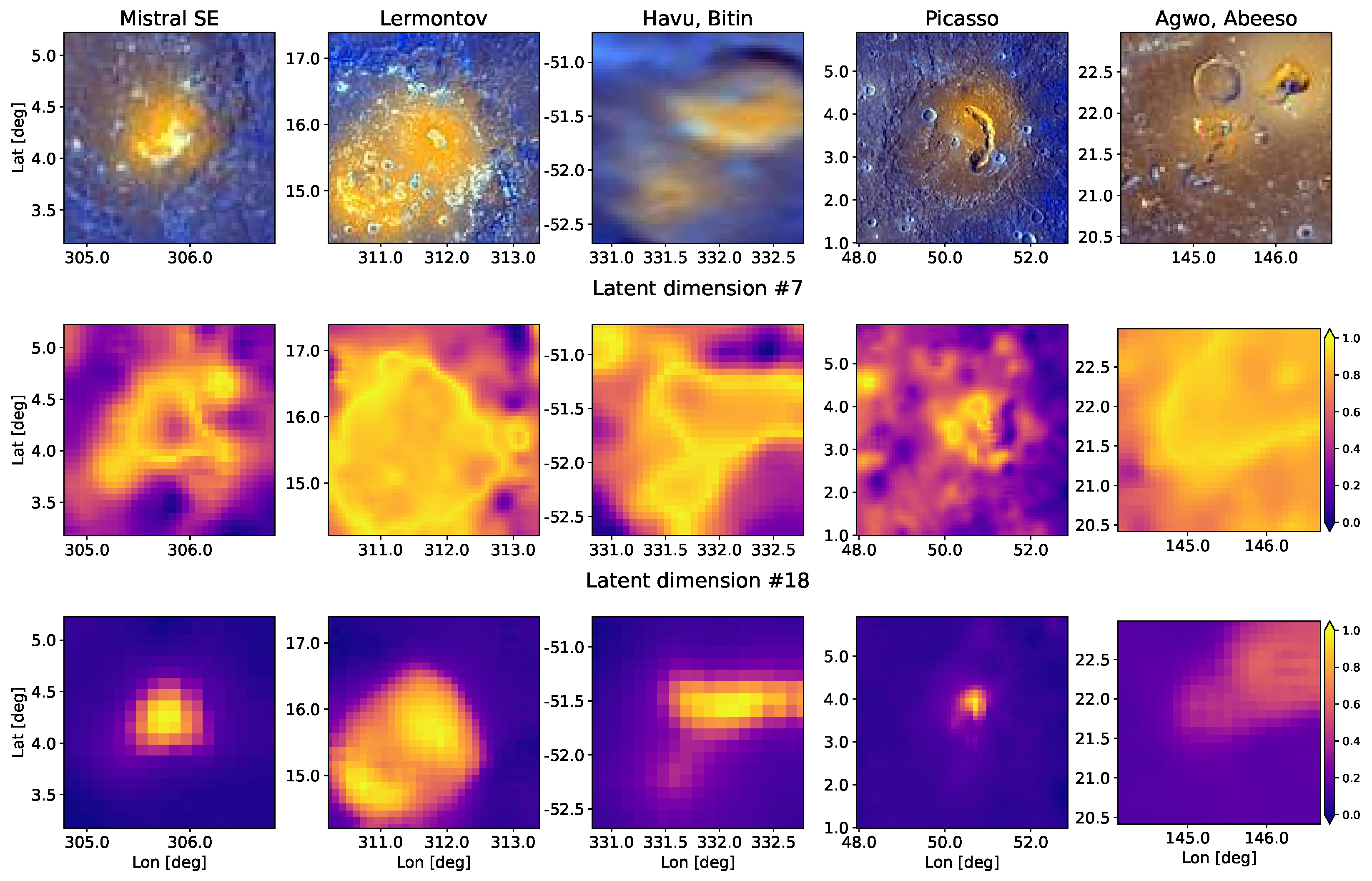
4.2. Feature Extraction

The result of the dimensionality reduction performed by the deep learning algorithm, the so-called latent space, contains information about the most important features that characterise the input HSI and will drive the clustering process. Although investigating the extracted features is not straightforward, it offers a possibility to dive into the otherwise black box process that is the 3DCAE. In this analysis, we will focus for simplicity on the results for the case with 0.06 deg/px resolution.

We correlate each latent dimension with the MASCS reflectance spectra to gain insight into which wavelengths are mainly dominating the data reduction. These results are depicted in

Table 2. Latent dimensions with the highest correlation to MASCS reflectance at specific wavelengths ($\lambda$).

Dimension	1	2	3	4	10	11	12	13	14	15	16	17	18	19	20
$\lambda$ (nm)	1360	785	1060	765	1290	1210	725	1180	770	770	775	1050	1070	1210	1210
Correlation	0.92	0.96	0.95	0.96	0.93	0.95	0.93	0.95	0.92	0.96	0.96	0.95	0.93	0.95	0.96

for the latent dimensions that show a high correlation (>0.9) with the reflectance at specific wavelengths from the MASCS/VIRS spectral range. The first observation is that the dimensionality reduction process appears to be compressing the information from the VIS and NIR spectral ranges, with specific reflectances starting at 725 nm and ending at 1360 nm, but not in the UV, which could suggest that the reduced dimensions are mainly derived from this spectral domain. This is initially surprising, since multiple previous analyses have highlighted the tendency of pyroclastic deposits to present a pronounced UV downturn [5,14]. However, we further investigate the correlation between each latent dimension and the spectral slopes in the UV, VIS, and NIR domains, and we find that there are four latent dimensions (number 2, 4, 15, and 16) that have a high correlation with the UV slope. We conclude that while the information in the VIS and NIR domains is compressed from specific wavelengths, in the UV range it is mostly the slope that will dominate the compression. Second, we note that multiple latent dimensions present a very high correlation with specific wavelengths in the NIR domain. In Figure 6, we observe that the NIR spectrum is more noisy and presents consistent bumps in reflectance at given wavelengths. Further investigation is required to discern if the DL network is highlighting this noise in the NIR spectral range, or if it is highlighting a behaviour specific to pyroclastic deposits.

Moreover, we test the relation between the latent dimensions and several spectral parameters that characterise the data. We start with the spectral parameters previously defined to study pyroclastic deposits by Goudge et al. [5], Besse et al. [17], and Barraud et al. [14] and continue by testing the correlation with a custom set of parameters. For the previously defined parameters, we consider the slopes in the VIS and NIR domains, which are known to decrease with increasing distance from the vent in pyroclastic deposits; the curvature, which is known to be associated with the presence of hollows and young material [33,34]; and the UV downturn. The newly defined parameters are based on the spectra that produce extreme values for the latent dimensions, and therefore, are suspected to play an important role in the extraction of features from the original data. These are the slope in the UV and the change in slope between two spectral regimes, namely, the UV/VIS slope break defining the difference between the spectral slope in the UV and VIS domains, and the VIS/NIR slope break for the same difference between the VIS and NIR domains.

From

Table 3. Highest correlation between set of spectral parameters and latent dimensions.

Parameter	VIS Slope	NIR Slope	Curvature	UV Downturn	UV Slope	UV/VIS Slope Break	VIS/NIR Slope Break
Correlation	0.8	0.58	0.75	0.18	0.92	0.6	0.76
Dimension	11	1	8	11	4	4	9

, we notice that the largest correlations are found with the spectral slopes in the UV and VIS domains, respectively. This is expected since the spectrum of Mercury lacks absorption bands and, therefore, the spectral slopes are the first parameter that characterise these measurements. For the NIR slope the correlation is less evident, which is consistent with the lower quality of the spectrum in this domain and the lack of characteristics identified in this domain do date. It is interesting to verify that there is one latent dimension correlated with the curvature, which confirms that this characteristic becomes a factor in the clustering process. This could be due to the presence of hollows in some of the deposits used for training the algorithm, or to the fact that the pyroclastic deposits themselves can have a higher curvature than the crater floor.

Regarding the newly defined parameters, we observe in Table 3 that the VIS/NIR slope break is correlated with the latent dimension #9, which also shows a moderate correlation with the curvature. This behaviour is consistent with the spectra of fresh units such as impact ejecta and hollows, which present a curved spectrum in the UV–VIS domain and a less steep slope in the NIR domain [34].

For the latent dimensions that do not present a strong correlation with the independent reflectance, we investigate whether spatial patterns are being highlighted. As mentioned, the properties of the pyroclastic deposits change with the distance to the vent, becoming closer to the background terrain as the diffuse limits of the deposit approach. This is identified in the cluster maps by the concentric layers following the shape of the deposit, centred at the location of the vent. This spatial gradient makes the deposits identifiable from the spatial domain in addition to the spectral domain. We study this possibility through two latent dimensions that appear to capture this behaviour. First, we analyse the example of latent dimension #7, which has a correlation of 0.72 with the reflectance spectra, a notably lower value than for the dimensions summarised in Table 2. Figure 8 shows multiple examples of the maps of this specific latent dimension compared to the MDIS image of the terrain. From a visual inspection, the latent dimension appears to highlight the border of the deposit. This is a unique output of the DL architecture, since the border of the deposits cannot be found with the current topological information that we have of the planet. Moreover, the deposits present a different extent when looking at different wavelengths. This leads to an underestimation of the dimensions of the deposit extent when defined based on MDIS colour images, which only include 11 spectral channels. Moreover, the DL network does not define these boundaries based on individual wavelengths, but rather based on a nonlinear combination of all the spatial and spectral parameters introduced. Therefore, although with this approach we lose interpretability, we gain a new insight into the data. It is interesting that this behaviour is independent of the brightness of the deposit, nor is it highlighting a specific reflectance. This leads us to think that the neural network is detecting the deposit boundaries at the pixels where the gradient of spectral properties is closer to zero. That is, the algorithm is taking into account the change in spectral properties between adjacent pixels in all directions and extracting as a feature the outline of minimum change that determines the boundary between the deposit and the underlying terrain. Using this information together with the spectrally dominated features as an input for the clustering increases the robustness of the procedure and the reliability of the cluster maps. Second, we look into the example of latent dimension #18 from the data set with a 0.1 deg/px resolution. In this case the correlation with the reflectance spectra is 0.81, which indicates that spatial information might be conveyed in this dimension. Looking at the maps of this latent dimension in Figure 8 we observe a very high contrast between the deposits and the background terrain. In this case, independently of the specific brightness of the background terrain and the variations within a given deposit and between deposits, the background pixels have normalised values very close to zero. This behaviour is observed in a wide variety of terrains, from the low-reflectance material (LRM) that surrounds the Picasso crater to the high-reflectance red plain (HRP) unit surrounding the Agwo and Abeeso faculae. In comparison, the pyroclastic deposits are clearly distinguishable from the surroundings. Up to now, due to the wide inter- and intra-variability in the pyroclastic deposits, it has not been possible to unequivocally identify the deposit from the surroundings. By inspecting individual reflectances, there are no clear criteria that separate pyroclastic deposits form other terrains. This latent dimension offers a new methodology to identify the presence and extent of pyroclastic deposits. This can be extended to the entire map of Mercury to look for this signature in other regions.

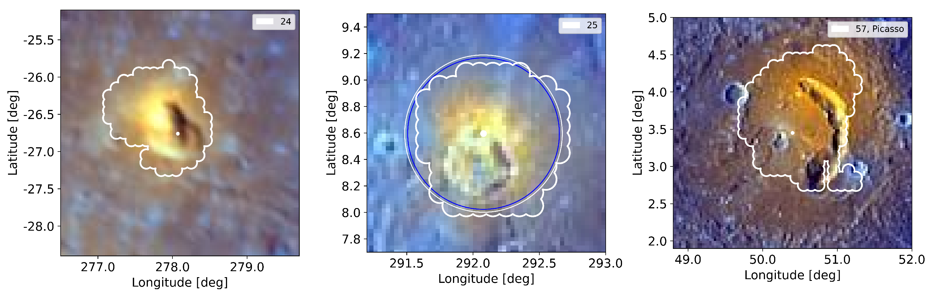
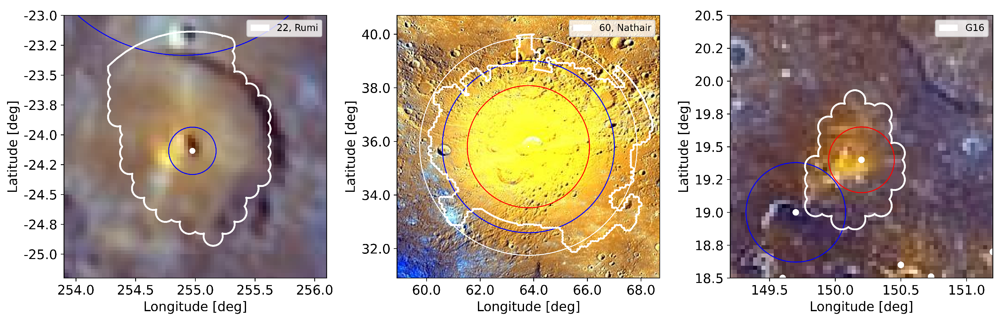
4.3. Pyroclastic Deposit Area

Assessing the extent of pyroclastic deposits bears implications for our comprehension of Mercury’s volcanic history and the planet’s thermal and geochemical evolution. The deposit size relates to the volatile contents required to emplace the pyroclasts at such distances [35]. Furthermore, the challenge lies in distinguishing the spectral signature of the pyroclastic deposits from the surrounding terrain. Delimiting the deposits enables us to obtain a more precise spectrum of the background terrain which then serves as a basis for normalisation when comparing the characteristics of various deposits. Finally, obtaining the shape of irregular deposits, coupled with an understanding of the vent morphology, can help in identifying whether a volcanic eruption occurred at an oblique angle. The cluster maps become an effective tool to define the extent of the deposit when the facula is spectrally distinct from the surrounding terrain. In such cases, the cluster map highlights a concentric ring structure, which can be circular or irregular depending on the deposit shape. Using as a boundary the outer layer of this concentric structure, we define the extent of the pyroclastic deposits and calculate the deposit area. When the deposit is isolated, this boundary can be automatically extracted. However, when the deposit is in proximity to other regions with similar spectral characteristics, the boundary formed by the outer concentric cluster layer can be connected to these other regions. This is the case for vent #27 illustrated in Figure 7, where cluster 4, coloured in pink, defines the outer layer of the concentric structure but shows some ramifications connected to adjacent areas. In such cases the deposit extent cannot be automatically extracted and we manually crop the out-flowing regions. When available, we use the maximum radial extent of the deposit defined by Barraud et al. [14] to define the cut radius threshold. Since this procedure can be subject to interpretation, we provide both the original and the modified shapefiles, available at Leon-Dasi et al. [36]. In Figure 9, we provide three examples of the deposit extent defined using this methodology. Due to the low spatial resolution of the cluster maps, the border is not smooth and presents a step-like pattern instead. In the case of symmetric and well-defined deposits such as #25, the extracted extent does not differ largely from the radius estimated by Barraud et al. [14]. However, in more irregular deposits such as #57, assuming a circular shape would largely overestimate the deposit area.

There are two limitations that affect the number of deposits that can be characterised using this methodology. First, the deposit needs to be sufficiently covered with MASCS footprints to form an HSI with the required resolution. Second, the deposit has to be spectrally different from the surroundings in order to present the characteristic concentric cluster layer structure that we use to define the extent. Moreover, if the deposit extent is too small to be resolved as a concentric layer structure with the spatial resolution of 0.1 deg/px used in this methodology, it will not be properly detected. We define the extent of 35 isolated deposits and 20 deposits formed by multiple vents, which overall cover 110 vents. From these 55 deposits, 36 have not been previously measured with techniques other than visual inspection from MDIS false-colour images, and 17 have not been previously studied.

Table 4. Deposit area of isolated pyroclastic deposits. Equivalent vent IDs extracted from Jozwiak et al. [16], Goudge et al. [5], Kerber et al. [13], Barraud et al. [14] and Pegg et al. [18].

ID	Equivalent Vent ID	Host Crater/Facula Name	Lon (deg)	Lat (deg)	Deposit Area (km${}^2$)
					Barraud et al. [14]	Kerber et al. [13]	Goudge et al. [5]	Thomas et al. [12]	This Work
2	J2, G11	Brooks	−167.6	−45.04			484		153
6	J6, G7	Tolstoj	−161.14	−19.88			512		326
13	J13		−137.79	4.43584					1020
15	J15, B15		−136.79	−3.54	11,310			23,181	7721
16	J16		−135.49	−8.41					790
17	J17		−129.99	−13.53					849
19	J19, K29, B17	Glinka	−112.4	14.9	1963	846		1730.98	2398
20	J20, K10	To Ngoc Van	−111.8	52.6		2924		532.02	2907
22	J22	Rumi	−105.024	−24.13				186.4	2712
23	J23	Matisse	−89.21	−21.22				163.1	3407
24	J24		−81.93	−26.76					2272
25	J25, B18		−67.92	8.59	1963			1820.98	1994
26	J26, K26	Catullus	−67.5	22		921		1648.26	2490
27	J27, K33, B1	Veronese	−55.8	5.4	1963	421		2847.89	2662
32	J32, K22, B27	Enheduanna	−33.7	48.4	3848	1111		1875.55	818
33	J33	Namarjira	−32.9	58.8			1352		292
37	J37, K16, B21	Geddes	−29.5	27.2	2827	1654		2331.53	953
54	J54		24.41	−51.66				1961.56	1193
57	J57, K37	Picasso	50.4	3.45					4323
60	J60, K1, B8	Nathair	63.8	35.8	61,575	19,466		38,589.11	51,760
61	J61		65.74	−15.56					1836
110	P18		−4.1	26					298
142	P82		54.9	−11.2					1361
146	P92		62.4	−11.5					744
148	P101		51.8	−8.3				738.98	1649
184	P162		144.8	−59.4					333
187	P166		110.4	58.8					176
190	P169		121.1	60.1				3088.54	239
193	P184		144.8	−64.5					1117
237	P290	Matisse	−90.2	−22.7	6362			4214.96	6895
240	P198	Hesiod	−34.6	−59.4					194
252	P347	Mussorgskij	−97.6	33.1					710
278	P402	Zmija	92.3	−37.7					655
327	T5014	Neruda	125.65	−52.56	5027				2705
369	T6125		−56.09	3.76				89.9	90

summarises the results for the isolated deposits and

Table 5. Deposit area of pyroclastic deposits formed by multiple vents.

Group ID	Vent IDs	Host Crater/Facula Name	Lon (deg)	Lat (deg)	Deposit Area (km${}^2$)
					Barraud et al. [14]	Kerber et al. [13]	Goudge et al. [5]	Thomas et al. [12]	This Work
G2	282, 283, 261, 131, 260, 391		22.75	36.3				1731	1109
G3	50, 150, 151, 328	Nahaki	17.71	−52.71	6362			3230	2475
G9	59, 145	Neidr	57.3	36.1			4273		3664
G11	65,156, 157, 158	Alver	76.16	−66.78				10,127	1585
G13	68, 345	Becket	111.2	−40		408			753
G15	89, 90, 168, 269	Agwo/Abeeso	145.8	21.8	10,210	4938		3678	7982
G16	96, 171		149.6	18.5		317			930
G22	72, 73, 74, 76, 77, 192, 339	Sher Gil	134.81	−45.45					408
G27	93, 94	Vazov	147.86	−65.15				431	422
G31	1, 225,226, 227, 228, 229, 275, 385	Slang	181	24.3		10,414			4249
G37	3, 234, 362, 363		196.98	−21.13	1257		524	4089	2117
G45	28, 288	Mistral	305.8	4.2	2827	1245		2548	3405
G50	34, 242, 243, 244, 245, 317, 318, 319, 320, 321	Pampu	328.3	−58	6362	4950			4873
G51	36, 324	Ular	330	−55	5027	2079		4363	3048
G52	35, 325	Sarpa	329.1	−53.2	3848	2233		2957	2354
G53	38, 329	Havu	331.4	−52.2	1257	453			842
G54	248, 249, 334	Bitin	332.1	−51.4	3848	1021		4363	1725
G55	30, 105, 378	Lermontov	311.4	15.5	15,865	6980			13,496
G58	70, 210, 346		124.80	−40.09					440
G59	106, 387, 388	Praxiteles/Orm	−60.27	25.96	5654	3804		11,484	5295

for the deposits with multiple vents. In each table, we provide the vent IDs as identified in the Supplementary Material, the deposit area calculated by previous studies if available, and the area calculated in this work. In the case of the group deposits, the vent IDs identify all the vents that fall within the extent of the deposit, and the location coordinates correspond to those of the vent closer to the centre of the deposit. In the cases where previous authors consider the facula to be multiple separate deposits (e.g., Lermontov), the deposit area calculated by these studies is reported as the addition of the individual deposits included in the group.

5. Discussion

5.1. Evaluation of the Deposit Extent

Providing an accurate definition of the pyroclastic deposit extent is essential to estimate the eruption velocity and the volatile content required to achieve the observed dispersion. The adopted methodology introduces a major advantage with respect to previous techniques that relied on the visual interpretation of false-colour mosaics derived from PCA components. Pyroclastic deposits present a change in behaviour depending on the spectral domain which results in a different apparent extent depending on the wavelengths that are considered. This leads to an underestimation of the deposit size when analysing the false-colour mosaics, as reported by Barraud et al. [14]. Including all the spectral and spatial information becomes a high-dimensional problem that is difficult to tackle with traditional data analysis techniques. The use of a deep neural network to extract the relevant features has allowed us to include in a single latent space the information contained across the spectral domain and the spatial variation in the spectral properties. This feature extraction is nonlinear and has proven capable of recognising spatial patterns such as the border of the deposits with the background terrain. As a result, similarly to the work in Barraud et al. [14], the area of multiple deposits has been calculated to be larger than in previous studies that relied on the visual identification from images that contain information from the visible domain [5,12,13]. In Figure 10, we provide three examples of this effect. In all three cases we observe that the spectral signature identified from the false-colour images does not reach the identified edges of the deposit. This is particularly evident for the Nathair facula in the central figure, where the identified deposit boundaries match the maximum radius calculated by Barraud et al. [14], confirming the underestimation of previous studies.

In several instances, the calculated area is found to be smaller than the estimates from previous studies. This discrepancy can be attributed to the irregular profiles of the pyroclastic deposits. Although the maximum distance from the vent aligns with the radius estimates determined by previous studies, it is crucial to acknowledge that these deposits do not conform to a circular shape. As a consequence, the total area covered by the deposit may be smaller than that calculated under the assumption of a circular distribution. This phenomenon is illustrated in Figure 11 for three different isolated deposits. This is particularly noticeable for vent #37, where the deposit shape is closer to an ellipse than a circle. The maximum distance reaches the radius estimate from Barraud et al. [14] but the deposit area is over 50% smaller than previous estimates.

The capability of defining the outline of irregular deposits is particularly advantageous in the case of overlapping deposits that result in highly irregular faculae. To evaluate the performance of the extent definition through cluster maps in these scenarios, we compare the results with the extent of nine irregular faculae which have been delimited by the International Astronomical Union (IAU) Working Group for Planetary System Nomenclature (WGPSN). These are the Pampu, Ular, Sarpa, Havu, and Bitin faculae in the Havu region, the deposits in the Lermontov crater, the Orm facula, the Agwo, and Abesso faculae in the Caloris basin, the Nahaki facula, and the Zmija facula. Figure 12 shows the deposit profile outlined by this work, compared to the estimates from previous studies and the outline defined by the IAU, when available. First, we note that in the definition from the IAU, overlapping deposits are sometimes defined as separate faculae (e.g., the Agwo and Abeeso faculae), while in other cases they are identified as a single deposit (e.g., Orm facula). In contrast, the deposit outlines detected with this technique clearly identify when there is an overlap between neighbouring deposits. For the purpose of comparison with previous estimates, we provide separate shapefiles for the deposits in the Havu region in addition to the joint shapefile.

The IAU’s definition of the deposit extent relies on identifying the spectral signature through MDIS false-colour images, which presents a common issue of underestimating the deposit size. This is evident in the cases of the Agwo and Abeeso faculae, where the IAU’s definition shows significantly smaller extents compared to the findings of Barraud et al. [14] and our research. The degree of underestimation varies depending on the contrast between the deposit spectra and the background terrain, making it inconsistent for all deposits. While the visual interpretation technique yields similar results for spectrally distinct deposits, it tends to underestimate the extent of deposits with weaker spectral signatures.

The identification of irregular deposits is vital for faculae with multiple vents as it provides valuable insights into their eruption history. For instance, in the Nahaki and Zmija faculae there are vents located near the current deposit limit, whereas in the Lermontov crater the three vents are evenly distributed within the facula. This information proves valuable for accurately assessing eruption timelines, and a precise detection of the deposit boundary becomes essential for this analysis. For the Zmija facula, we find that the area identified by the IAU broadly aligns with our findings, albeit with a slight rotation in the deposit outline. The IAU defines the deposit extent as an ellipse whose principal direction corresponds well with the spectral signature highlighted in the enhanced colour map. Interestingly, our analysis reveals that the ellipse’s principal direction aligns with the line connecting the two vents instead. Due to the limited MASCS footprints in these regions, it remains uncertain whether this discrepancy is an interpolation artefact or if the deposit indeed follows the vent alignment direction. Further spectral analysis by the BepiColombo mission [37] will provide insights into the source of this difference between the MDIS-based enhanced colour map and the MASCS-based cluster map.

5.2. Methodology Limitations

The application of unsupervised deep learning has proven to be a useful technique to constrain the extent and characteristics of pyroclastic deposits on Mercury. Although the MESSENGER spacecraft was equipped with a point spectrometer, the methodology applied to process the instrument footprints into HSI has allowed information from the interplay between the spatial and spectral domains to be extracted. However, this methodology has limitations that must be considered when extending it to other applications. First, the algorithm has been trained on images of the pyroclastic deposits exclusively, since this is the target feature under study. Although some of these images include areas with other spectral properties as part of the background terrain, these do not encompass the entire diversity of spectral units found on Mercury. As a result, when applying the clustering algorithm to other regions on the planet (e.g., to identify new pyroclastic deposits), the algorithm can falsely identify other features as the same cluster as pyroclastic deposits. In this analysis we prioritise the characterisation of pyroclastic deposits themselves, since we are interested in the information provided by the concentric layers that illustrate the change in spectral properties from the deposits. If we wanted to train the neural network to distinguish features from the entire planet, we would have to increase the variety of training data, which would result in lower-detail cluster maps of the pyroclastic deposits. Despite this limitation, other descriptors can be used to identify the deposits besides the cluster maps. For example, if the characteristic ordered sequence of concentric clusters is found in another location, the area can be identified as a potential pyroclastic deposit to be studied in further detail. Moreover, we identified that some latent dimensions are effective in highlighting the pyroclastic deposits and differentiating them from the background terrain. Therefore, it might be preferable to use this information in combination with the cluster maps to identify new pyroclastic deposits on the Hermean surface. Second, we emphasise that the input data are measured using a point spectrometer. The interpolation of footprints into HSI has provided the possibility to extract spatial information such as the gradient of properties when distancing from the pyroclastic deposit. Nonetheless, we cannot ignore that the HSI are an interpolation. Therefore, although the cluster maps are used to define the extent and the centre of the deposits, the individual spectra from the footprints are required to conduct further spectral analysis. Finally, although the methodology provides an efficient way to explore high-dimensional data, it is difficult to link the results to particular spectral or spatial parameters in the original data. Inspecting the latent space provides an indication of the behaviour of the network, but it does not provide the exact parameters to discriminate the extent of a pyroclastic deposit from the original data.

6. Conclusions

Characterising the phenomenon of explosive volcanism on Mercury is challenging due to the diversity of the deposits, the variations within the spectral domain and the lack of precise hyperspectral observations. As a result, the current definitions of the deposits’ extents rely on two approaches. One technique is based on a visual identification from MDIS false-colour images. A second approach provides a circular approximation to the deposit extent based on the maximum deposit radius obtained from the MASCS spectra. The first approach often underestimates the deposit size since it is limited on the spectral resolution and range. In contrast, the second approach provides an overestimate due to the circular deposit assumption. To address this issue, in this study we apply an unsupervised deep learning technique, the 3DCAE architecture. We extract spatial and spectral information from the Hermean pyroclastic deposits and create cluster maps from which we constrain the size and shape of these features. Considering that this is a first application of the methodology to planetary observations, we detail the training process and the parameters to modify. We discuss the selection of a patch size of $5\times 5$, which corresponds to a square of up to $21\times 21$ km on the surface of Mercury. This patch size is sufficient to extract spatial information using the neural network, as has been recognised by analysing the latent dimensions that are not completely dominated by the spectral dimension. However, it must be considered that the chosen settings are specific to this problem and might not be the optimum for a different data set. We recommend carefully investigating this parameter, especially when studying phenomena of a different scale or spatial resolution.

The output of the deep learning architecture is a set of latent dimensions from which we obtain cluster maps. When the cluster maps highlight the deposit from the background they are used to outline the deposit’s extent. An investigation of the latent dimensions shows that the network is capable of recognising the boundaries of the deposits, at the point where the spectral properties stabilise with the distance from the vent. Moreover, inspecting the latent dimensions we find that the network is capable of recognising certain deposits from the background terrain, independently of the deposit and background brightness. It is uncertain whether this is due to a particular spectral signature of the pyroclastic deposits or to the spatial behaviour (the variation in spectral properties with the distance from the vent). In any case, this is a useful outcome that we propose to investigate from a global perspective to search for this signature in other regions of Mercury. We define the extent of 35 individual deposits and 20 deposits formed by multiple vents, covering a total of 110 vents. Using this deep learning methodology has allowed us to overcome the two limitations from the previous approaches defining the deposit extent. By using a neural network that detects the main features in the entire UV to NIR spectra, we highlight features that are unresolved by the PCA on MDIS data, avoiding the underestimation of the deposit extent. Moreover, the processing of MASCS footprints into HSI and the automatic detection of the border from the cluster maps enables the definition of the deposit shape, which is often highly irregular. Defining the extent of existing and putative pyroclastic deposits will allow us to prepare for the future observations of the BepiColombo mission, that will count with the SIMBIO-SYS (spectrometer and imaging for MPO BepiColombo integrated observatory system) instrument [38]. SIMBIO-SYS is an imaging spectrometer that will provide a global map of the surface of Mercury and in addition will study specific regions with a resolution of 120 m/px. Obtaining such high-resolution HSI of the pyroclastic deposits will allow this methodology to be applied, giving more weight to the spatial dimension and eliminating the need for an interpolation.

References

1. Head, J.W.; Murchie, S.L.; Prockter, L.M.; Robinson, M.S.; Solomon, S.C.; Strom, R.G.; Chapman, C.R.; Watters, T.R.; McClintock, W.E.; Blewett, D.T.; et al. Volcanism on Mercury: Evidence from the First MESSENGER Flyby. Science 2008, 321, 69–72. [Google Scholar] [CrossRef]
2. Kerber, L.; Head, J.W.; Solomon, S.C.; Murchie, S.L.; Blewett, D.T.; Wilson, L. Explosive volcanic eruptions on Mercury: Eruption conditions, magma volatile content, and implications for interior volatile abundances. Earth Planet. Sci. Lett. 2009, 285, 263–271. [Google Scholar] [CrossRef]
3. McClintock, W.E.; Izenberg, N.R.; Holsclaw, G.M.; Blewett, D.T.; Domingue, D.L.; Head, J.W.; Helbert, J.; McCoy, T.J.; Murchie, S.L.; Robinson, M.S.; et al. Spectroscopic Observations of Mercury’s Surface Reflectance During MESSENGER’s First Mercury Flyby. Science 2008, 321, 62–65. [Google Scholar] [CrossRef]
4. Izenberg, N.R.; Klima, R.L.; Murchie, S.L.; Blewett, D.T.; Holsclaw, G.M.; McClintock, W.E.; Malaret, E.; Mauceri, C.; Vilas, F.; Sprague, A.L.; et al. The low-iron, reduced surface of Mercury as seen in spectral reflectance by MESSENGER. Icarus 2014, 228, 364–374. [Google Scholar] [CrossRef]
5. Goudge, T.A.; Head, J.W.; Kerber, L.; Blewett, D.T.; Denevi, B.W.; Domingue, D.L.; Gillis-Davis, J.J.; Gwinner, K.; Helbert, J.; Holsclaw, G.M.; et al. Global inventory and characterization of pyroclastic deposits on Mercury: New insights into pyroclastic activity from MESSENGER orbital data. J. Geophys. Res. Planets 2014, 119, 635–658. [Google Scholar] [CrossRef]
6. Murchie, S.L.; Klima, R.L.; Denevi, B.W.; Ernst, C.M.; Keller, M.R.; Domingue, D.L.; Blewett, D.T.; Chabot, N.L.; Hash, C.D.; Malaret, E.; et al. Orbital multispectral mapping of Mercury with the MESSENGER Mercury Dual Imaging System: Evidence for the origins of plains units and low-reflectance material. Icarus 2015, 254, 287–305. [Google Scholar] [CrossRef]
7. Ma, L.; Liu, Y.; Zhang, X.; Ye, Y.; Yin, G.; Johnson, B.A. Deep learning in remote sensing applications: A meta-analysis and review. ISPRS J. Photogramm. Remote Sens. 2019, 152, 166–177. [Google Scholar] [CrossRef]
8. Ghamisi, P.; Yokoya, N.; Li, J.; Liao, W.; Liu, S.; Plaza, J.; Rasti, B.; Plaza, A. Advances in Hyperspectral Image and Signal Processing: A Comprehensive Overview of the State of the Art. IEEE Geosci. Remote Sens. Mag. 2017, 5, 37–78. [Google Scholar] [CrossRef]
9. Audebert, N.; Saux, B.L.; Lefevre, S. Deep Learning for Classification of Hyperspectral Data: A Comparative Review. IEEE Geosci. Remote Sens. Mag. 2019, 7, 159–173. [Google Scholar] [CrossRef]
10. Signoroni, A.; Savardi, M.; Baronio, A.; Benini, S. Deep Learning Meets Hyperspectral Image Analysis: A Multidisciplinary Review. J. Imaging 2019, 5, 52. [Google Scholar] [CrossRef] [PubMed]
11. D’Amore, M.; Padovan, S. Automated surface mapping via unsupervised learning and classification of Mercury Visible–Near-Infrared reflectance spectra. In Machine Learning for Planetary Science; Helbert, J., D’Amore, M., Aye, M., Kerner, H., Eds.; Elsevier: Amsterdam, The Netherlands, 2022; Chapter 7; pp. 131–149. [Google Scholar] [CrossRef]
12. Thomas, R.; Rothery, D.A.; Conway, S.; Anand, M. Mechanisms of explosive volcanism on Mercury: Implications from its global distribution and morphology. J. Geophys. Res. Planets 2014, 119, 2239–2254. [Google Scholar] [CrossRef]
13. Kerber, L.; Head, J.W.; Blewett, D.T.; Solomon, S.C.; Wilson, L.; Murchie, S.L.; Robinson, M.S.; Denevi, B.W.; Domingue, D.L. The global distribution of pyroclastic deposits on Mercury: The view from MESSENGER flybys 1–3. Planet. Space Sci. 2011, 59, 1895–1909. [Google Scholar] [CrossRef]
14. Barraud, O.; Besse, S.; Doressoundiram, A.; Cornet, T.; Muñoz, C. Spectral investigation of Mercury’s pits’ surroundings: Constraints on the planet’s explosive activity. Icarus 2021, 370, 114652. [Google Scholar] [CrossRef]
15. Besse, S.; Doressoundiram, A.; Benkhoff, J. Spectroscopic properties of explosive volcanism within the Caloris basin with MESSENGER observations. J. Geophys. Res. Planets 2015, 120, 2102–2117. [Google Scholar] [CrossRef]
16. Jozwiak, L.M.; Head, J.W.; Wilson, L. Explosive volcanism on Mercury: Analysis of vent and deposit morphology and modes of eruption. Icarus 2018, 302, 191–212. [Google Scholar] [CrossRef]
17. Besse, S.; Doressoundiram, A.; Barraud, O.; Griton, L.; Cornet, T.; Muñoz, C.; Varatharajan, I.; Helbert, J. Spectral Properties and Physical Extent of Pyroclastic Deposits on Mercury: Variability Within Selected Deposits and Implications for Explosive Volcanism. J. Geophys. Res. Planets 2020, 125, e2018JE005879. [Google Scholar] [CrossRef]
18. Pegg, D.; Rothery, D.; Balme, M.; Conway, S. Explosive vent sites on Mercury: Commonplace multiple eruptions and their implications. Icarus 2021, 365, 114510. [Google Scholar] [CrossRef]
19. Romero, A.; Gatta, C.; Camps-Valls, G. Unsupervised Deep Feature Extraction for Remote Sensing Image Classification. IEEE Trans. Geosci. Remote Sens. 2016, 54, 1349–1362. [Google Scholar] [CrossRef]
20. Chen, Y.; Lin, Z.; Zhao, X.; Wang, G.; Gu, Y. Deep Learning-Based Classification of Hyperspectral Data. IEEE J. Sel. Top. Appl. Earth Obs. Remote Sens. 2014, 7, 2094–2107. [Google Scholar] [CrossRef]
21. Tao, C.; Pan, H.; Li, Y.; Zou, Z. Unsupervised Spectral–Spatial Feature Learning With Stacked Sparse Autoencoder for Hyperspectral Imagery Classification. IEEE Geosci. Remote Sens. Lett. 2015, 12, 2438–2442. [Google Scholar] [CrossRef]
22. Mei, S.; Ji, J.; Geng, Y.; Zhang, Z.; Li, X.; Du, Q. Unsupervised Spatial–Spectral Feature Learning by 3D Convolutional Autoencoder for Hyperspectral Classification. IEEE Trans. Geosci. Remote Sens. 2019, 57, 6808–6820. [Google Scholar] [CrossRef]
23. Li, Y.; Zhang, H.; Shen, Q. Spectral–Spatial Classification of Hyperspectral Imagery with 3D Convolutional Neural Network. Remote Sens. 2017, 9, 67. [Google Scholar] [CrossRef]
24. Guo, X.; Liu, X.; Zhu, E.; Yin, J. Deep Clustering with Convolutional Autoencoders. In Proceedings of the Neural Information Processing: 24th International Conference, ICONIP 2017, Guangzhou, China, 14–18 November 2017; Liu, D., Xie, S., Li, Y., Zhao, D., El-Alfy, E.S.M., Eds.; Springer International Publishing: Cham, Switzerland, 2017; pp. 373–382. [Google Scholar] [CrossRef]
25. McClintock, W.E.; Lankton, M.R. The Mercury Atmospheric and Surface Composition Spectrometer for the MESSENGER Mission. Space Sci. Rev. 2007, 131, 481–521. [Google Scholar] [CrossRef]
26. Besse, S.; Munoz, C.; Cornet, T.; Doressoundiram, A.; Barraud, O.; Caminiti, E.; Leon-Dasi, M.; Izenberg, N. Updating the Mercury Mean Spectra using 4.7 millions MASCS Spectra. In Proceedings of the European Planetary Science Congress, Granada, Spain, 18–23 September 2022; p. EPSC2022–1026. [Google Scholar] [CrossRef]
27. Wu, Y.H.E.; Hung, M.C. Comparison of Spatial Interpolation Techniques Using Visualization and Quantitative Assessment. In Applications of Spatial Statistics; Hung, M.C., Ed.; IntechOpen: Rijeka, Croatia, 2016; Chapter 2. [Google Scholar] [CrossRef]
28. Bellman, R. Dynamic Programming; Princeton University Press: Princeton, NJ, USA, 1957; pp. 83–87. [Google Scholar] [CrossRef]
29. Rousseeuw, P.J. Silhouettes: A graphical aid to the interpretation and validation of cluster analysis. J. Comput. Appl. Math. 1987, 20, 53–65. [Google Scholar] [CrossRef]
30. Zhao, M.; Shi, S.; Chen, J.; Dobigeon, N. A 3D-CNN Framework for Hyperspectral Unmixing with Spectral Variability. IEEE Trans. Geosci. Remote Sens. 2022, 60, 1–14. [Google Scholar] [CrossRef]
31. Jawin, E.R.; Besse, S.; Gaddis, L.R.; Sunshine, J.M.; Head, J.W.; Mazrouei, S. Examining spectral variations in localized lunar dark mantle deposits. J. Geophys. Res. Planets 2015, 120, 1310–1331. [Google Scholar] [CrossRef]
32. Galiano, A.; Capaccioni, F.; Filacchione, G.; Carli, C. Spectral identification of pyroclastic deposits on Mercury with MASCS/MESSENGER data. Icarus 2022, 388, 115233. [Google Scholar] [CrossRef]
33. Barraud, O.; Doressoundiram, A.; Besse, S.; Sunshine, J.M. Near-Ultraviolet to Near-Infrared Spectral Properties of Hollows on Mercury: Implications for Origin and Formation Process. J. Geophys. Res. Planets 2020, 125, e2020JE006497. [Google Scholar] [CrossRef]
34. Pieters, C.M.; Noble, S.K. Space weathering on airless bodies. J. Geophys. Res. Planets 2016, 121, 1865–1884. [Google Scholar] [CrossRef]
35. Wilson, L. Relationships between pressure, volatile content and ejecta velocity in three types of volcanic explosion. J. Volcanol. Geotherm. Res. 1980, 8, 297–313. [Google Scholar] [CrossRef]
36. Leon-Dasi, M.; Besse, S.; Doressoundiram, A. Shapefile Definition of the Pyroclastic Deposit Extent. 2023. Available online: https://zenodo.org/record/8200052 (accessed on 31 July 2023).
37. Benkhoff, J.; van Casteren, J.; Hayakawa, H.; Fujimoto, M.; Laakso, H.; Novara, M.; Ferri, P.; Middleton, H.R.; Ziethe, R. BepiColombo—Comprehensive exploration of Mercury: Mission overview and science goals. Planet. Space Sci. 2010, 58, 2–20. [Google Scholar] [CrossRef]
38. Cremonese, G.; Capaccioni, F.; Capria, M.; Doressoundiram, A.; Palumbo, P.; Vincendon, M.; Massironi, M.; Debei, S.; Zusi, M.; Altieri, F.; et al. SIMBIO-SYS: Scientific Cameras and Spectrometer for the BepiColombo Mission. Space Sci. Rev. 2020, 216, 75. [Google Scholar] [CrossRef]
Figure 1. Flowchart of the methodology followed.
Remotesensing 15 04560 g001
Figure 2. Distribution of the locations explored. The white dots represent the deposit sites with insufficient coverage of the MASCS/VIRS instrument to process a hyperspectral image with sufficient quality. In yellow/green/red are the locations with sufficient coverage to form a hyperspectral image with spatial resolutions of 0.1/0.06/0.05 deg/px, respectively.
Remotesensing 15 04560 g002
Figure 3. Architecture of 3D convolutional autoencoder. 3D Conv: three-dimensional convolutional layer; 3D Deconv: three-dimensional deconvolutional layer: BN: batch normalisation. Data cube dimensions are expressed in (#channels × width × height × #filters).
Remotesensing 15 04560 g003
Figure 4. Example of sub-patch for a given interior pixel (yellow) and a boundary pixel (blue).
Remotesensing 15 04560 g004
Figure 5. Effect of the dimensionality of the latent space and number of clusters on the clustering performance.
Remotesensing 15 04560 g005
Figure 6. Average reflectance spectrum of each cluster map. The black dashed line corresponds to the average spectrum of Mercury computed by [26]. The shadowed areas are the error bars corresponding to one standard deviation of the spectrum around the mean. Highlighted wavelengths are further discussed.
Remotesensing 15 04560 g006
Figure 7. Top: Cluster maps of pyroclastic deposits compared to size estimates for an assumed circular deposit provided by Barraud et al. [14]. The dashed lines correspond to one standard deviation of the deposit radius around the mean. Bottom: MDIS false−colour map image, with the vent location highlighted by green dots.
Remotesensing 15 04560 g007
Figure 8. Feature maps of the normalised latent dimensions at five locations. Top: False−colour images of the pyroclastic deposits. Middle: Latent dimension #7 with 0.06 deg/px resolution, which highlights the limits of the deposit. Bottom: Latent dimension #18 with 0.1 deg/px resolution which isolates the deposit from the background.
Remotesensing 15 04560 g008
Figure 9. Pyroclastic deposit extent defined from the cluster maps. White circle: Area defined by Barraud et al. [14]. Blue circle: Area defined by Thomas et al. [12].
Remotesensing 15 04560 g009
Figure 10. Pyroclastic deposit extent defined from the cluster maps. Selection of deposits where the extent highlighted by MDIS false−colour maps is smaller than the deposit area found with MASCS data. White circle: Area defined by Barraud et al. [14]. Blue circle: Area defined by Thomas et al. [12]. Red circle: Area defined by Kerber et al. [13].
Remotesensing 15 04560 g010
Figure 11. Pyroclastic deposit extent defined from the cluster maps. Selection of deposits where the maximum radius matches previous estimates but the deposit area is smaller due to an irregular profile. White circle: Area defined by Barraud et al. [14]. Blue circle: Area defined by Thomas et al. [12]. Red circle: Area defined by Kerber et al. [13].
Remotesensing 15 04560 g011
Figure 12. Pyroclastic deposit extent defined from the cluster maps. Selection of irregular overlapping facula. White circle: Area defined by Barraud et al. [14]. Blue circle: Area defined by Thomas et al. [12]. Red circle: Area defined by Kerber et al. [13]. Green: Perimeter defined by the IAU.
Remotesensing 15 04560 g012