Abstract
The ionosphere has distinctive characteristics under different solar and geomagnetic conditions, as well as throughout the seasons, and has a direct impact on our technological life in terms of radio communication and satellite navigation systems. In the pursuit of developing highly accurate ionospheric models and/or improving existing ones, understanding the various physical mechanisms that influence electron density dynamics is critical. In this study, we apply the Multivariate Empirical Mode Decomposition (MEMD) method to the electron density distribution in the mid-to-high latitude (above 50 magnetic latitude) regions in order to identify the dominant scales at which these mechanisms operate. The data were collected by the Swarm mission in the Northern Hemisphere. MEMD allows us to separate the main intrinsic modes and assess their relative contributions to the original one, thereby identifying the most important modes and the spatial scales at which they exert influence. Our study spanned the period from 1 January 2016 to 31 December 2021, which was characterized by low solar activity levels. This choice allowed for a more focused investigation of other variables influencing electron density distribution under similar solar activity conditions. We specifically examined the variations of the resulting modes in relation to different seasons and geomagnetic activity conditions, providing valuable insights into the complex behavior of the ionosphere in response to various external factors.
1. Introduction
The ionosphere, a layer of Earth’s atmosphere, extends from about 60 km above the surface to a height of about 1000 km. It is made up of charged particles such as electrons and ions that form as a result of the ionization of neutral particles caused by solar radiation and energetic particles from the magnetosphere [1]. Aided by technological advances in observation techniques and numerical modeling, researchers have extensively studied the ionosphere over the last century, leading to continuous advances in our understanding of its dynamics. Solar flares, geomagnetic storms, atmospheric tides, and atmospheric waves all influence the behaviour of the ionosphere, resulting in distinct characteristics under varying solar and geomagnetic conditions. These dynamics have immediate consequences for radio communication and satellite navigation systems [2,3,4]. Despite significant progress in recent decades, certain aspects of the ionosphere, particularly during geomagnetic storms, remain unresolved due to the complex interplay within the interconnected magnetosphere–ionosphere–thermosphere system.
Over the course of the last decade, the Swarm satellite constellation [5] launched by the European Space Agency (ESA) has consistently surveyed the highest-altitude layer of the ionosphere, known as the F layer. This constellation, which consists of three identical satellites orbiting in a polar trajectory at altitudes ranging from 450 and 500 km, collects crucial data on electron density and other physical parameters. This information has created a valuable database, providing new insights into the F layer region. The processes occurring in the ionosphere at middle and high latitudes, particularly in regions directly influenced by interactions with the magnetosphere and solar wind, are of particular interest [6]. At these latitudes, the ionosphere responds to the velocity field transmitted by the solar wind–magnetosphere interaction, exhibiting distinctive planetary-scale patterns [7]. However, the specific pattern observed at any particular time is highly dependent on the prevailing conditions in the interplanetary medium, including the orientation and magnitude of the interplanetary magnetic field (IMF). In addition to large-scale plasma motions that contribute to electron density distribution at high latitudes, the ionosphere is subject to other latitude-independent processes [8]. Photoionization is a notable process that occurs as a result of the ionizing impact of sunlight on the ionospheric plasma. This photoionized plasma can travel long distances, even through dark regions, before significant recombination occurs. The interaction with sunlight shapes the plasma content in the ionosphere, making it an important consideration in understanding the dynamic behavior of the system. Other processes, such as particle precipitation, frictional heating, particle and heat exchange with the plasmasphere, and interaction with thermospheric winds [9], all have significant impact on the polar ionosphere, contributing to the considerable complexity of this region.
In recent years, ionospheric modeling has grown in popularity as a means of reproducing and predicting ionospheric behavior at various temporal and spatial scales. These models are critical in assisting advanced technological systems that rely heavily on applications such as radio signal propagation. Furthermore, they help to improve our understanding of the ionosphere and the near-space environment. By conducting numerical experiments with these models, researchers can study various ionospheric processes without the need to take direct measurements. Ionospheric models are primarily concerned with describing the behavior of electron density in the ionosphere over space and time; however, certain models can account for additional parameters such as ion and electron temperatures, ion densities, and ionospheric drift. The advancement of ionospheric models results from high-quality observations, model improvements, and enhanced computing power. It is critical to identify and differentiate the various physical mechanisms influencing electron density dynamics in order to build more accurate ionospheric models of the middle and high latitude region and to improve existing ones. In this context, it is critical to understand the scales at which these mechanisms operate, their relative importance, and their reliance on external parameters. In this paper, we use data from the Swarm mission to apply the Multivariate Empirical Mode Decomposition (MEMD) method to the electron density distribution in the middle and high latitude ionospheric region. Our goal is to identify and isolate the various contributors and spatial scales that have an impact within this area. The MEMD technique allows the main intrinsic modes in the ionospheric density distribution to be identified; these are associated with different spatial scales, and influence the plasma density dynamics in the selected region. Having extracted these modes, their relative contributions to the original distribution can be assessed, allowing the most significant modes to be identified along with the spatial scales at which they operate. We have concentrated our research on the period from 1 January 2016 to 31 December 2021, which was characterized by a low level of solar activity. This choice allows the effect of other parameters on the electron density distribution to be investigated in greater depth under similar solar activity conditions. Specifically, we looked at how the resulting modes change with seasonal and geomagnetic activity conditions.
2. Data
The Swarm project is a pioneering ESA satellite constellation mission dedicated to Earth Observation (EO) [5]. It consists of three identical satellites (Swarm A, Swarm B, and Swarm C) launched on 22 November 2013. The satellites initially operated in a string-of-pearls configuration before transitioning to the final constellation formation on 17 April 2014. Within the mission, Swarms A and C were designated as the lower pair, operating in close proximity throughout their operation. Positioned at an initial altitude of 462 km and an inclination angle of 87.35 degrees, these satellites conducted detailed observations within this orbit. Swarm B, on the other hand, remained in an higher orbit with an initial altitude of 511 km and an inclination angle of 87.75 degrees. While Swarm B initially followed a trajectory roughly parallel to the lower pair, its orbit has continued to evolve over time due to the inherent dynamics of satellite motion. Each satellite is equipped with various instruments, including the Absolute Scalar Magnetometer (ASM) [10], Vector Field Magnetometer (VFM), Star Tracker (STR), Electric Field Instrument (EFI) [11,12] consisting of Langmuir probes (LPs) and thermal ion imagers (TIIs), Global Positioning System (GPS) Receiver (GPSR) [13], Laser Retro-Reflector (LRR), and Accelerometer (ACC) [14]. These instruments allow for in situ measurements of electric and magnetic fields, plasma density, and temperature, providing valuable insights into the ionosphere.
For this study, we utilized data from the LP instruments; a detailed description of the LPs can be found in Knudsen et al. [11]. Our analysis focused on electron density measurements obtained from the Swarm A satellite at a frequency of 1 Hz during the period from 1 January 2016 to 31 December 2021. These valuable datasets are readily accessible for download through the official website at https://swarm-diss.eo.esa.int/, accessed on 15 January 2022, providing users with the option to utilize either a web browser or an FTP client for retrieval.
The six-year data collection period allowed for a robust analysis of electron density distribution at medium and high latitudes (above magnetic latitude) in the Northern Hemisphere during a period of low solar activity, as indicated by an average value of the solar radio flux at 10.7 cm (2800 MHz) of 80 sfu (solar flux units). Moreover, the collection period enabled the investigation of seasonal variations and their impact on density patterns. To investigate this, the dataset was divided into segments based on the local seasons, with the equinoxes and solstices at the center. Each year was divided into four periods of three months each in order to more accurately capture the seasonal changes. This segmentation approach ensures that the observed spatial distribution of the electron density reflects the corresponding solar illumination conditions at the satellite’s position. Furthermore, to examine the effect of geomagnetic activity on the distribution of electron density, we divided the dataset into two distinct periods, one corresponding to a period of low geomagnetic activity and the other to a period of high geomagnetic activity. These periods were identified using the SME index, which supplements the AE index and was obtained from the SuperMAG global magnetometer network [15]. We used the SME index [16] instead of the well-known AE index [17], as the latter was not available for the entire time period under analysis. Previous scientific studies [18] have shown that, similar to the AE index, the SME index represents a reliable indicator of geomagnetic activity at high latitudes. While the SME index uses the same calculation methodology as the AE index, it uses a much larger number of magnetometer stations, typically ten times more than the original index. This increased station coverage makes for improved precision in capturing the dynamics of geomagnetic disturbances by improving the accuracy of timing, intensity, and event location determination. To differentiate between low and high geomagnetic activity within the dataset, we used two SME thresholds, one set at 70 nT and the other at 230 nT, as these thresholds corresponded to the 25th and 75th percentiles of the cumulative distribution during the chosen period. SME values of less than 70 nT indicate periods of low geomagnetic activity at high and middle latitudes, while values greater than 230 nT identify periods of geomagnetic disturbance at these latitudes.
Figure 1 illustrates the electron density () data that support the analysis presented in this study. Specifically, the figure displays six distinct maps arranged in two columns. The first column corresponds to the period of low geomagnetic activity (SME ≤ 70 nT), while the second column represents the period of high geomagnetic activity (SME ≥ 230 nT). Each column contains polar views depicting the average spatial distribution of the electron density during the equinox period and during the Northern Hemisphere’s summer and winter solstice periods; the spring and autumn equinoxes are grouped together because electron density is subject to the same solar illumination conditions during these periods. To visualize the average polar electron density, data are plotted in a coordinate system that combines the quasi-dipole (QD) latitude and magnetic local time (MLT). The QD coordinate system introduced by Richmond [19] was specifically chosen due to its applicability in studying phenomena associated with horizontally stratified ionospheric currents. In order to align the data with the position of the Sun, MLT was utilized instead of QD longitude. The top of the maps correspond to noon and the bottom to midnight, and a binning grid of 1 × 1 is employed. Each 1 bin in MLT corresponds to a time interval of 4 min. The spatial distributions of electron density clearly show a dependence on MLT and latitude, along with variations associated with seasonality and the level of geomagnetic activity. The maps provide useful information about several well-known aspects of electron density in the high-latitude ionosphere. One notable finding is that the electron density values during the day are nearly double those during the night. The solar ionization process, which is the primary mechanism of generating free electrons in the ionosphere, is responsible for this stark contrast. Surprisingly, this characteristic remains consistent regardless of the geomagnetic activity levels, despite a clear seasonal dependence. Another notable feature is the depletion of electron density in the sub-auroral ionospheric region, particularly on the night side. This depletion is a distinguishing feature of the main ionospheric trough (MIT), which acts as a boundary between the auroral and middle latitude regions [20]. The MIT is a highly dynamic structure that serves as a signature of the magnetospheric plasmapause in the nighttime ionosphere. This characteristic remains consistent for different levels of geomagnetic activity and seasons. Finally, a notable feature that is particularly evident during equinoxes is the presence of a region with high electron density values in the mid-latitude and sub-auroral ionospheric region. It is most noticeable during periods of increased geomagnetic activity. This phenomenon is known as the storm-enhanced density (SED), and the mechanisms of its generation and decay have been studied using ground-based and space observations [21]. Panels b and d of Figure 1 show that the SED region forms a plume extending from the day side into the polar cap along the convection streamlines, giving rise to the well-known “tongue of ionization” (TOI). Foster et al. [22] proposed that the TOI represents the ionospheric projection of the equatorial plume into the magnetosphere. The orientation of the IMF, specifically the and components, has a strong influence on the spatial distribution of the TOI within the polar cap region. In the Northern Hemisphere, the TOI moves towards the dawn sector with positive IMF and towards the dusk sector with negative IMF . Furthermore, when negative IMF values are involved the TOI appears narrower and more intense over the polar cap with respect to periods characterized by positive IMF values. This behavior is consistent with the influence of the and IMF components on the polar ion convection pattern; governs the cross polar cap potential and ion convection pattern, while determines the dawn–dusk asymmetry in this convection. While we do not specifically analyze the average distribution of electron density with respect to IMF orientation in this study, it is clear that this description aligns well with the average distribution obtained during periods of high geomagnetic activity, in which the IMF component is negative, as we discuss later.
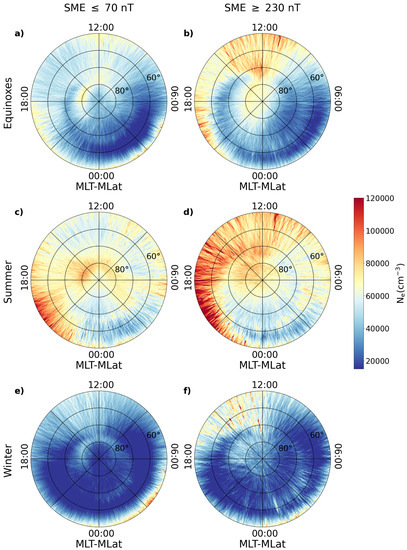
Figure 1.
Polar view of the average spatial distribution of electron density () for low (a,c,e) and high (b,d,f) geomagnetic activity conditions in the Northern Hemisphere as represented in the QD–magnetic latitude (MLat) and MLT reference system. Each column shows the average spatial distribution of electron density during three different periods of the year: equinoxes, summer, and winter. The maps are based on data collected by the Swarm A satellite from 1 January 2016 to 31 December 2021, and reflect an average altitude of approximately 460 km. The concentric circles are plotted in intervals, with the outermost circle corresponding to .
3. Method: EMD and its Multivariate Extension
Empirical Mode Decomposition (EMD) is a data analysis technique first introduced by Huang et al. [23] with the aim of adaptively representing non-stationary signals. The fundamental concept is that a signal can be decomposed in a finite, often small number of intrinsic oscillatory modes, each one of them reproducing the repeating behaviour of the signal at a specific time scale [24]. The EMD method allows signals that are not compatible with the Fourier Transform restrictions to be analyzed. In fact, Fourier analysis is a powerful method of extracting the energy–frequency distribution of a signal, and is widely used for its simplicity and its general applicability; however, it cannot produce physically meaningful results when dealing with nonstationary data [23]. In such cases, EMD can resolve the role of reducing the signal into a set of basis signals
which are derived directly from the data itself [24].
The empirical modes must fulfill two criteria: first, when considering the entire dataset, each of these function must have the same number of extrema (local maxima and/or minima) and zero crossings or differ by one at most; second, when considering any point, the mean value between the envelopes defined by the local maximum and local minimum must be zero [23]. The resulting functions are simple oscillatory modes, which differ from simple harmonic components in that their frequency and amplitude can change along the time frame.
The procedure for extracting the empirical modes, called sifting, involves the following steps:
- The local extrema of the considered dataset are identified.
- A cubic spline is used to connect all the local maxima in order to obtain the upper envelope.
- Another cubic spline is used to connect all the local minima in order to obtain the lower envelope.
- The mean between the two envelopes () is computed.
- The first component is obtained by subtracting from the data .
- If is a function with zero mean, it is accepted as the first empirical mode, ; otherwise, undergoes steps 1–5 itself and the procedure is repeated until fulfills the zero mean criterion.
In addition, it is necessary to apply a stopping criteria to the number of sifting iterations; in this way, the obtained empirical modes preserve the amplitude and frequency modulation as well as their physical sense [23]. One potential stopping criterion is to determine a threshold limit for the size of the standard deviation between two consecutive sifting steps k and :
in which is usually fixed at 0.3 [23]. To obtain the following empirical modes, the process is successively applied to the residual . The procedure described above is then repeated until the residual becomes a constant, a monotonic function, or a function with only one maximum and minimum from which it is not possible to extract other modes [24]. If necessary, it is then possible to compute the instantaneous frequencies and amplitudes of each obtained mode by applying the Hilbert transform to each of the modes. When adding this final step, the full process is called the Hilbert–Huang Transform [24].
In the presence of multivariate signals, the definition of local extrema becomes more complicated, making the step of local mean estimation non-obvious [25]. Therefore, in these cases it is not possible to apply directly EMD, and becomes necessary to employ its multivariate extension (MEMD). After the first proposals of EMD extension to complex/bivariate [26,27] and trivariate data [28], Rehman and Mandic [25] proposed a way of extending the concept of local extrema to an N-dimensional space. The N-variate signal has to be subdivided into N-dimensional datasets, each of which is then projected along different directions in the N-dimensional space. Each projected signal has its own envelopes for each of the directions, and the local mean can be computed by averaging over the N-dimensional space. The local mean can be computed through two different methods, both involving the selection of a suitable set of direction vectors in the N-dimensional space. In the first method, uniform angular sampling of a unit sphere in an N-dimensional hyperspherical coordinate system is used to obtain a set of direction vectors that covers the whole () sphere. The second method is based on low-discrepancy point sets, in which discrepancy refers to a quantitative measure of the irregularity or non-uniformity of a distribution. This approach belongs to the class of quasi-Monte Carlo methods [29]. Through either methods, a uniform distribution of direction vectors is obtained that can provide more accurate estimation of the local mean in N-dimensional spaces. Multivariate empirical modes can be successively obtained following the already mentioned procedure of standard EMD by using multivariate spline interpolation and checking the obtained modes properties [30]. An important difference with EMD is that in MEMD the condition of equality between the numbers of extrema and zero crossings is not imposed, as the definition of extrema is not straightforward for multivariate signals [31].
In this work, we used a Python algorithm to apply the MEMD method, available at https://github.com/mariogrune/MEMD-Python-, accessed on 20 April 2023; it is an adaptation of the procedure described in Rehman and Mandic [25] and is produced in Matlab (freely available at: http://www.commsp.ee.ic.ac.uk/~mandic/research/emd.htm). We chose to use this Python version because of its applicability to input data characterized by any number of channels. In fact, as an input for this MEMD algorithm we utilized the two-dimensional matrix obtained by binning the electron density data into a grid of 1× 1 in magnetic latitude and MLT, where 1 corresponds to 4 min in MLT. Each bin in the map reports the mean electron density value considering all the Swarm measurements that fall within it. Here, we are interested in the region above 50 in magnetic latitude; in order to avoid a bad description of the lower latitude border, however, we obtained a map above 45. On the other hand, to account for the cylindrical symmetry in MLT, where the values of the first column in MLT (MLT = 00:00) must be the same as those of the last column in MLT (MLT = 24:00), we extended the matrix by replicating the original matrix three times. In this way, the input matrix has a dimension of 45× 1080. Thus, the MEMD algorithm returns (N + 1) matrices 45× 1080, representing the N modes plus the residue in which the signal is decomposed. From each of these N matrices, we selected the 360 central columns and the rows representing the latitudes above 50. In this way, (N + 1) rectangular maps of 40× 360 are obtained, represented in polar coordinates, allowing for better visualization of the spatial distributions of the features characterizing each mode.
Each multivariate empirical mode is characterized by a distinctive scale, which can be roughly visualized by considering a fixed magnetic latitude and checking how many times the electron density passes from positive to negative values. This happens with a specific periodicity in MLT depending on the mode. We evaluated this average timescale/period by considering the 40 time series of 360 data points, obtainable from each one of the 40 rows of the aforementioned matrix. It is possible to obtain a periodogram from each series that provides the signal spectral density as a function of the frequency. By averaging the 40 periodograms relative to each fixed magnetic latitude, a single mean periodogram characterized by a peak corresponding to the most significant frequency of the mode can be obtained. The inverse of the frequency corresponding to this Fourier PSD peak provides an indication of the longitudinal variability associated with the considered mode. Because we report our results in MLT coordinates, we are able to represent the average periods in units of time (minutes).
4. Results
We begin our investigation by applying the MEMD method to the electron density distribution during the equinox period when geomagnetic activity is low. Figure 2 presents the results of the decomposition. We obtained a total of eight modes plus the residue. These are represented on polar maps by plotting their average electron density value using QD latitude and MLT. The top of the map corresponds to noon and the bottom to midnight; the MLT equal to 06:00 (on the right) and 18:00 (on the left) is indicated in order to better visualize the morning and evening sectors, and a 1× 1 binning grid is used.
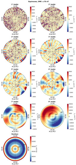
Figure 2.
Polar view of the eight modes and the residue obtained from the MEMD of electron density distribution during the equinoctial period, in the Northern Hemisphere, when geomagnetic activity is low. Maps are represented using the QD–magnetic latitude (MLat) and MLT reference system. The concentric circles are plotted in intervals, with the outermost circle corresponding to .
In Figure 3, the left side shows the average period obtained through the latitudinal averaged frequency analysis associated with each mode and right side shows the energy distribution in terms of the normalized variance of each mode with respect to the total variance of the signal. Observing the energy trend of each mode, the first six exhibit extremely low energy levels, with a normalized variance value lower than that of the first mode; as a result, because the EMD acts as a dyadic filter [32] and the first mode is usually associated with the noise content of the signals [33], when the normalized variance is less than that of the first mode it cannot be physically meaningful in the statistical sense.
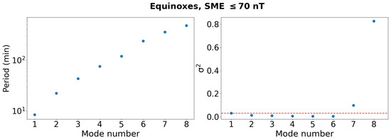
As a result of analyzing the energy contribution of each mode to the original signal, it is clear that the last two modes and the residue contribute significantly to the description of the initial distribution. By examining the time periods associated with each mode, however, three distinct trends emerge, allowing the obtained modes to be classified into three classes. The first class includes the first two modes, the second class includes the four following modes (from the third to the sixth mode), and the third class includes the seventh and eighth modes.
We examined any variations with the latitude in the average period value for each of these four modes by conducting a comprehensive analysis of the periodicities of the modes in MLT belonging to the second class. The periodogram for a given magnetic latitude value was computed by taking into account the series of density values corresponding to different MLTs. This entailed analyzing 40 distinct periodograms for each mode obtained from a series of 360 data points, with a resolution of 1 for both magnetic latitude and MLT. The fundamental frequency value was calculated from each periodogram based on the peak position. The average period was then calculated using the frequency values in MLT, with the period found to be practically constant with the latitude for all four analyzed modes. The average periods obtained for each one of the four modes are (), (), (), and () min. These periodicities are in good agreement with the harmonics and subharmonics of the satellite’s orbital period (∼94 min). In other words, the spatial structure of the electron density distribution associated with these modes closely resembles the satellite traces, implying a possible link to the data acquisition process. However, we note that these modes do not contribute significantly to the overall decomposition, because their energy remains lower than that of the first one. As a result, we combine this second class of modes together and consider a smaller number of modes for further analysis.
Figure 4 illustrates the grouped modes that effectively describe the fundamental modes present in the spatial distribution of electron density in the Northern Hemisphere. The modes (labeled hereinafter by Roman numerical notation) and the residue are among them. The first mode (I mode), which is essentially noise, is the sum of the initial two modes. The second mode (II mode), a combination of the third to sixth initial modes, is associated with the satellite’s orbit. The third (III) and fourth (IV) modes are direct results of the initial decomposition, and given their higher energy values represent the primary modes through which the original signal is decomposed.
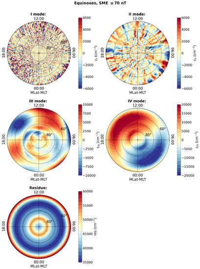
Figure 4.
Polar view of the fundamental modes and residue obtained from the Multivariate Empirical Mode Decomposition (MEMD) of electron density distribution during the equinoctial period under low geomagnetic activity in the Northern Hemisphere. Imode corresponds to the sum of the and modes reported in Figure 2, II mode corresponds to the sum of the , , , and modes in Figure 2, and III and IV modes are equal to the and modes in Figure 2, respectively. Maps are represented in the QD–magnetic latitude (MLat) and MLT reference system. The concentric circles are plotted in intervals, with the outermost circle corresponding to .
The same identical procedure was used for the electron density distributions during summer and winter seasons when the geomagnetic activity was low, and was repeated for the geomagnetically disturbed period. In all the analyzed cases, regardless of the season and the geomagnetic activity level, the original electron density distribution is consistently decomposed into eight modes along with the residue. In addition, during all the analyzed configuration, which are not shown here for brevity, the modes’ average periods and energy distributions follow the same behaviour as the one obtained in the first study case, i.e., during the equinoctial period and low geomagnetic activity, as reported in Figure 3. This makes it clear that even in the other five configurations under analysis it was possible to distinguish three different classes of modes which contribute different amounts of energy to the original signal. This observation led us to use the same mode grouping approach described in detail previously during the equinoctial period of low geomagnetic activity. In this way, in each case we obtained four decomposed modes accompanied by their residue. The third and fourth modes and the residue obtained for each configuration of season and geomagnetic activity level are the ones that provide the more relevant contributions to the electron density description, and are shown and discussed in the following Section 5.
5. Discussion
Application of the MEMD method to the spatiotemporal distribution of electron density at middle and high latitudes in the Northern Hemisphere under various seasonal and geomagnetic activity conditions reveals the presence of fundamental modes that underlie the initial distributions. Surprisingly, these modes are consistently observed in all six datasets regardless of the specific season or level of geomagnetic activity under consideration. Each electron density dataset can be accurately reconstructed by combining the residue with these four distinct fundamental modes.
To gain a better understanding of the physical processes associated with each mode, we examine its spatiotemporal distribution and how it varies across seasons and levels of geomagnetic activity. We begin with the residue term, which is the basis of the electron density distribution and to which the modes are later added to reconstruct the initial distribution. We find a striking similarity in the spatiotemporal structure of the residues obtained under low geomagnetic activity across the three seasonal periods, as can be seen in the left column of the upper part of Figure 5. The electron density is highest at lower latitudes and gradually decreases towards higher latitudes, reaching a minimum around 60–65. It then begins to rise again, reaching a peak near 80 before falling near the magnetic pole. This pattern reveals two distinct bands of maximum intensity, one below 55 magnetic latitude and another between 75 and 85 magnetic latitudes. Lower electron density regions exist primarily between 55 and 75 latitudes and near the magnetic pole, corresponding to the polar cap. While the spatiotemporal position of these bands remains consistent across seasons, the absolute values of the electron density and intensity ratios between the different bands change.
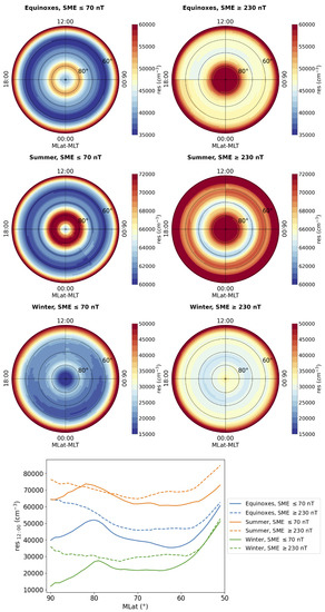
Figure 5.
(Upper part): polar view of residue obtained from the MEMD of electron density distribution during the equinoxes (first row), summer (second row), and winter (third row) under low (left column) and high (right column) geomagnetic activity conditions in the Northern Hemisphere. Maps are represented in the QD–magnetic latitude (MLat) and MLT reference system. The concentric circles are plotted in intervals, with the outermost circle corresponding to . (Bottom part): residue trend as a function of the magnetic latitude at a fixed MLT value of 12:00 for the three seasons and two levels of geomagnetic activity.
The upper part of Figure 5 depicts the spatiotemporal distributions of residues, which cannot be effectively represented using a single value scale in all cases. Therefore, to better compare the different configurations using a common scale, the bottom part of Figure 5 displays various electron density profiles as a function of the magnetic latitude for the studied season and level of geomagnetic activity in a single graph. This provides a comprehensive view of the spatial variations in electron density across different latitudes, enabling a detailed examination of the patterns and changes associated with each specific season and level of geomagnetic activity. These profiles correspond to a fixed MLT = 12:00, and clearly show that the electron density is higher during summer than during winter at all latitudes and exceeds the density observed during the equinoxes. This consistent pattern holds regardless of geomagnetic activity. The variation in the baseline electron density, which varies depending on the time period under study, corresponds to the differences observed in the distribution of electron density in the F-layer of the ionosphere between seasons (summer, winter, and equinoxes). When compared to other seasons, the summer has a higher electron density. This is due to an increase in solar radiation, which heats both the atmosphere and the ionosphere. Elevated temperatures promote the ionization of atoms and molecules, resulting in a higher electron density in the F-layer of the ionosphere. This effect is particularly pronounced in the equatorial and lower-latitude regions, where solar radiation is stronger. However, as our research shows, similar phenomena can be observed at higher latitudes as well. Winter, on the other hand, sees a decrease in electron density in the F-layer of the ionosphere. Solar radiation is less intense during this season, and the atmospheric and ionospheric temperatures are generally lower. As a result, there is less ionization of atoms and molecules in the atmosphere, resulting in a lower electron density in the F-layer of the ionosphere. The decrease in electron density is most noticeable in the polar regions, where solar radiation is scarce or non-existent during the winter months. There is an intermediate distribution of electron density in the ionosphere’s F-layer during the equinoxes, which mark the transition between summer and winter. When compared to other seasons, the moderate solar radiation and temperatures during these times result in a relatively balanced electron density. Therefore, the spatiotemporal pattern of the residues reflects the fluctuations in electron density within the F-layer of the ionosphere throughout the seasons which arise from the complex interplay between solar radiation, atmospheric temperatures, and ionization processes.
The seasonal differences in the spatiotemporal distributions of the residues obtained by decomposing the electron density distributions remain visible during periods of high geomagnetic activity. The spatial and temporal distribution of the electron density within the residue is higher during the summer compared to the winter and equinox seasons. Figure 5 reveals that the average level of electron density is affected by both the season and the level of geomagnetic activity, with notable changes occurring during periods of high geomagnetic activity. The minimum in the density distribution within the polar cap region vanishes, replaced by a single region of maximum electron density spanning the entire polar region that begins around 80. Additionally, the band of the minimum electron density shifts towards higher latitudes. The residue maps exhibit a minimum region around 75, with a subsequent displacement towards the polar region of approximately 5 compared to the quiet condition. The finding that an increase in geomagnetic activity causes an increase in electron density in the F region of the ionosphere is consistent with previous research. This increase in average electron density can be attributed to a number of well-studied and documented factors. One factor is the enhanced energy input from the magnetosphere during periods of geomagnetic activity. Geomagnetic disturbances such as substorms and magnetic storms can lead to the injection of energetic particles into the ionosphere. These particles ionize the neutral particles in the F region, resulting in an increase in electron density. Another factor is the enhancement of electric fields and plasma convection associated with geomagnetic activity. Electric fields generated by the interaction between the solar wind and the Earth’s magnetosphere can accelerate charged particles in the ionosphere, leading to increased electron density. Driven by the motion of plasma within the magnetosphere, plasma convection can transport higher-density plasma in the ionosphere from lower latitudes to higher latitudes. Furthermore, increased geomagnetic activity can lead to changes in thermospheric composition and temperature. These changes can affect the ionization and recombination rates in the F region, influencing the electron density. It is important to note that the relationship between geomagnetic activity and electron density in the F region is complex, and varies depending on the circumstances and location. It is worth noting, however, that the residues obtained from our analysis appear to capture these changes, providing insights into the variations in electron density associated with geomagnetic activity.
We now examine the four modes resulting from each decomposition. The first of these modes, reported only for the equinoctial and low geomagnetic activity case in Figure 4, is analogous to the other five configurations (data not shown), and essentially represents a noise component present in the data. Starting from an analysis of the data distribution resulting from an average, this term could be due to small-scale variations in the original distribution. However, the energy associated with this mode is extremely low, and there are no significant structures in its distribution on the MLat–MLT plane. On the other hand, the second mode (for brevity, data are shown only for the equinoctial and low geomagnetic activity configuration in Figure 4) is quite different. As extensively discussed in the previous section, this mode exhibits a spatial structure that closely resembles the orbit of the satellite from which the data were acquired. The average frequency of this mode is consistent across latitudes, and is comparable to the orbital period of the satellite around the Earth. Finally, the third and fourth modes capture our interest because they are intricately linked to dynamic processes occurring within the ionospheric layer under investigation. These modes exhibit a strong dependence on both the season and the level of geomagnetic activity, making them particularly intriguing and worthy of further exploration.
To gain insight into the dynamic processes that contribute to the distribution of electron density for these two modes regardless of season or activity level, convection cell structures are overlaid onto the maps depicting these modes. At high latitudes, the ionized region of the upper atmosphere undergoes a dynamic circulation known as convection driven by the interaction of the magnetized solar wind and the Earth’s magnetosphere. This convection is important in determining the distribution of electron density in the ionosphere. The convection patterns are twin-celled in nature, with the flow moving away from the Sun at the poles and toward the Sun at lower latitudes. The strength of this circulation is influenced by the north–south component of the IMF (represented as ), while any asymmetries between the dawn and dusk regions are associated with the east–west component of the IMF (). In general, convection exhibits a highly dynamic nature, displaying sensitivity to intermittent phenomena such as variations in the IMF and magnetospheric processes such as substorms. One effective method for capturing and analyzing these convection patterns is to utilize data from the Super Dual Auroral Radar Network (SuperDARN). SuperDARN is a widespread network of scientific radars designed to monitor the near-Earth space environment. Each radar within the network is capable of measuring the velocity of ionospheric plasma. By combining data from multiple radars, a comprehensive view of plasma motion in the polar ionosphere can be obtained, enabling studies on the electromagnetic interaction between the solar wind and Earth’s magnetosphere [34]. Using a long period of SuperDARN data, a dynamic model of convection can be constructed to enable the precise determination of the electrostatic potential distribution in high latitude regions for a wide range of solar wind, IMF, and dipole tilt parameter values [35]. In our case, we obtained representative average convection motions that reflect the interplanetary conditions underlying the originated data by calculating the mean values of the x-component of the solar wind velocity (), the y- and z-components of the magnetic field, and the dipole tilt for each of the six different datasets analyzed and presented in Figure 1. The obtained values, which refer to the time intervals used to build the different datasets, were then incorporated into the CS10 model [36], enabling us to obtain the average trends of the electrostatic potential distribution. Table 1 reports the values of the solar wind velocity, the two components of the magnetic field, and the dipole tilt used in the different cases. Figure 6 illustrates the spatial and temporal distributions of the electron density for the third and fourth fundamental modes obtained from decomposition during low geomagnetic activity. The figure consists of six maps, with each pair representing the III and IV modes for the analyzed equinoctial, summer, and winter periods. Each map includes the average electrostatic potential level curves overlaid on top of the electron density spatiotemporal distribution. Similarly, Figure 7 follows the same structure as Figure 6 with a focus on the period of high geomagnetic activity.

Table 1.
Interplanetary parameters and dipole tilts used as input values for the SuperDARN model relative to each one of the seasonal and geomagnetic activity conditions considered in the present study.
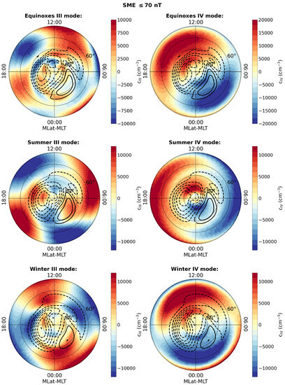
Figure 6.
Polar view of the III and IV fundamental modes obtained from the MEMD of electron density distribution during the equinoctial (first row), summer (second row), and winter (third row) periods under low geomagnetic activity in the Northern Hemisphere. SuperDARN polar potential maps obtained using the statistical convection model CS10 are superimposed on each mode as level curves. Maps are represented in the QD–magnetic latitude (MLat) and MLT reference system. The concentric circles are plotted in intervals, with the outermost circle corresponding to .
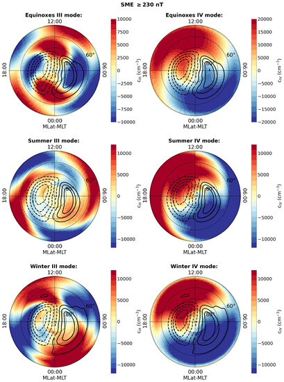
Figure 7.
Polar view of the III and IV fundamental modes obtained from the MEMD of electron density distribution during the equinoctial (first row), summer (second row), and winter (third row) periods under high geomagnetic activity in the Northern Hemisphere. SuperDARN polar potential maps obtained using the statistical convection model CS10 are superimposed on each mode as level curves. Maps are represented in the QD–magnetic latitude (MLat) and MLT reference system. The concentric circles are plotted in intervals, with the outermost circle corresponding to .
We begin with the fourth mode and its relationship to the season and geomagnetic activity, as well as the structure of the convection cells superimposed on each map. Here, we are specifically looking at all of the electron density maps shown in the right column of Figure 6 and Figure 7. The electron density spatiotemporal distribution exhibits a clear day–night difference. The spatiotemporal distribution during equinoxes shows higher density values within the MLT interval between 7:00 and 20:00, with a peak occurring between 11:00 and 18:00. This pattern is consistent across all studied latitudes. This day–night asymmetry is primarily attributed to the interaction between solar radiation and the Earth’s atmosphere. During the day, solar radiation provides a significant amount of energy that ionizes the upper atmosphere, resulting in higher electron density in the F-layer. Conversely, during the night solar radiation is absent or significantly reduced, leading to a decrease in ionization and electron production. Another contributing factor to the day–night asymmetry is the recombination effect that takes place during the night. Without direct solar radiation, electrons in the ionospheric plasma tend to recombine with ions, leading to a decrease in electron density within the F-layer throughout the nighttime. Furthermore, ionospheric wind movements and diffusion processes can influence electron distribution, adding to the day–night asymmetry. These factors contribute to the creation of plasma flows that shift electron density across different regions of the ionosphere during various phases of the day and night. It is interesting to note that there is a difference in the day–night asymmetry of the electron distribution between the summer and winter seasons. During the summer there is generally higher ionization of the upper atmosphere due to more direct and prolonged solar incidence, resulting in a higher electron density in the F-region during daylight hours. As a result, the amplitude of the day–night asymmetry may be greater in the summer than in the winter. This is precisely what is observed when comparing the results obtained for this fourth mode in summer and winter. However, it is important to note that the day–night asymmetry depends on other factors as well, such as the latitude, solar activity, and presence of geomagnetic events. In this study, we fixed the level of solar activity while analyzing two levels of geomagnetic activity. When examining the characteristics of the fourth mode during high geomagnetic activity across different seasons, as shown in the maps in the right column of Figure 7, it can be seen that the day–night asymmetry follows the same seasonal patterns, with only the intensity level varying. Overall, it can be concluded that the fourth mode, obtained through the decomposition of the different datasets, is the result of a combination of factors including interaction with the solar radiation, the nighttime electron recombination process, and ionospheric wind movements. These processes play a dominant role compared to the other modes, as the fourth mode is the most energetic one.
While the analysis of the convection cell structure makes no significant contribution to a better understanding of the electron density distribution in the fourth mode, it is critical to comprehending the third mode. The third mode is presented in Figure 6 and Figure 7 (left columns) in relation to the season and the level of geomagnetic activity. During periods of high geomagnetic activity, the third mode exhibits a region of high electron density at high latitudes on the day side. This characteristic is consistent throughout the year. This region corresponds to the cusp, which is a distinct area within the day side auroral oval near noon. The cusp is known for enhanced ion and electron precipitation, and is considered the primary location for the transport of magnetosheath plasma into the ionosphere. It typically appears as a single spot that spans a few hours of MLT, and its position is influenced by the and components of the IMF. However, it is important to note that the cusp does not always manifest as a single structure. In certain cases, especially when the IMF component is large or when there are changes in IMF orientation, the cusp can bifurcate into two or more distinct regions. This bifurcation phenomenon adds complexity to the cusp structure, and highlights the dynamic nature of the interaction between the solar wind and Earth’s magnetosphere. During periods of high geomagnetic activity, various phenomena contribute to the dynamic nature of the high-latitude mesoscale ionosphere. Precipitating electrons propagate towards the pole, and localized structures of electron density known as polar cap patches can be observed moving into and across the polar cap region; additionally, flux transfer events (FTEs) occur, in which photoionized plasma from closed field lines on the day side is transported into the polar cap across the boundary between open and closed field lines. These processes lead to plasma redistribution and changes in plasma density structures in the surrounding regions. The third mode effectively captures the overall results of electron motion, showing an evident increase in electron density along the two convection cells in the polar cap region and subsequent accumulation on the night side at high latitudes. The outcome of this dynamic is significantly less pronounced during periods of low geomagnetic activity, likely due to the influence of a predominantly positive IMF z-component (see Table 1), which affects the configuration of the convection cells, as well as to lower overall dynamics in this region compared to the geomagnetic disturbance period.
6. Summary and Conclusions
For the first time, the MEMD method was used to examine the spatiotemporal distribution of ionospheric electron density at middle and high latitudes (above magnetic latitude) in the Northern Hemisphere as recorded by the Swarm satellite constellation between 1 January 2016, and 31 December 2021. In this research, we looked at different levels of seasonal and geomagnetic activity and discovered the fundamental modes that underpin the initial distributions. By combining these modes with the residue, we were able to precisely reconstruct each electron density dataset. Interestingly, the same number of modes were consistently observed in all datasets regardless of season or geomagnetic activity. Typically, the number of extracted modes is dependent on factors such as the number of datapoints, the presence of different noise sources, and/or additional short-term contributions. In our case, we expect that the noise is the same for the different seasons, and we have the same number of points; thus, these two aspects should not change the number of modes and only differences in short-term variability between the quiet and disturbed period can change the number of modes. Because this does not occur, ew can conclude that similar scale-dependent processes form the basis of the different spatiotemporal patterns seen across different seasons and geomagnetic conditions.
We were able to identify four distinct modes: the first mode represents noise or small-scale variations; the second is characterized by a constant frequency across latitudes, similar to the satellite’s orbit; and seasonality and geomagnetic activity dependence are observed in the third and fourth modes, which are linked to dynamic processes within the ionospheric layer. According to our findings, the third mode describes the dynamic processes in high-latitude ionospheric circulation, which is typical of the polar cap region, while the fourth mode emphasizes day–night differences caused by solar radiation, recombination, and ionospheric wind movements. The four modes do not contribute to the original signal in the same way; the most important are the last two modes, which are the most energetic. All of these modes must be added to a base, which is the residue, in order to reconstruct the initial electron density distribution. The residue is higher in the summer than in the winter at all latitudes, and exceeds the density observed during the equinoxes. This consistent pattern persists regardless of geomagnetic activity, though as geomagnetic activity increases the average value of the electron density increases for all latitudes and MLTs.
It is critical to emphasize that our results accurately depict the ionospheric dynamics at both middle and high latitudes during a quiet solar period. It is known that solar activity has a significant impact on the ionosphere, indicating the need to replicate this analysis using years with increased solar activity to confirm our findings’ ongoing relevance or detect any potential changes. In general, we anticipate that the decomposition should remain mostly unchanged, though the relative importance of each mode may shift. With the onset of a period of increased solar activity and the continued operation of the Swarm satellite constellation in orbit, we expect to soon be able to investigate the relationship between the solar cycle and the results obtained in this paper.
In conclusion, our research has revealed important insights into the spatiotemporal distribution of the electron density, thereby advancing our understanding of the ionosphere and its spatiotemporal variations while allowing us to better understand its complex behavior. These findings carry relevance for ionospheric models, offering the ability to pinpoint spatiotemporal electron density distributions tied to distinct dynamic processes within the studied ionospheric area. Additionally, they provide insights into the energy contributions of these processes. By integrating these spatiotemporal distributions and energy factors into models, a more precise and comprehensive depiction of the ionosphere could be achieved. In turn, this advance could lead to more accurate prediction of forthcoming ionospheric conditions. Indeed, these findings could be similarly applied to the recent development of a prediction model of Total Electron Content (TEC) derived from GPS data [37]. In this case, a hybrid approach combining Ensemble Empirical Mode Decomposition (EEMD) and Long Short-Term Memory (LSTM) deep learning was utilized. Similarly, one could consider applying the obtained results by directly employing machine learning techniques, as recently proposed by [38], to construct a global model for TEC using Global Ionospheric Maps data along with features such as geomagnetic and solar activity indexes.
Author Contributions
Conceptualization, P.D.M. and T.A.; methodology, G.L. and T.A.; formal analysis, G.L.; investigation, P.D.M., G.L., T.A. and G.C.; data curation, G.L.; writing—original draft preparation, P.D.M. and G.L.; writing—review and editing, all authors. All authors have read and agreed to the published version of the manuscript.
Funding
T.A. received funding from the “Bando per il finanziamento di progetti di Ricerca Fondamentale 2022” mini-grant of the Italian National Institute for Astrophysics (INAF) for “The predictable chaos of space weather events”.
Data Availability Statement
Swarm satellite data can be accessed at http://earth.esa.int/swarm, accessed on 15 January 2022. SuperMAG data are available at https://supermag.jhuapl.edu/, accessed on 18 April 2023. IMF components and solar wind speed data are freely available at https://cdaweb.gsfc.nasa.gov/index.html/, accessed on 2 November 2022.
Acknowledgments
The results presented herein rely on data collected by the ESA’s Swarm mission. We thank the European Space Agency that supports the Swarm mission. We gratefully acknowledge the SuperMAG collaborators (https://supermag.jhuapl.edu/info/?page=acknowledgement, accessed on 18 April 2023). The IMF components and solar wind velocity data were obtained from the OMNIWeb Data Explorer website, which is operated by the Goddard Space Flight Center (NASA) Space Physics Data Facility, for which we are grateful. In addition, we acknowledge the national scientific funding agencies of Australia, Canada, China, France, Italy, Japan, South Africa, UK, and USA that funded the SuperDARN radar network. G.L. acknowledges the PhD course in Astronomy, Astrophysics, and Space Science of the University of Rome “Sapienza”, University of Rome “Tor Vergata”, and Istituto Nazionale di Geofisica e Vulcanologia, Italy.
Conflicts of Interest
The authors declare no conflict of interest.
Abbreviations
The following abbreviations are used in this manuscript:
| ACC | Accelerometer |
| AE | Auroral Electrojet |
| ASM | Absolute Scalar Magnetometer |
| EFI | Electric Field Instrument |
| EEMD | Ensamble Empirical Mode Decomposition |
| EMD | Empirical Mode Decomposition |
| ESA | European Space Agency |
| EO | Earth Observation |
| EUV | Extreme Ultra Violet |
| FTE | Flux Transfer Event |
| GLONASS | Globalnaya Navigazionnaya Sputnikovaya Sistema |
| GNSS | Global Navigation Satellite System |
| GPS | Global Positioning System |
| GPSR | GPS Receiver |
| IMF | Interplanetary Magnetic Field |
| LP | Langmuir Probe |
| LRR | Laser Retro-Reflector |
| LSTM | Long Short-Term Memory |
| MEMD | Multivariate Empirical Mode Decomposition |
| MIT | Main Ionospheric Trough |
| MLT | Magnetic Local Time |
| QD | Quasi-Dipole |
| SED | Storm-Enhanced Density |
| STR | Star Tracker |
| SuperDARN | Super Dual Auroral Radar Network |
| TEC | Total Electron Content |
| TII | Thermal Ion Imager |
| VFM | Vector Field Magnetometer |
References
- Kelly, M.C. The Earth’s Ionosphere: Plasma Physics and Electrodynamics, 2nd ed.; Elsevier: Amsterdam, The Netherlands, 2009. [Google Scholar]
- Klobuchar, J.A. Ionospheric time-delay algorithm for single-frequency GPS users. IEEE Trans. Aerosp. Electron. Syst. 1987, AES-23, 325–331. [Google Scholar] [CrossRef]
- Prieto-Cerdeira, R.; Orús-Pérez, R.; Breeuwer, E.; Lucas-Rodriguez, R.; Falcone, M. Performance of the Galileo single-frequency ionospheric correction during in-orbit validation. GPS World 2014, 25, 53–58. [Google Scholar]
- Yuan, Y.; Wang, N.; Li, Z.; Huo, X. The BeiDou global broadcast ionospheric delay correction model (BDGIM) and its preliminary performance evaluation results. Navigation 2019, 66, 55–69. [Google Scholar] [CrossRef]
- Friis-Christensen, E.; Lühr, H.; Hulot, G. Swarm: A constellation to study the Earth’s magnetic field. Earth Planets Space 2006, 58, 351–358. [Google Scholar] [CrossRef]
- Milan, S.E.; Grocott, A. High Latitude Ionospheric Convection. In Ionosphere Dynamics and Applications; Huang, C., Lu, G., Eds.; AGU: Hoboken, NJ, USA, 2021; Volume 3, p. 21. [Google Scholar] [CrossRef]
- Cowley, S.W.H. TUTORIAL: Magnetosphere-Ionosphere Interactions: A Tutorial Review. Geophys. Monogr. Ser. 2000, 118, 91. [Google Scholar] [CrossRef]
- Prölss, G.W.; Bird, M.K. Physics of the Earth’s Space Environment: An Introduction; Springer: Berlin/Heidelberg, Germany, 2004. [Google Scholar]
- Tashchilin, A.; Romanova, E. Numerical modeling the high-latitude ionosphere. In Proceedings of the Solar-Terrestrial Magnetic Activity and Space Environment: Proc. COSPAR Colloquium, Beijing, China, 10–12 September 2001; Volume 14. [Google Scholar]
- Fratter, I.; Léger, J.M.; Bertrand, F.; Jager, T.; Hulot, G.; Brocco, L.; Vigneron, P. Swarm Absolute Scalar Magnetometers first in-orbit results. Acta Astronaut. 2016, 121, 76–87. [Google Scholar] [CrossRef]
- Knudsen, D.J.; Burchill, J.K.; Buchert, S.C.; Eriksson, A.I.; Gill, R.; Wahlund, J.E.; Åhlen, L.; Smith, M.; Moffat, B. Thermal ion imagers and Langmuir probes in the Swarm electric field instruments. J. Geophys. Res. Space Phys. 2017, 122, 2655–2673. [Google Scholar] [CrossRef]
- Buchert, S.; Zangerl, F.; Sust, M.; André, M.; Eriksson, A.; Wahlund, J.E.; Opgenoorth, H. SWARM observations of equatorial electron densities and topside GPS track losses. Geophys. Res. Lett. 2015, 42, 2088–2092. [Google Scholar] [CrossRef]
- Xiong, C.; Stolle, C.; Park, J. Climatology of GPS signal loss observed by Swarm satellites. Ann. Geophys. 2018, 36, 679–693. [Google Scholar] [CrossRef]
- Visser, P.; Doornbos, E.; van den IJssel, J.; Teixeira da Encarnação, J. Thermospheric density and wind retrieval from Swarm observations. Earth Planets Space 2013, 65, 1319–1331. [Google Scholar] [CrossRef]
- Gjerloev, J.W. The SuperMAG data processing technique. J. Geophys. Res. (Space Phys.) 2012, 117, A09213. [Google Scholar] [CrossRef]
- Newell, P.T.; Gjerloev, J.W. Evaluation of SuperMAG auroral electrojet indices as indicators of substorms and auroral power. J. Geophys. Res. (Space Phys.) 2011, 116, A12211. [Google Scholar] [CrossRef]
- Davis, T.N.; Sugiura, M. Auroral electrojet activity index AE and its universal time variations. J. Geophys. Res. (1896–1977) 1966, 71, 785–801. [Google Scholar] [CrossRef]
- Bergin, A.; Chapman, S.C.; Gjerloev, J.W. AE, DST, and Their SuperMAG Counterparts: The Effect of Improved Spatial Resolution in Geomagnetic Indices. J. Geophys. Res. (Space Phys.) 2020, 125, e27828. [Google Scholar] [CrossRef]
- Richmond, A.D. Ionospheric Electrodynamics Using Magnetic Apex Coordinates. J. Geomagn. Geoelectr. 1995, 47, 191–212. [Google Scholar] [CrossRef]
- Rodger, A.S.; Moffett, R.J.; Quegan, S. The role of ion drift in the formation of ionisation troughs in the mid- and high-latitude ionosphere—A review. J. Atmos. Terr. Phys. 1992, 54, 1–30. [Google Scholar] [CrossRef]
- Zou, S.; Moldwin, M.B.; Ridley, A.J.; Nicolls, M.J.; Coster, A.J.; Thomas, E.G.; Ruohoniemi, J.M. On the generation/decay of the storm-enhanced density plumes: Role of the convection flow and field-aligned ion flow. J. Geophys. Res. (Space Phys.) 2014, 119, 8543–8559. [Google Scholar] [CrossRef]
- Foster, J.C.; Erickson, P.J.; Coster, A.J.; Goldstein, J.; Rich, F.J. Ionospheric signatures of plasmaspheric tails. Geophys. Res. Lett. 2002, 29, 1623. [Google Scholar] [CrossRef]
- Huang, N.E.; Shen, Z.; Long, S.R.; Wu, M.C.; Shih, H.H.; Zheng, Q.; Yen, N.C.; Tung, C.C.; Liu, H.H. The empirical mode decomposition and the Hilbert spectrum for nonlinear and non-stationary time series analysis. Proc. R. Soc. London. Ser. A Math. Phys. Eng. Sci. 1998, 454, 903–995. [Google Scholar] [CrossRef]
- Maheshwari, S.; Kumar, A. Empirical mode decomposition: Theory & applications. Int. J. Electron. Eng. 2014, 7, 873–878. [Google Scholar]
- Rehman, N.; Mandic, D.P. Multivariate empirical mode decomposition. Proc. R. Soc. A Math. Phys. Eng. Sci. 2010, 466, 1291–1302. [Google Scholar] [CrossRef]
- Tanaka, T.; Mandic, D.P. Complex empirical mode decomposition. IEEE Signal Process. Lett. 2007, 14, 101–104. [Google Scholar] [CrossRef]
- Altaf, M.U.B.; Gautama, T.; Tanaka, T.; Mandic, D.P. Rotation invariant complex empirical mode decomposition. In Proceedings of the 2007 IEEE International Conference on Acoustics, Speech and Signal Processing-ICASSP’07, Honolulu, HI, USA, 15–20 April 2007; IEEE: Piscataway, NJ, USA, 2007; Volume 3, pp. III-1009–III-1012. [Google Scholar]
- Rehman, N.; Mandic, D.P. Empirical mode decomposition for trivariate signals. IEEE Trans. Signal Process. 2009, 58, 1059–1068. [Google Scholar] [CrossRef]
- Niederreiter, H. Random Number Generation and Quasi-Monte Carlo Methods; SIAM: Philadelphia, PA, USA, 1992. [Google Scholar]
- Alberti, T.; Giannattasio, F.; De Michelis, P.; Consolini, G. Linear versus nonlinear methods for detecting magnetospheric and ionospheric current systems patterns. Earth Space Sci. 2020, 7, e2019EA000559. [Google Scholar] [CrossRef]
- Mandic, D.P.; Goh, V.S.L. Complex Valued Nonlinear Adaptive Filters: Noncircularity, Widely Linear and Neural Models; John Wiley & Sons: Chichester, West Sussex, UK, 2009. [Google Scholar]
- Flandrin, P.; Rilling, G.; Goncalves, P. Empirical Mode Decomposition as a Filter Bank. IEEE Signal Process. Lett. 2004, 11, 112–114. [Google Scholar] [CrossRef]
- Wu, Z.; Huang, N.E. A study of the characteristics of white noise using the empirical mode decomposition method. Proc. R. Soc. Lond. Ser. A 2004, 460, 1597–1611. [Google Scholar] [CrossRef]
- Chisham, G.; Lester, M.; Milan, S.; Freeman, M.; Bristow, W.; Grocott, A.; McWilliams, K.; Ruohoniemi, J.; Yeoman, T.; Dyson, P.L.; et al. A decade of the Super Dual Auroral Radar Network (SuperDARN): Scientific achievements, new techniques and future directions. Surv. Geophys. 2007, 28, 33–109. [Google Scholar] [CrossRef]
- Ruohoniemi, J.; Baker, K. Large-scale imaging of high-latitude convection with Super Dual Auroral Radar Network HF radar observations. J. Geophys. Res. Space Phys. 1998, 103, 20797–20811. [Google Scholar] [CrossRef]
- Cousins, E.; Shepherd, S. A dynamical model of high-latitude convection derived from SuperDARN plasma drift measurements. J. Geophys. Res. Space Phys. 2010, 115, A12329. [Google Scholar] [CrossRef]
- Nath, S.; Chetia, B.; Kalita, S. Ionospheric TEC prediction using hybrid method based on ensemble empirical mode decomposition (EEMD) and long short-term memory (LSTM) deep learning model over India. Adv. Space Res. 2023, 71, 2307–2317. [Google Scholar] [CrossRef]
- Zhukov, A.V.; Yasyukevich, Y.V.; Bykov, A.E. GIMLi: Global Ionospheric total electron content model based on machine learning. GPS Solut. 2021, 25, 19. [Google Scholar] [CrossRef]
Disclaimer/Publisher’s Note: The statements, opinions and data contained in all publications are solely those of the individual author(s) and contributor(s) and not of MDPI and/or the editor(s). MDPI and/or the editor(s) disclaim responsibility for any injury to people or property resulting from any ideas, methods, instructions or products referred to in the content. |
© 2023 by the authors. Licensee MDPI, Basel, Switzerland. This article is an open access article distributed under the terms and conditions of the Creative Commons Attribution (CC BY) license (https://creativecommons.org/licenses/by/4.0/).