Technical Note

A Generic, Multimodal Geospatial Data Alignment System for Aerial Navigation

by
Victor Martin-Lac
1,2,*,
Jacques Petit-Frere
1 and
Jean-Marc Le Caillec
2
1
Thales Land and Air Systems, 2 Avenue Gay Lussac, 78990 Élancourt, France
2
IMT Atlantique, 655 Avenue du Technopole, 29280 Plouzané, France
*
Author to whom correspondence should be addressed.
Remote Sens. 2023, 15(18), 4510; https://doi.org/10.3390/rs15184510
Submission received: 21 July 2023 / Revised: 11 September 2023 / Accepted: 11 September 2023 / Published: 13 September 2023

Abstract

:
We present a template matching algorithm based on local descriptors for aligning two geospatial products of different modalities with a large area asymmetry. Our system is generic with regards to the modalities of the geospatial products and is applicable to the self-localization of aerial devices such as drones and missiles. This algorithm consists in finding a superposition such that the average dissimilarity of the superposed points is minimal. The dissimilarity of two points belonging to two different geospatial products is the distance between their respective local descriptors. These local descriptors are learned. We performed experiments consisting in estimating a translation between optical (Pléiades) and SAR (Miranda) images onto vector data (OpenStreetMap), onto optical images (DOP) and onto SAR images (KOMPSAT-5). Each remote sensing image to be aligned covered 0.64 km2, and each reference geospatial product spanned over 225 km2. We conducted a total of 381 alignment experiments, with six unique modality combinations. In aggregate, the precision reached was finer than 10 m with 72% probability and finer than 20 m with 96% probability. This is considerably more than with traditional methods such as normalized cross-correlation and mutual information.

Graphical Abstract

1. Introduction

An approach to the self-localization of aerial devices such as missiles and drones consists in producing a remote sensing image and in aligning it over another known geospatial product. Formally, we estimate the transformation between a proprioceptive frame, in which the device trajectory and the remote sensing image are known, and the geographic frame, in which the reference geospatial product is known, and in which the device trajectory is to be determined. The transformation between the geographic and proprioceptive frames is determined by aligning the remote sensing image over the reference geospatial product. Determining the geographic location of the flying device is reduced to the fusion of two geospatial products. These geospatial products may have different modalities.
Aligning two geospatial products of different modalities relies on transforming separately each product into a common modality and in determining a superposition that is optimal with respect to the average similarity of the superposed points in this common modality. The transformation into a common modality may consist in detecting and characterizing sparsely distributed structures such as salient points, contours and semantic instances, in densely extracting local descriptors, in extracting a global descriptor or in direct image translation [1,2]. For instance, the early Tomahawk’s DSMAC (Digital Scene Matching Area Correlator) image fusion method relied on binarizing two optical remote sensing images and in determining the superposition of these two images having the highest number of coherent paired pixels [3]. In [4], the road intersections are separately detected in an optical image and read from an OpenStreetMap archive. The superposition that pairs similar intersections is then determined. Many human-engineered descriptors for finely aligning remote sensing images or matching local features have been proposed. Some are based on histograms of contours (with a contour detection that is robust to the modality gap if any) [5,6,7,8,9,10,11]. They include SAR-SIFT [12] which enables one to match SAR image patches and aims to be a direct adaptation of SIFT [13]. CFOG [14] is tailored to finely register SAR, optical images and maps. Some other human-engineered multimodal local descriptors are based on local self-similarity [15,16]. Deep local descriptors have been introduced in the literature in the past decade. New neural network architectures and training methodologies have been introduced [17,18,19,20], such as MatchNet [21], L2-Net [22] and PN-Net [23]. These advances were applied to the fine registration of SAR and optical image patches [24,25,26,27,28,29,30].
One approach for aligning a query remote sensing image over a reference geospatial product is template matching. A set of alignments are tested using a patch similarity metric such as the sum of squared differences, the normalized cross-correlation or the mutual information. However, these metrics are not discriminative enough to reliably align geospatial products of different modalities when the reference area is a hundred times larger than the query area. Handcrafted and learned multimodal descriptors have been introduced for the purpose of refining tie points to finely register multimodal geospatial products, given a prior registration of decametric precision [14]. However, algorithms for locally refining tie points do not generalize to aligning a large geospatial product (i.e., about one square kilometer) over a hundred times larger reference geospatial product (i.e., about one hundred square kilometers).
We investigate determining a superposition that is optimal with respect to the average similarity of the superposed points. Two points of different geospatial products are compared using multimodal descriptors. This method is different from image retrieval because several local descriptors are extracted from the template instead of extracting one global descriptor. A local similarity metric is easier to train than a global one due to the more abundant training samples so a better discriminativeness can be expected. We use learned multimodal descriptors. Such descriptors are typically used for matching feature points, for image retrieval and for locally refining point-to-point correspondences but not for template matching.
We describe our method in Section 2 and we describe experimental results in Section 3. We finally put our method and results into perspective in the discussion of Section 4.

2. Method

2.1. Overview

The registration method aims at determining the superposition of two geospatial products that is associated with a minimal average dissimilarity of the superposed points. Formally, the problem can be formulated as:
min T T Ω s ( x , f , T ( x ) , g ) d x
where T is a class of coordinate mappings, T is a coordinate mapping, Ω is the coordinate domain of the query remote sensing image, and f and g are the query remote sensing image and the reference geospatial product, respectively. The function s ( x , f , y , g ) measures how dissimilar point x on f and point y on g are. For instance, It may be the L 2 norm. We decompose s as:
s ( x , f , y , g ) = s ( μ ( x , f ) , ν ( y , g ) )
Here, where μ ( x , f ) and ν ( y , g ) are local descriptors extracted from f at x and from g at y, respectively. If we approximate the integral with a finite sum, the problem becomes:
min T T x X s ( μ ( x , f ) , ν ( T ( x ) , g ) )
where X denotes a set of integration points sampled over the coordinate domain of the query. The cost function can be evaluated for any coordinate mapping without computing local descriptors μ ( x , f ) from the query remote sensing image more than once. For saving execution time, we wish that the cost function could similarly be evaluated for any coordinate mapping without computing local descriptors ν ( T ( x ) , g ) from the reference more than once. For this purpose, we consider the following problem instead:
min T T x X s ( μ ( x , f ) , ν ( nn ( T ( x ) , Y ) , g ) )
where nn ( y , Y ) is the nearest neighbor of y in Y , and Y contains samples of points in the coordinate domain of the reference geospatial product. In an implementation, a nearest neighbor search can be performed efficiently using adequate algorithms and data structures.
We define F as points in the query coordinate domain together with their local descriptors:
F = ( x , μ ( x , f ) ) ; x X
We define G as points in the reference coordinate domain together with their local descriptors:
G = ( y , ν ( y , g ) ) ; y Y
Given F and G , the cost function introduced above can be evaluated without computing other descriptors.

2.2. Sampling Local Descriptors

Our method relies on sampling points in the coordinate domain of each geospatial product and on extracting a local descriptor at each point. On the query geospatial product, the descriptors are sampled on a grid with a step equal to half the descriptors’ footprint. On the reference geospatial product, the descriptors are sampled according to stratified sampling. In other words, the coordinate domain associated with a geospatial product is partitioned into a grid and points are sampled within each cell with a uniform distribution, with a cell size equal to 1/20 that of the descriptors’ footprint.

2.3. Computing Local Descriptors

Computing a local descriptor is composed of two parts. First, we render a raster local patch representing the neighborhood of the point at which to extract a descriptor. Secondly, the patch is processed by a neural network to produce the local descriptor. The neural network is trained using examples of pairs of colocated geospatial products. In order to use some modality of geospatial data with our fusion system, it suffices to define the patch-rendering process associated with this modality. The rest of the system is independent of the data modalities involved. A patch-rendering request is defined by a center point, a footprint diameter, a rotation angle and optional flipping.
The neural network produces a descriptor from a raster patch. Its architecture is represented in Figure 1. It is notably composed of convolutional layers only. The absence of densely connected layers enables a smaller number of parameters but implies that the local descriptors produced with this architecture cannot be rotation-invariant. The similarity of two descriptors is measured with the L 2 norm.
For training the neural network, pairs of colocated raster patches are generated, relying on the rendering processes of the data modalities involved.
We train the network using a triplet margin contrastive loss [17,19] defined as follows:
l ( ν i , μ i , ν j , μ k ) = l Q ( ν i , μ i , ν j ) + l R ( ν i , μ i , μ k )
with
l Q ( ν i , μ i , ν j ) = max 0 , δ + ν i μ i 2 ν j μ i 2
and
l R ( ν i , μ i , μ k ) = max 0 , δ + ν i μ i 2 ν i μ k 2
Here, δ stands for some margin (we set δ = 1 ). Letters Q and R designate the query and the reference modalities, respectively. Letters μ and ν designate the reference and the query descriptors produced by the network, respectively. Finally, indices i, j and k identify geographic locations. We assume that i j and i k .

2.4. Optimization

Values of the cost function are sampled in the parameter space of the geometric transform, and a stochastic search is performed starting from the parameters found to have the lowest cost.

2.5. Usage

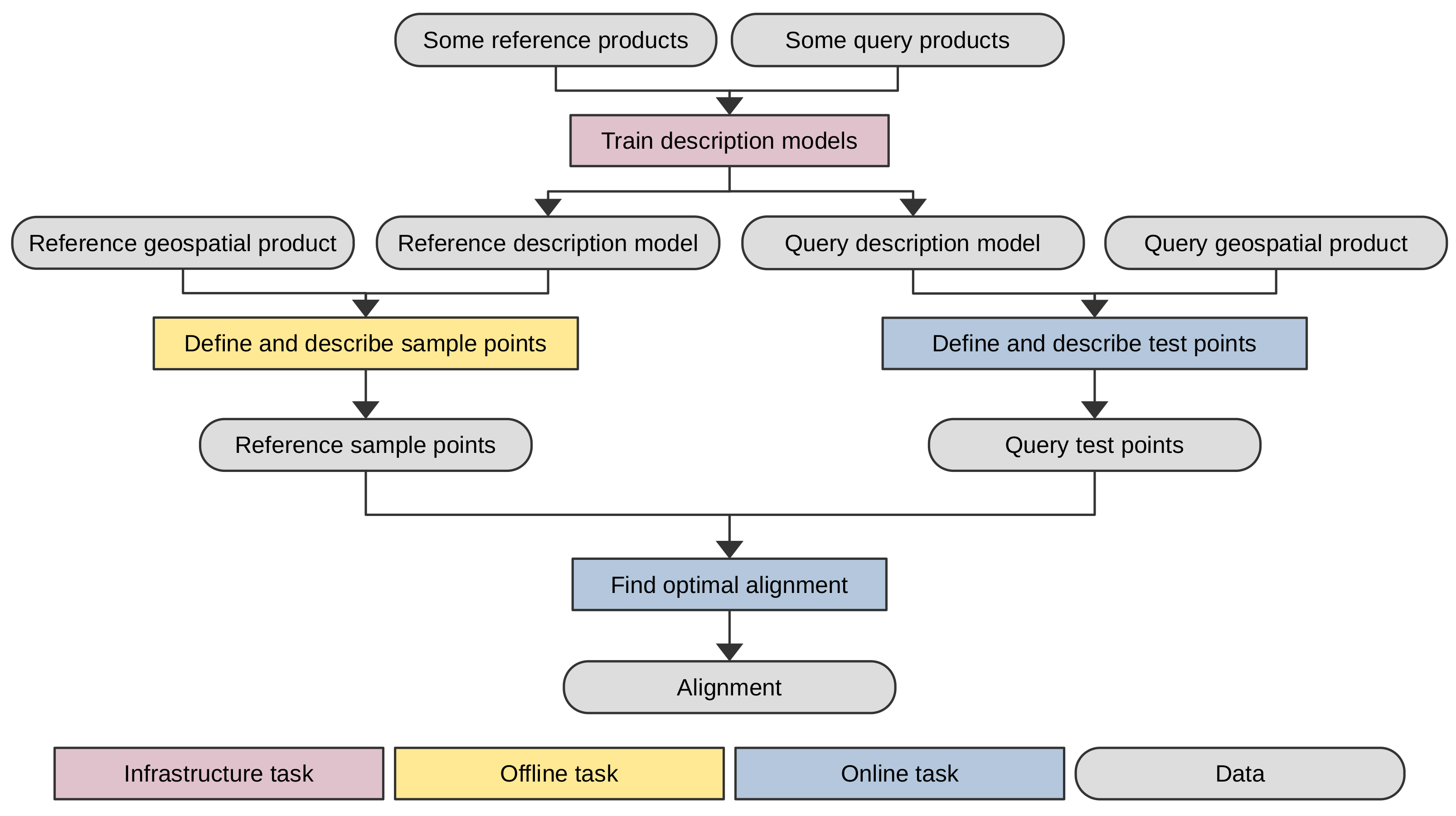
Figure 2 represents the complete fusion process. First (in pink), one trains the description models (i.e., the neural networks) associated with the reference and query modalities. This task requires pairs of colocated geospatial products of the reference and query modalities. Secondly (in yellow), one produces the alignment data. The alignment data are a set of points sampled in the coordinate domain of the reference geographic product and their respective local descriptors. This task can be performed offline and depends on the reference geospatial product and on the reference description model. Thirdly (in blue), given the query remote sensing image and the query description extraction model, one samples points in the coordinate domain of the query remote sensing image, one computes their local descriptors and one finds the minimum of the cost function to infer the mapping between the query and reference coordinate systems.
The online execution time is asymptotically proportional to the reference area and to the query area. The offline execution time is proportional to the reference area. Both the online and the offline phase are fully parallelizable. The online phase exhibits a very simple computational structure.

3. Experiments

3.1. Implementation

We implemented our template matching method as a computer program written in C++ and relying on Torch and OpenCV. Thanks to its object-oriented architecture, our program accommodates all geospatial data modalities generically and can be easily extended to support a new one by defining a patch-rendering process.
The computer with which we developed the method and conducted all the experiments was equipped with an Intel(R) Core(TM) i7-12700 CPU, a GeForce RTX 3080 GPU and 32 Gio of random access memory.

3.2. Data

In this section, we present the data with which we conducted our experiments, and we describe the patch-rendering process of each modality. These data constitute a multimodal stack of five different kinds of geospatial products covering five distinct geographic locations in Germany. These locations have forestial, agrarian, industrial and urban land uses.

3.2.1. Pléiades

Pléiades is a constellation of optical remote sensing satellites. We purchased five true-color ortho-images. Their GSD was 50 cm/pixel.
The patch-rendering process associated with Pléiades images was as follows. First, the image was converted to grayscale. Secondly, the image was warped and resampled into a patch having the requested center, footprint diameter, rotation angle, horizontal and vertical flipping. Thirdly, the patch was normalized to zero mean and unit variance.

3.2.2. Miranda

Miranda is a Ka band SAR imaging RADAR developed by Fraunhofer Institute for High Frequency Physics [31,32,33]. We worked with five images. They were vertically monopolarized. They were acquired with an FMCW waveform, a carrier frequency of 35 GHz and a bandwidth of either 600 MHz or 1000 MHz. They were in ground range geometry and their GSD was 12.5 cm/pixel.
The patch-rendering process associated with Miranda images was as follows. First, the image was warped and resampled into a patch having the requested geometry. Secondly, the patch was converted from intensity to log-intensity. Thirdly, the patch was normalized to zero mean and unit variance.

3.2.3. OpenStreetMap

OpenStreetMap is an open worldwide geographic database together with a rich ecosystem of tools to manipulate its content. We extracted from the OpenStreetMap global archive a few subsets corresponding to our regions of interest in Germany.
The patch-rendering process associated with OpenStreetMap data was as follows. First, a color raster having the requested geometry was rendered using libosmscout, a software library that provides the functionality of drawing OpenStreetMap data. We customized the stylesheet that controlled the drawing appearance and behavior. We notably disabled zoom-conditional drawing, we removed labels and icons, we set all lines to be drawn as solid instead of dashes, and we removed line terminal markers. The rendered patch was finally converted to grayscale and normalized to zero mean and unit variance.

3.2.4. DOP

DOP stands for Digitale OrthoPhotos. It is a collection of airborne optical images covering the entire German territory. As part of the EU open-data directive, the states of Rhineland-Palatinate and North Rhine-Westphalia provide DOP images under an open license. The state of Baden-Wuttemberg currently sells DOP images but plans to provide open access to them by June 2024. The resolutions of the images that we accessed or purchased were 20 cm/pixel and 40 cm/pixel. We produced large rasters whose GSD was 1 m/pixel.
The patch-rendering process associated with the DOP modality was as follows. First, the image was converted to grayscale. Secondly, the image was warped and resampled into a patch having the requested geometry. Thirdly, the patch was normalized to zero mean and unit variance.

3.2.5. KOMPSAT-5

KOMPSAT-5 is a Korean X band SAR imaging earth observation satellite. We purchased two images. Their imaging mode was enhanced standard (ES) stripmap, their processing level was L1D (geocoded with a digital elevation model), and their GSD was 1.1 m. Both their range and azimuth resolution were 2.5 m. One image was vertically polarized while the other was horizontally polarized.
The patch-rendering process associated with the KOMPSAT-5 modality was as follows. First, the image was warped and resampled into a patch having the requested geometry. Secondly, the patch was converted from intensity to log-intensity. Thirdly, the patch was normalized to zero mean and unit variance.

3.3. Protocol

Our experiments consisted in aligning query remote sensing images over reference geospatial products. As query remote sensing images, we used crops extracted from the Pléiades images and from the Miranda images. Their size was 800 m × 800 m (their area was 0.64 km2). These crops were generated using a sliding window with 50% overlap between consecutive windows. As reference geospatial products, we used crops extracted from OpenStreetMap data, from DOP images and from KOMPSAT-5 images. Their size was 15 km × 15 km (their area was 225 km2). The true location of the query crop within the reference crop was random and uniformly distributed (apart from KOMPSAT-5 images because they were not large enough). For one of our five geographic locations, the DOP image was large enough for training description models but not large enough for performing alignment experiments.
For training the description models and for measuring the performance of our algorithm, we manually produced a ground-truth alignment. The produced alignments were either affine transforms or natural neighbor interpolants. It may happen that two superposed geospatial products are locally incoherent. They may have been produced at different times and the content of the scene may have changed in-between. We masked out such areas when training the description models but not when performing the alignments.
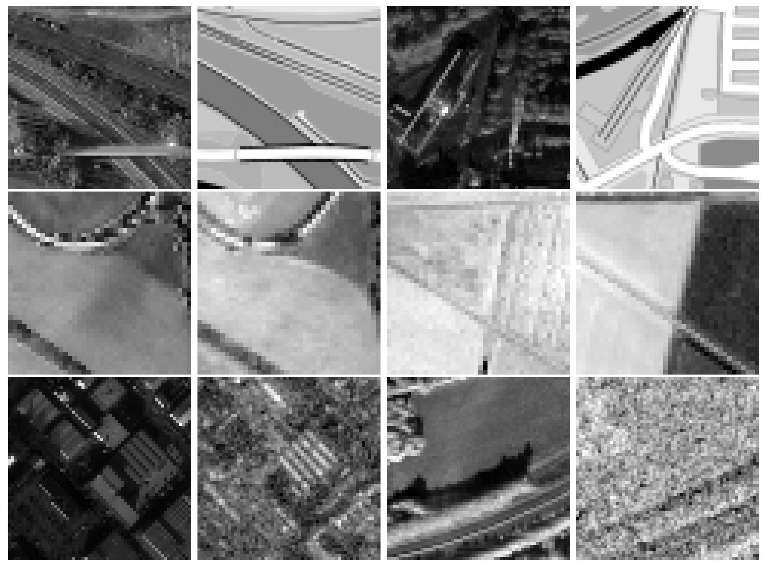
We chose the ground footprint and the raster size of the patches depending on the combination of query and reference modalities. These settings are reported in Table 1. Examples of pairs of raster patches are represented in Figure 3.
We trained a description model for each combination of a query remote sensing image and a reference modality. This amounted to 30 description models. Each description model was tested on its corresponding query remote sensing image and was trained on the other query remote sensing images of the same modality. We could thus perform a cross-validation for each combination of a query modality and a reference modality.
The neural networks were trained using stochastic gradient descent. The learning rate was 10 2 with a decay of 0.95 every four epochs. We considered to hard-mine the negatives j and k but having observed no benefit, we discarded this strategy. The negatives were sampled from the entire dataset. Each batch referenced 128 distinct geographic locations. Given that a geographic location was associated with a positive and a negative patch from the reference and from the query modalities, each batch was accordingly associated with 4 × 128 = 512 descriptors. The number of epochs was 39.

3.4. Results

3.4.1. Local Description Models

The discriminativeness of the trained description models was measured according to the score defined in [34]. It is the probability that two geographically separate descriptors are closer than T in the descriptor space. This threshold was chosen such that the probability of two collocated descriptors being farther apart than T was 5%. These scores are reported in Table 2. The combination of modalities achieving the best scores is Pléiades/DOP. It is the combination whose modality gap is minimal. The combinations of modalities with the worst scores are those involving KOMPSAT-5. The resolution and dynamic range of the KOMPSAT-5 images are significantly worse than those of the other images involved in the experiment.

3.4.2. Alignment

We aligned each crop of a query remote sensing image onto each reference modality. The description model used to align a crop was not trained on the geospatial product to which the crop belonged. We built one piece of alignment data (i.e., one set of reference points and their respective local descriptors) for each combination of a query remote sensing image and a reference modality. Without parallelization, building one piece of alignment data comprising about 8 million points took a few hours. Building the alignment data was fully parallelizable though, so that the execution time could be reduced proportionally to the number of processing units. One piece of alignment data composed of 8 million points took about 4 Gio of storage. Note that each piece of alignment data was shared between several crops and was consequently larger than necessary for a single alignment. Performing an alignment (that is to say, computing the local descriptors from the query and performing the optimization) took between 1.5 and 2 s. The sampling of the cost function was multithreaded. The alignment execution time included the nearest neighbor searches, but these could be precomputed offline.
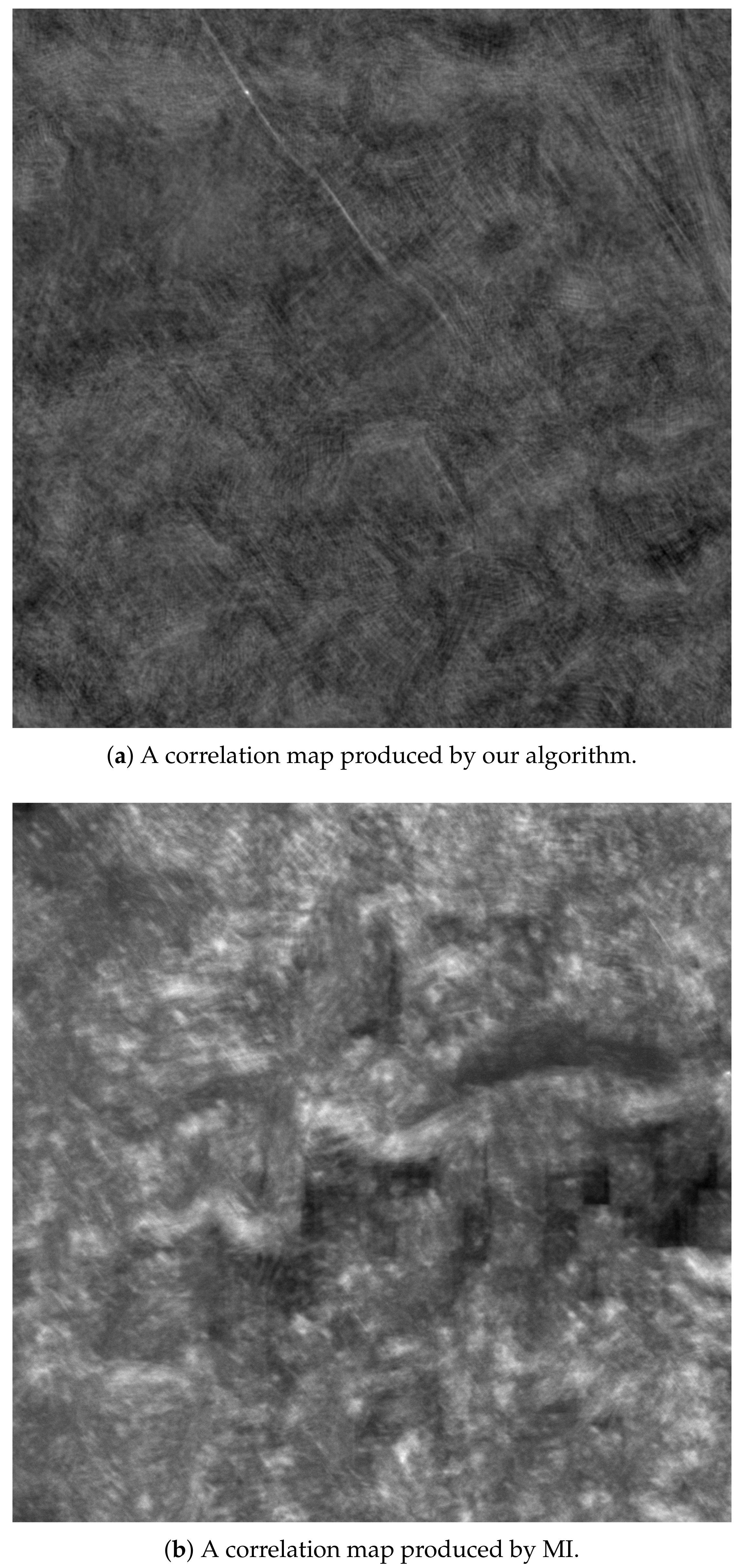
The quality of a superposition produced by our algorithm was measured as follows. For each single alignment experiment, we computed the magnitude of the average offset (i.e., the magnitude of the average difference between the predicted and the ground-truth positions in the coordinate domain of the reference when we took a point uniformly at random in the coordinate domain of the query). In Figure 4, for each combination of data modalities, we report the cumulative distribution of these magnitudes over all the corresponding alignment experiments. These curves indicate the percentage of alignments that achieved a given precision. In Table 3, for each combination of data modalities, we report the number of experiments for which the magnitude of the average offset was lower than 20 m. By convention, we call such alignment experiments successful even though some of them may be imprecise. We also report in Table 3 the success rate for mutual information (MI), normalized cross-correlation (NCC) and channel features of oriented gradient (CFOG). We computed the success rates of these three methods by producing 10 m resolution rasters (for the reference and the query) comparing the pattern with a moving window. Examples of alignments produced by our algorithm are reported in Figure 5. Finally, a correlation map produced using our method and a correlation map produced using MI are reported in Figure 6.
CFOG is a dense descriptor tailored for refining tie points between geospatial products of different modalities [14]. It was introduced and experimentally benchmarked for refining tie points and thus determines a residual deformation field, which is a different use case than ours. Each pixel is associated with one local histogram of gradient orientation. Densely extracting CFOG descriptors involves detecting contours with Sobel filtering (i.e., based on finite differences), building a histogram for each 1 × 1 local neighborhood, depthwise low-pass filtering (to enlarge the local neighborhoods) and pixelwise low-pass filtering (to reduce orientation quantization artefacts). The similarity metric for CFOG is the sum of squared differences, which can be computed quickly by fast convolution using an FFT. Fundamentally, CFOG measures the local similarity of contour orientation. As in the original paper, we used nine orientation bins, a 3 × 3 Sobel kernel, and orientations were modulo 180 degrees.
First, we observed that the traditional methods as well as CFOG failed to obtain satisfying alignment success rates. Mutual information offered much higher success rates than normalized cross-correlation when the reference was OpenStreetMap. For the other references, these two methods offered relatively similar success rates. For the traditional methods, the best scores were achieved on the combination Pléiades-DOP, which had the smallest modality gap. As seen in Figure 6, the correlation map produced by our method is flatter and exhibits a clearer correlation peak than the correlation map produced using MI.
CFOG also failed and proved worse than the traditional methods. We used the same template size and resolution as in [14] but the area of the search window was 315 times larger. Moreover, [14] used many tie points (instead of one), which we could not do because our query remote sensing products were large enough for only one template at that resolution. CFOG relies on Sobel filtering for contour detection, which is sensitive to speckle. However, at the resampled resolution, the speckle of the Miranda images was averaged out and visually imperceptible. Thus, the poor performance of CFOG could not be attributed to the presence of speckle. CFOG relies on contour orientation co-occurrence and not on intensity co-occurrence as MI and NCC. The poor performance of CFOG may be attributed to an unreliability of the multimodal contour detection. A better approach to multimodal alignment based on contours may be to minimize the average distance between the contours. This can be efficiently implemented with chamfer matching [35] or the iterative closest point (ICP) method [36]. However, this approach requires a handcrafted multimodal contour detector, which is not trivial. For instance, the width of the roads in OpenStreetMap is rarely set, so the roads are rendered based on a conventional width and not on a physical width. A metric based on deep learning can handle such discrepancies automatically whereas engineering a handcrafted contour detector that takes it into account would be very difficult.
Our alignment method was able to align geospatial products very robustly despite the size and modality mismatch. The combination of modalities that achieved the best median precision was Pléiades/DOP, which was coherent with the small gap between these two modalities. The worst combination of modalities in terms of the median precision was Miranda/KOMPSAT-5. This may derive from the comparatively poor resolution and dynamic range of our KOMPSAT-5 images. As well, we chose a larger local descriptor footprint for KOMPSAT-5 than for the other modalities, which may have led to less spatially accurate local descriptors. We can order the combinations of modalities as follows in terms of median precision:
  • Pléiades + DOP < Miranda + DOP < Miranda + KOMPSAT-5
  • Pléiades + DOP < Pléiades + KOMPSAT-5 < Miranda + KOMPSAT-5.
Our optical images appeared to be systematically more adequate for alignment than our SAR images. In terms of precision, using OpenStreetMap as a reference was nearly as good as using our optical imagery and was significantly better than using our SAR imagery.
Examining the unsuccessful alignment experiments, we identified the following failure modes: objects unseen at training, temporal inconsistency and poor focusing. A Pléiades crop whose alignment failed contained fields covered by farming tarpaulins unseen at training. A Miranda crop whose alignment failed contained electric lines. They were unseen at training and exhibited some overlap. A Miranda crop whose alignment failed contained hills and was poorly focused.

4. Discussion

4.1. Relation to Image Retrieval

Image retrieval is the task of searching in a database an image that is most similar to a query image. The similarity between a query image and a database image is measured using global image descriptors. Pattern matching can be thought of as image retrieval. In our method, the global descriptor associated with an image is the concatenation of all the local descriptors, and the similarity metric of global descriptors is the squared L2 norm. With traditional NCC and MI methods, the global descriptor associated with an image is the image itself, and the similarity metric of global descriptors is the NCC or the MI. However, with typical image retrieval systems, the global descriptor is obtained by a more complex aggregation of local descriptors, typically via a bag of visual words (BOVW) [37,38] or via a vector of locally aggregated descriptors (VLAD) [39,40].
We are not aware of an image retrieval system that has been experimentally demonstrated to work on such a challenging multimodal dataset as ours. There is little work on multimodal remote sensing image retrieval [41,42], and remote sensing image retrieval systems are generally tested on databases of a few tens of thousands of images. In our method, the distance between two global descriptors is the average point-to-point dissimilarity of the two images, as measured by local descriptors. This property might be lost if the local descriptors were aggregated by a complex process. The matching performance would probably be reduced, and the behavior of the algorithm would be less intuitive. Even if the local descriptors were aggregated by a complex process, we could still not simultaneously improve execution time and memory use, since our local descriptors are shared among global descriptors so that a map of global descriptors and a map of local descriptors would occupy the same volume of memory (provided that the sampling step is the same and that the global and local descriptors have the same dimension). Conversely, our method would perform poorly as an image retrieval method since we generally want image retrieval to be based on content independently of the location of that content within the image. However, a contribution of image retrieval systems to our method could be to use binary code descriptors since they may be more computationally efficient [42].

4.2. Class of Transformations

In our experiments, the retrieved coordinate mapping was a translation. In the context of aerial navigation, the class of transformations between the query and reference geospatial products may be greater than or different from the translations. The translations are sufficient for optical imaging if the altitude and orientation are known, assuming a downward-looking camera. Since our descriptors are covariant with rotation (i.e., the reference and query descriptors still match if their reference and query local raster patches are simultaneously rotated), the class of rigid transforms S E ( 2 ) can be handled straightforwardly by testing different orientations of the map, at the price of an execution time multiplied by the number of orientations considered. Similarly, the descriptors can be made covariant to scale over some range of scales by training the description models over this range of scales. Using the descriptors’ covariance, at the price of an increased execution time and an increased size of the alignment data, we can estimate a plane similitude from S i m ( 2 ) . Finally, although too computationally expensive for real-time use, another way to handle other classes of transformations is to extract new local features from resampled local raster patches. The two approaches can be combined in order to reduce the number of descriptors extractions.

4.3. Real-Time Use

A piece of alignment data cannot be built in real time, at least not with the computational power available on an embedded system or on a desktop computer. However, once the alignment data are built, the alignment can be inferred fast enough for use with the autonomous navigation of an aerial platform such as a missile or a drone.

4.4. Similarity Metric

In this work, the local descriptors were compared with the L 2 norm. The fact that it is unbounded may be detrimental to the alignment success rate. In future works, we shall investigate the use of a bounded local-descriptor similarity metric function such as the composition of the scalar product and the sigmoid or the cosine similarity.

5. Conclusions

We proposed and evaluated a generic system for aligning geospatial products with different modalities. Our system can be extended to new data modalities simply by defining a patch-rendering process. This spares the difficult, time-consuming and unnecessary task of engineering a custom algorithm tailored for a specific modality combination. This system could be applied to the self-localization and autonomous navigation of aerial devices such as missiles and drones.

Author Contributions

Conceptualization, methodology, software, validation, formal analysis, investigation, data curation, writing and editing, V.M.-L.; resources, review, supervision, project administration, funding acquisition, J.-M.L.C. and J.P.-F. All authors have read and agreed to the published version of the manuscript.

Funding

Victor MARTIN-LAC is supported by a CIFRE grant from Agence Nationale de la Recherche Technologique (ANRT).

Data Availability Statement

Restrictions apply to the availability of these data. Pléiades images were purchased through the company SkyWatch. Miranda images were purchased from Fraunhofer Institute For High Frequency Physics (https://www.fhr.fraunhofer.de/, accessed on 20 July 2023). OpenStreetMap data are available under the open database license. Map data are copyrighted by OpenStreetMap contributors and available from https://planet.osm.org/, accessed on 20 July 2023. The DOP images of the states of Rhineland-Palatinate and North Rhine-Westphalia are under a Germany Zero license. The DOP image of the state of Baden-Wuttemberg was purchased from https://www.lgl-bw.de/, accessed on 20 July 2023. KOMPSAT-5 images were purchased and are subject to a license from the Korean Aerospace Institute. They can be purchased from SI Imaging Services (https://www.si-imaging.com/, accessed on 20 July 2023).

Acknowledgments

The authors would like to thank Cécile BAUDRY from Thales Land and Air Systems for her review of this article.

Conflicts of Interest

The authors declare no conflict of interest.

Abbreviations

The following abbreviations are used in this manuscript:
CFOGChannel features of oriented gradient
DOPDigitale OrthoPhotos
DSMACDigital Scene Matching Area Correlator
EUEuropean Union
FFTFast Fourier transform
FMCWFrequency-modulated continuous wave
GSDGround sampling distance
ICPIterative closest point
KOMPSATKOrean MultiPurpose SATellite
MIMutual information
NCCNormalized cross-correlation
RADARRadio detection and ranging
SARSynthetic aperture radar

References

  1. Isola, P.; Zhu, J.Y.; Zhou, T.; Efros, A. Image-to-Image Translation with Conditional Adversarial Networks. In Proceedings of the IEEE Conference on Computer Vision and Pattern Recognition, Honolulu, HI, USA, 21–26 July 2017; pp. 5967–5976. [Google Scholar] [CrossRef]
  2. Rott Shaham, T.; Gharbi, M.; Zhang, R.; Shechtman, E.; Michaeli, T. Spatially-Adaptive Pixelwise Networks for Fast Image Translation. In Proceedings of the Computer Vision and Pattern Recognition (CVPR), Nashville, TN, USA, 20–25 June 2021. [Google Scholar]
  3. Irani, G.; Christ, H. Image Processing for Tomahawk Scene Matching. Johns Hopkins APL Tech. Dig. 1994, 15, 250–264. [Google Scholar]
  4. Costea, D.; Leordeanu, M. Aerial image geolocalization from recognition and matching of roads and intersections. arXiv 2016, arXiv:1605.08323. [Google Scholar]
  5. Kovesi, P. Image Features From Phase Congruency. Videre J. Comput. Vis. Res. 1995, 1, 31. [Google Scholar]
  6. Yu, G.; Zhao, S. A New Feature Descriptor for Multimodal Image Registration Using Phase Congruency. Sensors 2020, 20, 5105. [Google Scholar] [CrossRef] [PubMed]
  7. Ye, Y.; Shan, J.; Bruzzone, L.; Shen, L. Robust Registration of Multimodal Remote Sensing Images Based on Structural Similarity. IEEE Trans. Geosci. Remote Sens. 2017, 55, 2941–2958. [Google Scholar] [CrossRef]
  8. Xiang, Y.; Tao, R.; Wang, F.; You, H.; Han, B. Automatic Registration of Optical and SAR Images Via Improved Phase Congruency Model. IEEE J. Sel. Top. Appl. Earth Obs. Remote Sens. 2020, 13, 5847–5861. [Google Scholar] [CrossRef]
  9. Xiang, Y.; Wang, F.; Wan, L.; You, H. SAR-PC: Edge Detection in SAR Images via an Advanced Phase Congruency Model. Remote Sens. 2017, 9, 209. [Google Scholar] [CrossRef]
  10. Wang, L.; Sun, M.; Liu, J.; Cao, L.; Ma, G. A Robust Algorithm Based on Phase Congruency for Optical and SAR Image Registration in Suburban Areas. Remote Sens. 2020, 12, 3339. [Google Scholar] [CrossRef]
  11. Ragb, H.K.; Asari, V.K. Histogram of oriented phase (HOP): A new descriptor based on phase congruency. In Mobile Multimedia/Image Processing, Security, and Applications 2016; SPIE: Bellingham, WA, USA, 2016; Volume 9869, pp. 192–201. [Google Scholar] [CrossRef]
  12. Dellinger, F.; Delon, J.; Gousseau, Y.; Michel, J.; Tupin, F. SAR-SIFT: A SIFT-Like Algorithm for SAR Images. IEEE Trans. Geosci. Remote Sens. 2015, 53, 453–466. [Google Scholar] [CrossRef]
  13. Lowe, D.G. Distinctive Image Features from Scale-Invariant Keypoints. Int. J. Comput. Vis. 2004, 60, 91–110. [Google Scholar] [CrossRef]
  14. Ye, Y.; Bruzzone, L.; Shan, J.; Bovolo, F.; Zhu, Q. Fast and Robust Matching for Multimodal Remote Sensing Image Registration. IEEE Trans. Geosci. Remote Sens. 2019, 57, 9059–9070. [Google Scholar] [CrossRef]
  15. Xiong, X.; Xu, Q.; Jin, G.; Zhang, H.; Gao, X. Rank-Based Local Self-Similarity Descriptor for Optical-to-SAR Image Matching. IEEE Geosci. Remote Sens. Lett. 2020, 17, 1742–1746. [Google Scholar] [CrossRef]
  16. Shechtman, E.; Irani, M. Matching Local Self-Similarities across Images and Videos. In Proceedings of the 2007 IEEE Conference on Computer Vision and Pattern Recognition, Minneapolis, MN, USA, 18–23 June 2007; pp. 1–8. [Google Scholar] [CrossRef]
  17. Hoffer, E.; Ailon, N. Deep metric learning using Triplet network. arXiv 2018, arXiv:1412.6622. [Google Scholar]
  18. Simo-Serra, E.; Trulls, E.; Ferraz, L.; Kokkinos, I.; Fua, P.; Moreno-Noguer, F. Discriminative Learning of Deep Convolutional Feature Point Descriptors. In Proceedings of the 2015 IEEE International Conference on Computer Vision (ICCV), Washington, DC, USA, 7–13 December 2015; IEEE: Santiago, Chile, 2015; pp. 118–126. [Google Scholar] [CrossRef]
  19. Mishchuk, A.; Mishkin, D.; Radenovic, F.; Matas, J. Working hard to know your neighbor’s margins: Local descriptor learning loss. In Proceedings of the Advances in Neural Information Processing Systems; Curran Associates, Inc.: Red Hook, NY, USA, 2017; Volume 30. [Google Scholar]
  20. Zagoruyko, S.; Komodakis, N. Learning to Compare Image Patches via Convolutional Neural Networks. arXiv 2015, arXiv:1504.03641. [Google Scholar]
  21. Han, X.; Leung, T.; Jia, Y.; Sukthankar, R.; Berg, A.C. MatchNet: Unifying feature and metric learning for patch-based matching. In Proceedings of the 2015 IEEE Conference on Computer Vision and Pattern Recognition (CVPR), Boston, MA, USA, 7–12 June 2015; IEEE: Boston, MA, USA, 2015; pp. 3279–3286. [Google Scholar] [CrossRef]
  22. Tian, Y.; Fan, B.; Wu, F. L2-Net: Deep Learning of Discriminative Patch Descriptor in Euclidean Space. In Proceedings of the 2017 IEEE Conference on Computer Vision and Pattern Recognition (CVPR), Honolulu, HI, USA, 21–26 July 2017; pp. 6128–6136. [Google Scholar] [CrossRef]
  23. Balntas, V.; Johns, E.; Tang, L.; Mikolajczyk, K. PN-Net: Conjoined Triple Deep Network for Learning Local Image Descriptors. arXiv 2016, arXiv:1601.05030. [Google Scholar]
  24. Hughes, L.H.; Schmitt, M.; Mou, L.; Wang, Y.; Zhu, X.X. Identifying Corresponding Patches in SAR and Optical Images With a Pseudo-Siamese CNN. IEEE Geosci. Remote Sens. Lett. 2018, 15, 784–788. [Google Scholar] [CrossRef]
  25. Hughes, L.; Schmitt, M.; Zhu, X. Mining Hard Negative Samples for SAR-Optical Image Matching Using Generative Adversarial Networks. Remote Sens. 2018, 10, 1552. [Google Scholar] [CrossRef]
  26. Hughes, L.H.; Merkle, N.; Bürgmann, T.; Auer, S.; Schmitt, M. Deep Learning for SAR-Optical Image Matching. In Proceedings of the IGARSS 2019—2019 IEEE International Geoscience and Remote Sensing Symposium, Yokohama, Japan, 28 July–2 August 2019; pp. 4877–4880. [Google Scholar] [CrossRef]
  27. Hughes, L.H.; Marcos, D.; Lobry, S.; Tuia, D.; Schmitt, M. A deep learning framework for matching of SAR and optical imagery. ISPRS J. Photogramm. Remote Sens. 2020, 169, 166–179. [Google Scholar] [CrossRef]
  28. Liao, Y.; Di, Y.; Zhou, H.; Li, A.; Liu, J.; Lu, M.; Duan, Q. Feature Matching and Position Matching Between Optical and SAR With Local Deep Feature Descriptor. IEEE J. Sel. Top. Appl. Earth Obs. Remote Sens. 2022, 15, 448–462. [Google Scholar] [CrossRef]
  29. Bürgmann, T.; Koppe, W.; Schmitt, M. Matching of TerraSAR-X derived ground control points to optical image patches using deep learning | Elsevier Enhanced Reader. ISPRS J. Photogramm. Remote Sens. 2019, 158, 241–248. [Google Scholar] [CrossRef]
  30. Zhang, M.; Li, W.; Tao, R.; Wang, S. Transfer Learning for Optical and SAR Data Correspondence Identification with Limited Training Labels. IEEE J. Sel. Top. Appl. Earth Obs. Remote Sens. 2021, 14, 1545–1557. [Google Scholar] [CrossRef]
  31. Frioud, M.; Wahlen, A.; Wellig, P.; Meier, E. Processing of MIRANDA35 FMCW-SAR Data using a Time-Domain Algorithm. In Proceedings of the EUSAR 2014, 10th European Conference on Synthetic Aperture Radar, Berlin, Germany, 2–6 June 2014; pp. 1–4. [Google Scholar]
  32. Stanko, S.; Johannes, W.; Sommer, R.; Wahlen, A.; Wilcke, J.; Essen, H.; Tessmann, A.; Kallfass, I. SAR with MIRANDA—Millimeterwave radar using analog and new digital approach. In Proceedings of the 2011 8th European Radar Conference, Manchester, UK, 12–14 October 2011; pp. 214–217. [Google Scholar]
  33. Henke, D.; Frioud, M.; Fagir, J.; Guillaume, S.; Meindl, M.; Geiger, A.; Sieger, S.; Janssen, D.; Klöppel, F.; Caris, M.; et al. Miranda35 Experiments in Preparation for Small Uav-Based Sar. In Proceedings of the IGARSS 2019—2019 IEEE International Geoscience and Remote Sensing Symposium, Yokohama, Japan, 28 July–2 August 2019; pp. 8542–8545. [Google Scholar] [CrossRef]
  34. Mikolajczyk, K.; Schmid, C. A Performance Evaluation of Local Descriptors. IEEE Trans. Pattern Anal. Mach. Intell. 2005, 27, 16. [Google Scholar] [CrossRef] [PubMed]
  35. Sjanic, Z.; Gustafsson, F. Navigation and SAR focusing with map aiding. IEEE Trans. Aerosp. Electron. Syst. 2015, 51, 1652–1663. [Google Scholar] [CrossRef]
  36. Markiewicz, J.; Abratkiewicz, K.; Gromek, A.; Ostrowski, W.; Samczyński, P.; Gromek, D. Geometrical Matching of SAR and Optical Images Utilizing ASIFT Features for SAR-based Navigation Aided Systems. Sensors 2019, 19, 5500. [Google Scholar] [CrossRef] [PubMed]
  37. Sivic, Z. Video Google: A text retrieval approach to object matching in videos. In Proceedings of the Ninth IEEE International Conference on Computer Vision, Sardinia, Italy, 13–16 October 2003; Volume 2, pp. 1470–1477. [Google Scholar] [CrossRef]
  38. Yang, Y.; Newsam, S. Geographic Image Retrieval Using Local Invariant Features. IEEE Trans. Geosci. Remote Sens. 2013, 51, 818–832. [Google Scholar] [CrossRef]
  39. Jégou, H.; Douze, M.; Schmid, C.; Pérez, P. Aggregating local descriptors into a compact image representation. In Proceedings of the 2010 IEEE Computer Society Conference on Computer Vision and Pattern Recognition, San Francisco, CA, USA, 13–18 June 2010; pp. 3304–3311. [Google Scholar] [CrossRef]
  40. Imbriaco, R.; Sebastian, C.; Bondarev, E.; de With, P.H.N. Aggregated Deep Local Features for Remote Sensing Image Retrieval. Remote Sens. 2019, 11, 493. [Google Scholar] [CrossRef]
  41. Zhou, W.; Guan, H.; Li, Z.; Shao, Z.; Delavar, M.R. Remote Sensing Image Retrieval in the Past Decade: Achievements, Challenges, and Future Directions. IEEE J. Sel. Top. Appl. Earth Obs. Remote Sens. 2023, 16, 1447–1473. [Google Scholar] [CrossRef]
  42. Xiong, W.; Xiong, Z.; Zhang, Y.; Cui, Y.; Gu, X. A Deep Cross-Modality Hashing Network for SAR and Optical Remote Sensing Images Retrieval. IEEE J. Sel. Top. Appl. Earth Obs. Remote Sens. 2020, 13, 5284–5296. [Google Scholar] [CrossRef]
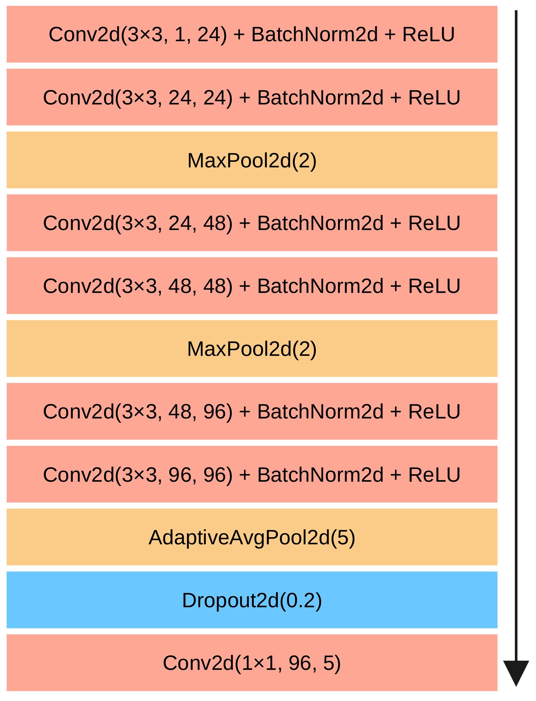
Figure 1. Neural network architecture.
Remotesensing 15 04510 g001
Figure 2. Fusion process.
Remotesensing 15 04510 g002
Figure 3. Examples of pairs of raster patches. From left to right and from top to bottom: Pleiades/OpenStreetMap, Miranda/OpenStreetMap, Pleiades/DOP, Miranda/DOP, Pleiades/KOMPSAT-5 and Miranda/KOMPSAT-5.
Remotesensing 15 04510 g003
Figure 4. Alignment precision.
Remotesensing 15 04510 g004
Figure 5. Examples of alignments. The rectangle represents the footprint of the reference geospatial product over which to align the query. Examples I and II are Pléiades/OpenStreetMap. Example III is Miranda/KOMPSAT-5.
Remotesensing 15 04510 g005
Figure 6. A correlation map produced using our method and a correlation map produced using MI. The modality combination is Pléiades/DOP. The geographic location is the same and its area is (15 km)2. White means higher correlation. Black means lower correlation. The correlation scores were affinely transformed to the range [0, 1]. Note the clean dot on the first correlation map and the more chaotic nature of the second correlation map.
Remotesensing 15 04510 g006
Table 1. Patch footprint diameter and patch size for each combination of query and reference modalities.
Query ModalityReference ModalityPatch FootprintPatch Size
PléiadesOpenStreetMap(150 m)2(60 px)2
PléiadesDOP(150 m)2(40 px)2
PléiadesKOMPSAT-5(200 m)2(60 px)2
MirandaOpenStreetMap(150 m)2(60 px)2
MirandaDOP(150 m)2(40 px)2
MirandaKOMPSAT-5(200 m)2(60 px)2
Table 2. False positive rate for a false negative rate of 5%.
Query ImageFalse Positive Rate
(OpenStreetMap)
False Positive Rate
(DOP)
False Positive Rate
(KOMPSAT-5)
Miranda A0.150.250.35
Miranda B0.030.010.04
Miranda C0.280.230.31
Miranda D0.330.110.20
Miranda E0.280.290.47
Miranda (mean)0.220.180.27
Pléiades A0.110.220.33
Pléiades B0.270.290.24
Pléiades C0.190.080.22
Pléiades D0.130.020.25
Pléiades E0.080.070.22
Pléiades (mean)0.160.140.25
Table 3. Alignment success rate.
Query ModalityReference ModalityNumber of ExperimentsSuccess Rate (Our Method)Success Rate (MI)Success Rate (NCC)Success Rate (CFOG)
PléiadesOpenStreetMap74100%33.0%1.1%0.0%
PléiadesDOP74100%63.5%45.9%16.2%
PléiadesKOMPSAT59494%3.2%1.1%0.0%
MirandaOpenStreetMap4698%11.1%1.9%0.0%
MirandaDOP45100%4.4%6.7%0.0%
MirandaKOMPSAT54878%14.6%14.6%8.3%
Disclaimer/Publisher’s Note: The statements, opinions and data contained in all publications are solely those of the individual author(s) and contributor(s) and not of MDPI and/or the editor(s). MDPI and/or the editor(s) disclaim responsibility for any injury to people or property resulting from any ideas, methods, instructions or products referred to in the content.