Research on the Response Characteristics and Identification of Infrasound Signals in the Jialongcuo Ice Avalanche, Tibet

Abstract

Due to the inability of remote sensing satellites to monitor avalanches in real time, this study focuses on the glaciers in the rear edge of Jialongcuo, Tibet, and uses infrasound sensors to conduct real-time monitoring of ice avalanches. The following conclusions are drawn: (1) In terms of waveform, compared to background noise, ice avalanche events have a slight left deviation and a slightly steep shape; compared to wind, rain, and floods events, ice avalanche events have less obvious kurtosis and skewness. (2) In terms of frequency distribution, the infrasound frequency generated by ice avalanche events is mainly distributed in the range of 1.5 Hz to 9.5 Hz; compared to other events, ice avalanche events differ some in frequency characteristics. (3) The model based on information entropy and marginal spectral frequency distribution characteristics of infrasound have higher accuracy in signal classification and recognition, as they can better represent the differences between infrasound signals of different events than other features. (4) Compared with the K-nearest neighbor algorithm and classification tree algorithm, the support vector machine and BP (Back Propagation) neural network algorithm are more suitable for identifying infrasound signals in the Jialongcuo ice avalanche. The research results can provide theoretical support for the application of infrasound-based ice avalanche monitoring technology.

1. Introduction

Glaciers are widely distributed in the Qinghai–Tibet Plateau, which is rich in fresh water resources, which can meet the survival needs of about 1/3 of people all over the world, so it is also known as the “Asian Water Tower”. The Qinghai–Tibet Plateau serves as a regulator of climate change in the Northern Hemisphere. It provides important ecosystem services for the Asian region. Affected by global warming, glaciers in the Qinghai–Tibet Plateau are melting and retreating. At the same time, the influence of topography, earthquakes, precipitation, and other internal and external forces further increases the probability of ice avalanche disasters [1,2,3]. An ice avalanche is an instant collapse of the ice body in front of a glacier under the action of gravity, which often occurs at the end of the glacier, and sometimes in the middle and upper part of the glacier associated with ice falls [4]. Ice avalanches easily lead to a series of glacier disasters, such as ice lake collapse, debris flow, and plateau landslides [2,3,5,6], which not only affect the ecological environment of the plateau, but also seriously threaten the life and property safety of the people in the plateau and reduce the service function of the ecosystem.

Records of ice avalanches originated in 1767 from Saussure, a Swiss geologist, meteorologist, and mountaineer, who first recorded in detail the movement and ice avalanche phenomena of Alpine glaciers during mountaineering [7]. D.R. Crandell divided ice avalanches into four types in 1968, and ice avalanches belong to one of them [2]. In the same year, Pinchak [8] made a preliminary study on the ice avalanche probability of Vaughan Lewis Glacier. Hans [9] classified ice avalanches in terms of volume and distance of movement. Margreth et al. [10] conducted an ice avalanche hazard assessment based on the Gutzgletscher ice avalanche northwest of Wetterhorn above Greendewa (Bern Alps, Switzerland) in September 1996 and January 1997, and analyzed the formation mechanism and research difficulties of the ice avalanche. It is considered that the ice avalanche is the process of the ice body breaking from the glacier and then falling to the slope and forming small pieces of ice under the action of gravity. With the in-depth understanding of the ice avalanche, researchers began to study and monitor the activity of the ice avalanche. Salzmann et al. [11] developed a method to detect potentially hazardous areas based on statistical parameters, geographic information system (GIS) modeling technology, and remote sensing technology. Vilajosana et al. [12] use seismographs to observe and estimate the energy transferred to the ground by ice avalanches, which is used to verify the model and evaluate the size and classification of ice avalanches. Herwijnen et al. [13] use seismic sensors combined with automatic cameras to monitor ice avalanches to predict ice avalanche activity. Murayama et al. [14] monitored ice shocks through an infrasound array deployed in the bay of eastern Antarctica and found that ice shocks produce special infrasound signals, and ice avalanches are one of the causes of ice shocks and special infrasound. Asming et al. [15] also carried out infrasound monitoring of glaciers in the Arctic and Svalbard, which once again proved that infrasound can be used to monitor glacier damage. Mayer et al. [16] also monitor ice avalanche activity through different infrasound detection systems installed in the Swiss Alps. Herwijnen et al. [13] monitored ice avalanches by infrasound array and evaluated the avalanche activity near the avalanche area by machine learning. Graveline et al. [17] indicated that there may be interaction between ice avalanches and snowslides. Compared with the research on ice avalanche disasters worldwide, there are fewer studies on individual ice avalanche disasters in China, and more on secondary disasters, such as glacial lake collapse and glacier debris flow caused by ice avalanches. Scholars [18,19,20,21] analyzed a large number of ice lake collapse events in Tibet, which proved that ice avalanches were one of the main factors leading to ice lake collapse.

At present, research methods for ice avalanche disasters mainly include site investigation, remote sensing, seismograph, and numerical simulation [12,13]. As ice avalanche disasters often occur in remote mountainous areas with rugged terrain, site investigation is very difficult and dangerous, so the actual data collected are very limited. The development of remote sensing technology has promoted the research on ice avalanche disasters. Remote sensing images can monitor glaciers in all directions, but remote sensing technology relies on the temporal and spatial resolution of satellites and cannot monitor glaciers in real time. Seismographs are mainly used to record the frequency of avalanche events currently, but do not record the whole dynamic process of avalanches. Numerical simulation can simulate the main factors influencing the avalanche, but it is still difficult to simulate the mechanism of an avalanche. In view of this situation, taking the trailing edge glacier of Jialongcuo in Tibet as the research object, infrasound with the characteristics of low frequency, low attenuation, and long propagation distance [22,23,24,25] is used to monitor ice avalanches in this work. On this basis, combined with other monitoring data, features of avalanche infrasound signals were extracted, and avalanche infrasound signals were sorted out from signals of other events to provide technical support for follow-up monitoring and early warning of secondary disasters (ice lake collapse and glacier debris flow, etc.). The infrasound monitoring of ice avalanches can make up for the deficiency of remote sensing technology and realize real-time monitoring of ice avalanche disasters.

2. Methods

2.1. Study Area

2.1.1. Geographical Location

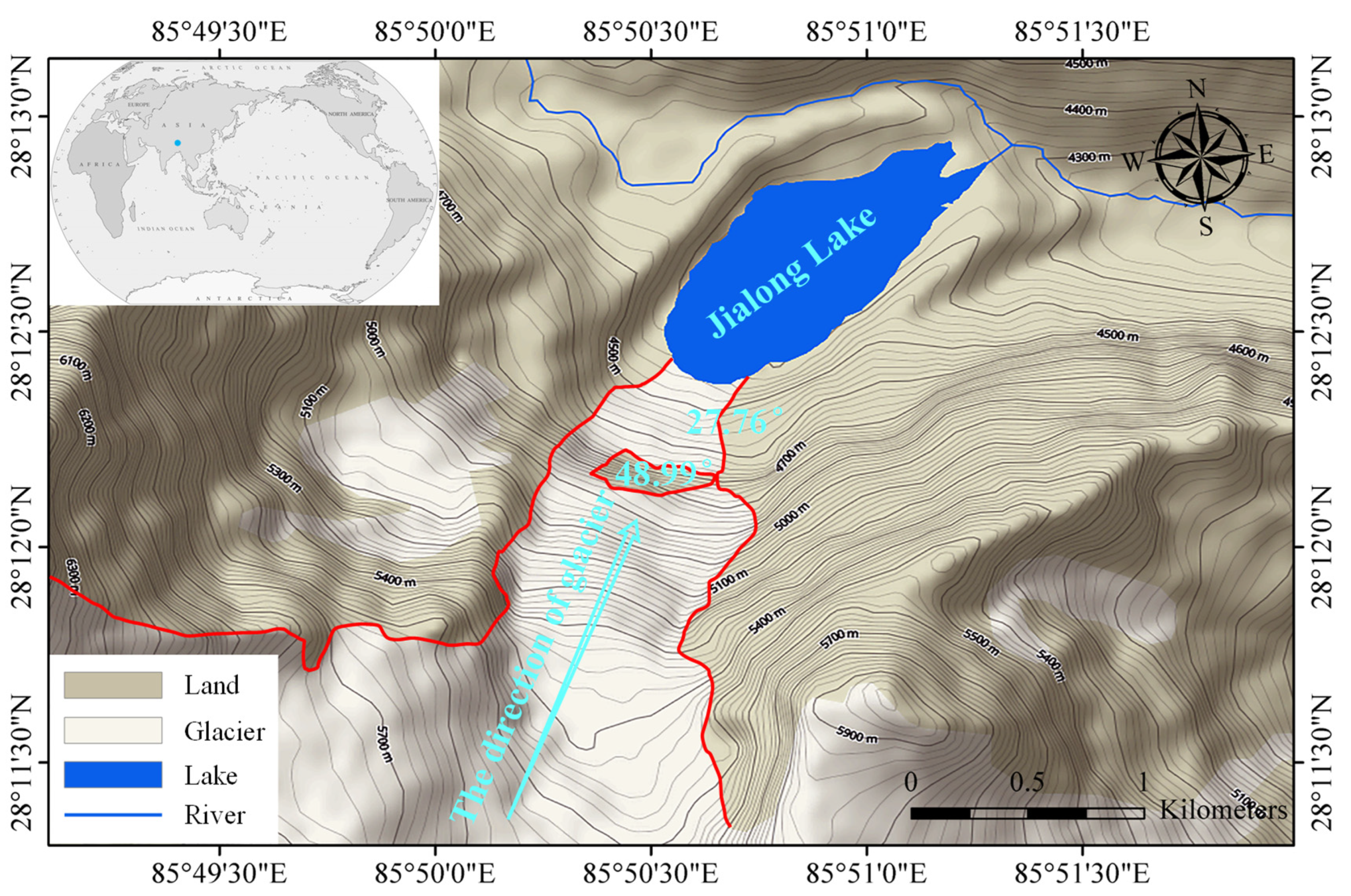
The Jialong Cuo trailing margin glacier belongs to the middle part of the Himalayas, and its watershed code is 50191B. According to the second round of glacier statistics, this glacier is about 4.52 square kilometers in area and about 0.30 cubic kilometers in volume (based on the average estimated volume of the two rounds). The glacier has a maximum elevation of 6660.7 m, a minimum elevation of 4384.2 m, and an average elevation of 5593.6 m, an average slope direction of 56.0 degrees, and an average slope of 27.6 degrees (the above data are from the second catalogue of glaciers in Tibet), as shown in Figure 1.

According to the classification of Chinese glaciers by Chinese glaciologist and academician Shi Yafeng, the upper glacier of Jialongcuo belongs to continental glacier or cold glacier. With a low temperature, dry climate, less precipitation, and weaker water vapor cycle than that on the southern slope of the Himalayas, it has slow movement and weak activity.

2.1.2. Climate

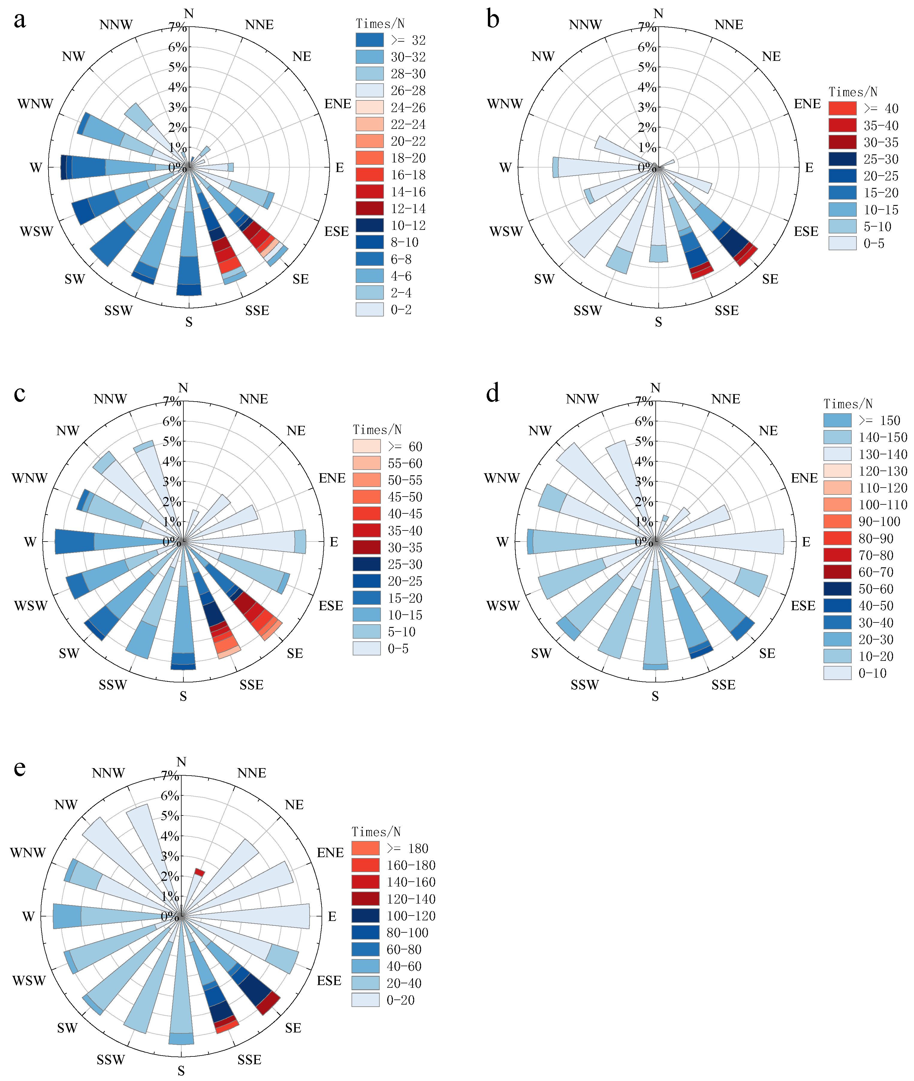
A set of weather stations has been set up in the study area, and meteorological data from 5 November 2020 to 19 January 2022 have been collected. Temperature, air humidity, and wind direction data were processed and analyzed in this work, as shown in Figure 2.

The monitoring results show that the annual temperature in the study area is less than 15 degrees Celsius, and the temperature varies widely from day to night. And, the daily temperature reaches the highest between 12:00 and 14:00. Opposite to air temperature, the relative humidity of the air falls with the rise of temperature, as the water in the air decreases due to evaporation, while sporadic light rain in the evening and night make the moisture content in the air increase.

It can be seen from Figure 3 that southeasterly winds prevail in the study area, which is closely related to the geographical location of the monitoring point. Except for a channel in the southeast, the monitoring point is surrounded by high mountains in the other directions, and thus has weak air circulation overall. Affected by the Indian Ocean monsoon in summer, a small amount of warm and wet air rises along the Zhangmu channel to the southeast of the monitoring point, so it mainly has southeasterly winds in the summer.

2.1.3. Earthquake

According to the statistics of the earthquakes that have occurred in the range of 200 km around the monitoring site since 2021, as shown in

Table 1. Statistics on earthquakes from January 2021 to February 2022.

Seismogenic Time	Earthquake Magnitude/M	Latitude/°	Longitude/°	Focal Depth/km	Reference Position
15 December 2021 04:07:12	3.5	28.59	87.41	10	Dingri County, Rikaze City, Tibet
8 December 2021 12:23:19	3.2	28.77	87.35	10	Dingri County, Rikaze City, Tibet
5 November 2021 09:48:30	4.2	28.73	87.44	10	Dingri County, Rikaze City, Tibet
18 October 2021 18:32:16	3.8	28.54	87.41	10	Dingri County, Rikaze City, Tibet
15 October 2021 18:35:39	3.0	28.64	87.43	10	Dingri County, Rikaze City, Tibet
21 June 2021 18:06:50	3.0	29.3	87.36	10	Angren County, Rikaze City, Tibet
20 June 2021 04:01:39	3.8	29.58	84.3	10	Zhongba County, Rikaze City, Tibet
26 May 2021 04:46:08	4.2	28.99	86.47	10	Nielamu County, Rikaze City, Tibet
16 March 2021 21:16:08	3.4	30.11	86.44	10	Angren County, Rikaze City, Tibet
28 February 2021 04:03:43	3.1	29.07	86.75	10	Dingri County, Rikaze City, Tibet
20 February 2021 02:44:03	3.2	28.79	87.47	17	Dingri County, Rikaze City, Tibet
9 February 2021 09:50:11	3.3	28.01	87.9	10	Dingjie County, Rikaze City, Tibet
4 February 2021 13:06:23	4.3	28.64	87.52	28	Dingri County, Rikaze City, Tibet
2 February 2021 10:31:15	4.7	28.55	87.5	10	Dingri County, Rikaze City, Tibet

, there are 0 earthquakes with magnitude ≥ 5.0 M, 4 earthquakes with magnitude ≥ 4.0 M, and 10 earthquakes with magnitude < 4.0 M in the whole year. On 21 August 2023, at 16:51:59, the epicenter center closest to the monitoring point (Nie Lamu County earthquake with magnitude 4.2) was approximately 118 km away. Therefore, the earthquake may have some impact on potentially unstable glaciers.

2.1.4. Topographic Factor

As shown in Figure 1, the part circled by the red line in the picture is the monitored glacier, which moves toward the glacial lake. The ice tongue of the glacier is about 4880 m in elevation, about 430 m vertically to the ice lake surface, and about 230 m vertically to the position of the steps (surrounded by orange thin strips in the picture). The corresponding angle of the ice tongue at the steps is about 48.99°, exceeding the limit slope of a cold glacier (45°). The steps are 200 m vertically from the lake surface, and the slope of the ice tongue in this section is about 27.76°. The slope of the ice tongue is steep on the whole, which is not conducive to the stability of the glacier.

2.1.5. Disaster Form

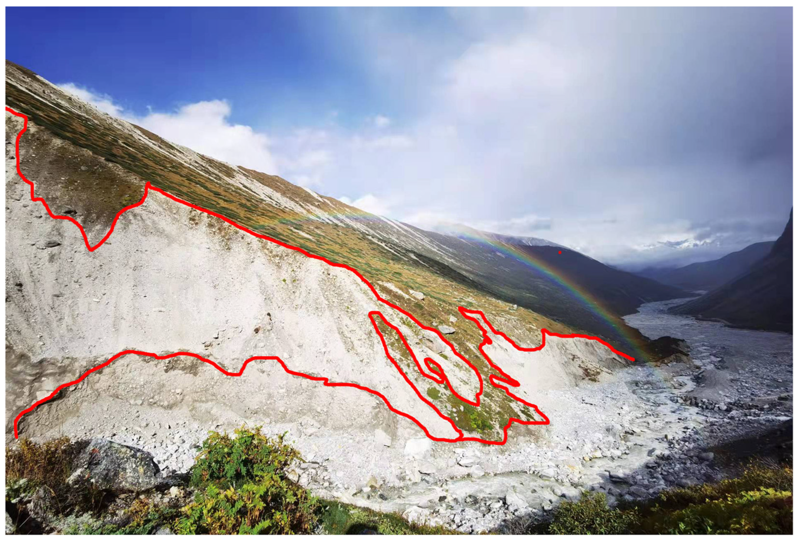
Due to the steep slope at the first step of the glacier, if large amounts of ice fall, they will directly gush into the ice lake and cause surges, which may cause the spillway to burst. The spillway has a height difference of about 40 m with the river and is nearly perpendicular to the other side of the river bank. When a surge instantly rushes into the river and hits the slope of the opposite bank, this part of the bank with loose soil may experience landslides or collapses (Figure 4), causing slope instability and providing large amounts of material sources for debris flow. That is to say, the form of the disaster chain is ice avalanche–ice lake collapse–debris flow. The debris flow formed by the collapse of the ice lake is sudden, which is often accompanied by erosion on both sides of the channel, resulting in the collapse of soil on both sides of the channel, the destruction of vegetation, and the flooding of pastures in areas with flat terrain, causing damage to the ecological environment and posing a threat to the lives and property of local residents. According to the literature records, in May and June 2002, there were two ice avalanches into the Jialongcuo lake, which led to collapses of the ice lake and debris flow disasters.

2.2. Data Collection

2.2.1. Overview of Equipment Layout

The monitoring equipment is installed in Jialong Cuo, Nyalamu County, Rikaze City, Tibet Autonomous region, at the latitude 28°12′24.55″–28°12′54.13″N, longitude 85°51′00.63″–85°51′11.48″E, and about 4376 m above sea level.

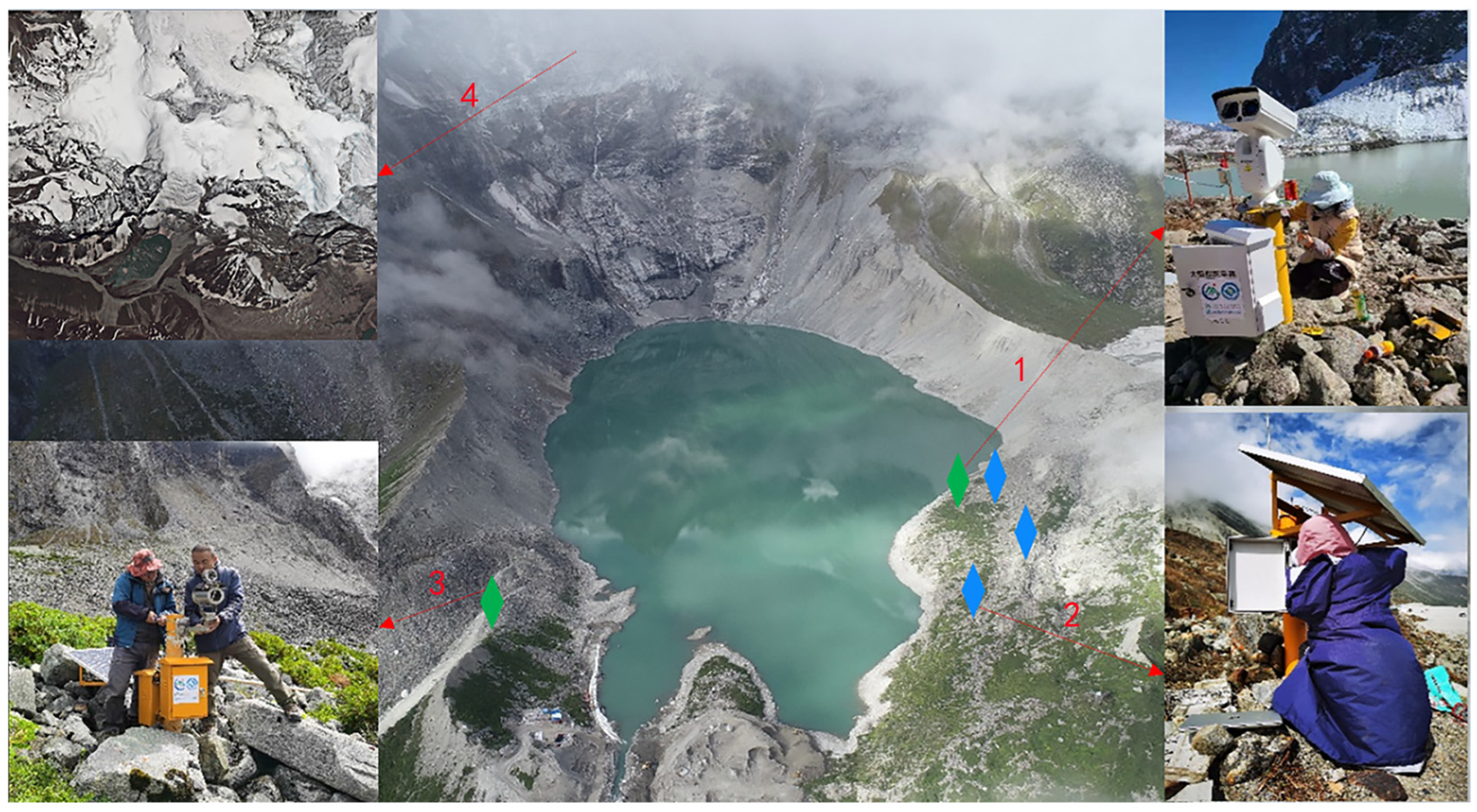
As shown in Figure 5, the blue marks are the positions of infrasound monitoring equipment (corresponding to 2 in the figure). Three sets of infrasound monitoring equipment are installed to form an infrasound array, and the sensors are all facing the glacier (corresponding to 4 in the figure) in the rear edge of Jialongcuo. The infrasound array can effectively reduce the interference of background noise and improve the signal-to-noise ratio of the signals. The green marks are the position where the cameras are; the camera on the right side of the lake (corresponding to 1 in the figure) is used to cooperate with infrasound monitoring equipment to monitor the glacier dynamics, and the camera on the left side of the lake (corresponding to 3 in the figure) is used to monitor whether there are surges and bursts at the overflow mouth of the ice lake.

2.2.2. Infrasound Signal Acquisition

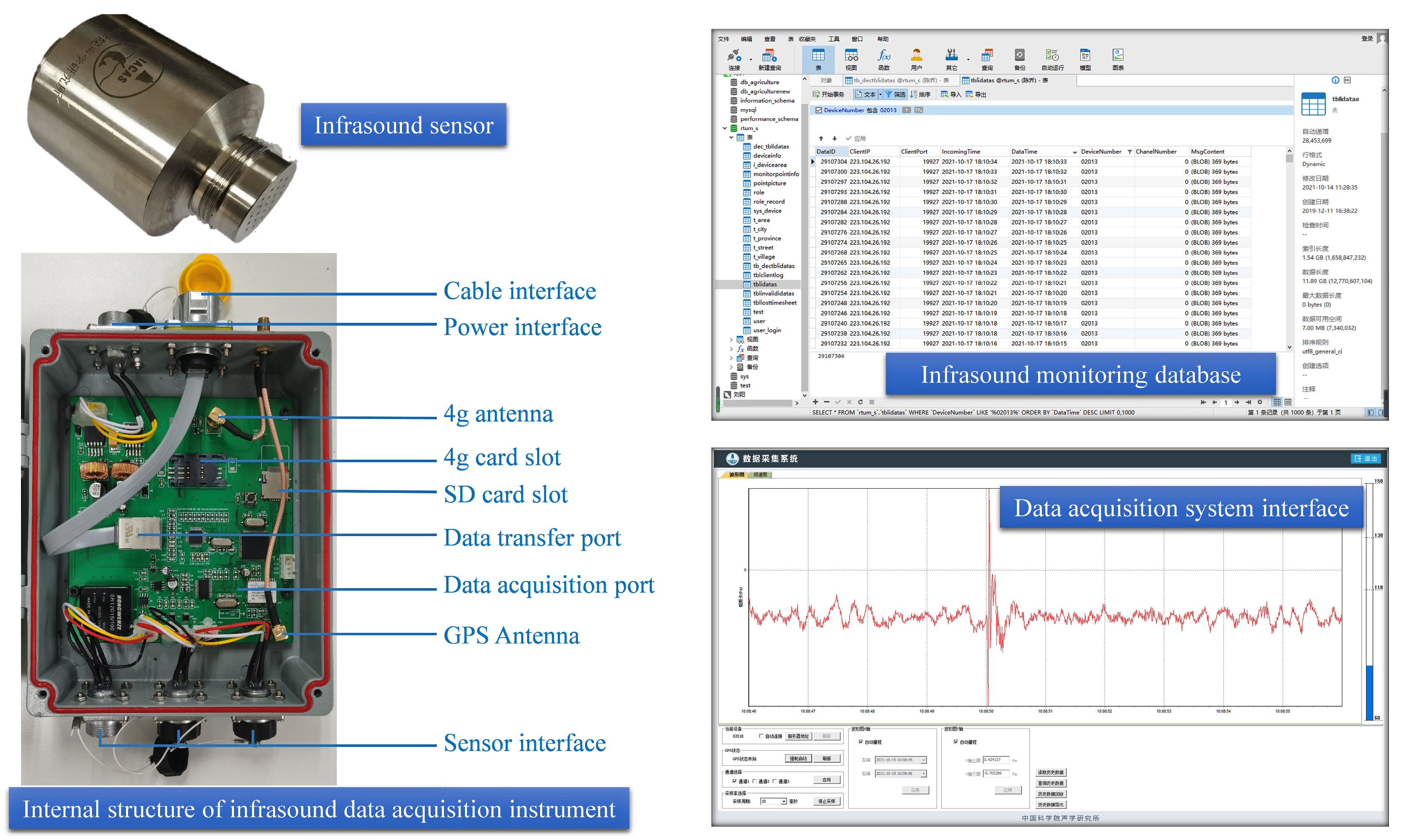
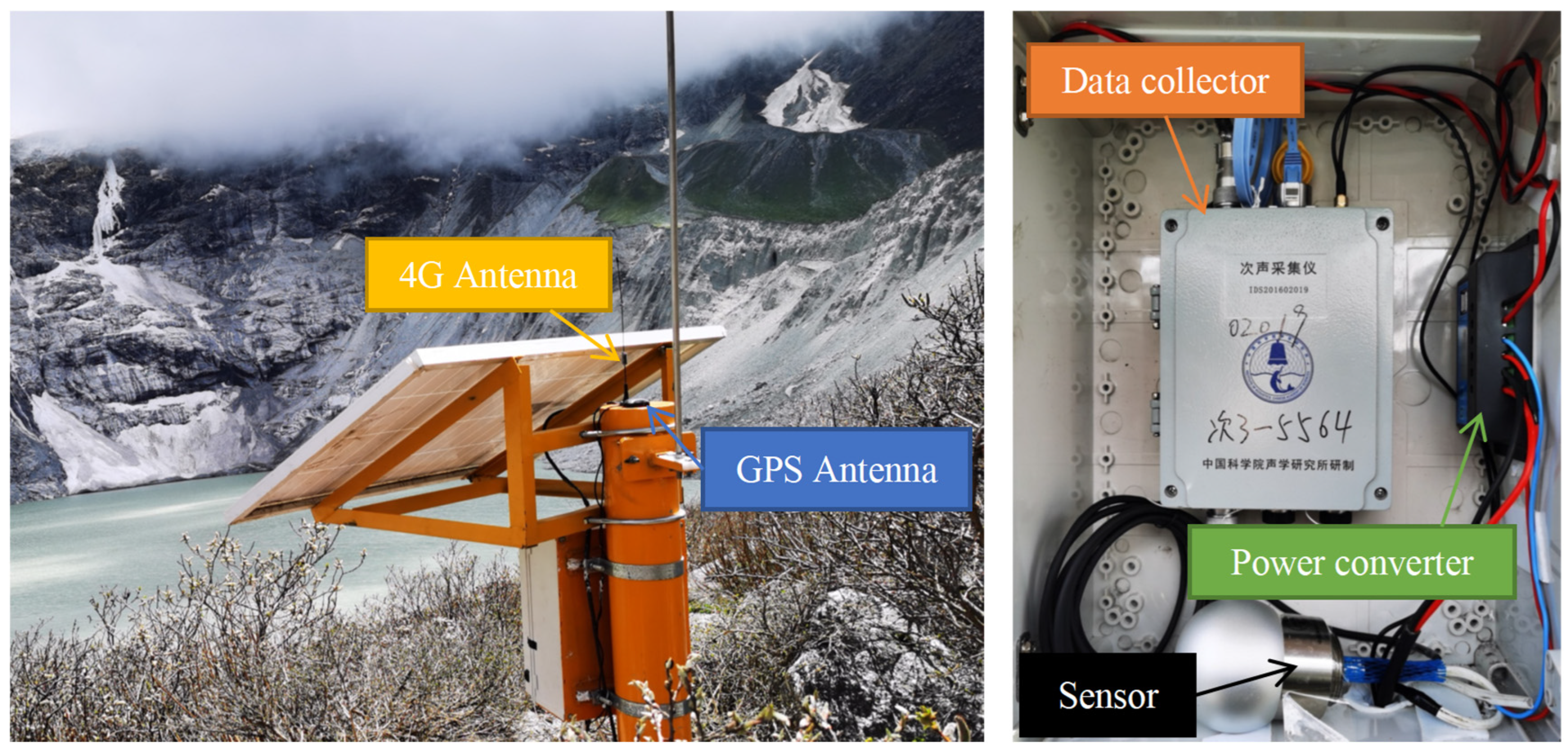
The infrasound monitoring equipment used in this study includes an infrasound sensor, infrasound data acquisition instrument, and supporting infrasound data acquisition system developed by the Institute of Acoustics, Chinese Academy of Sciences. The detectable range of the infrasound sensor is from 0.5 to 200 Hz. Its 50 mV/Pa sensitivity enables it to collect weak signals. Other indicators of the sensor are shown in

Table 2. Index parameters of infrasound sensor.

Index	Parameters
Type	IDS2016
Working voltage	±15 V
Working electricity	50 mA
Response amplitude	±10 V
Response frequency	0.1~1000 Hz
Sensitivity	50 mV/Pa

. The collected data are sent to the original infrasound database through a 4G network online (Figure 6).

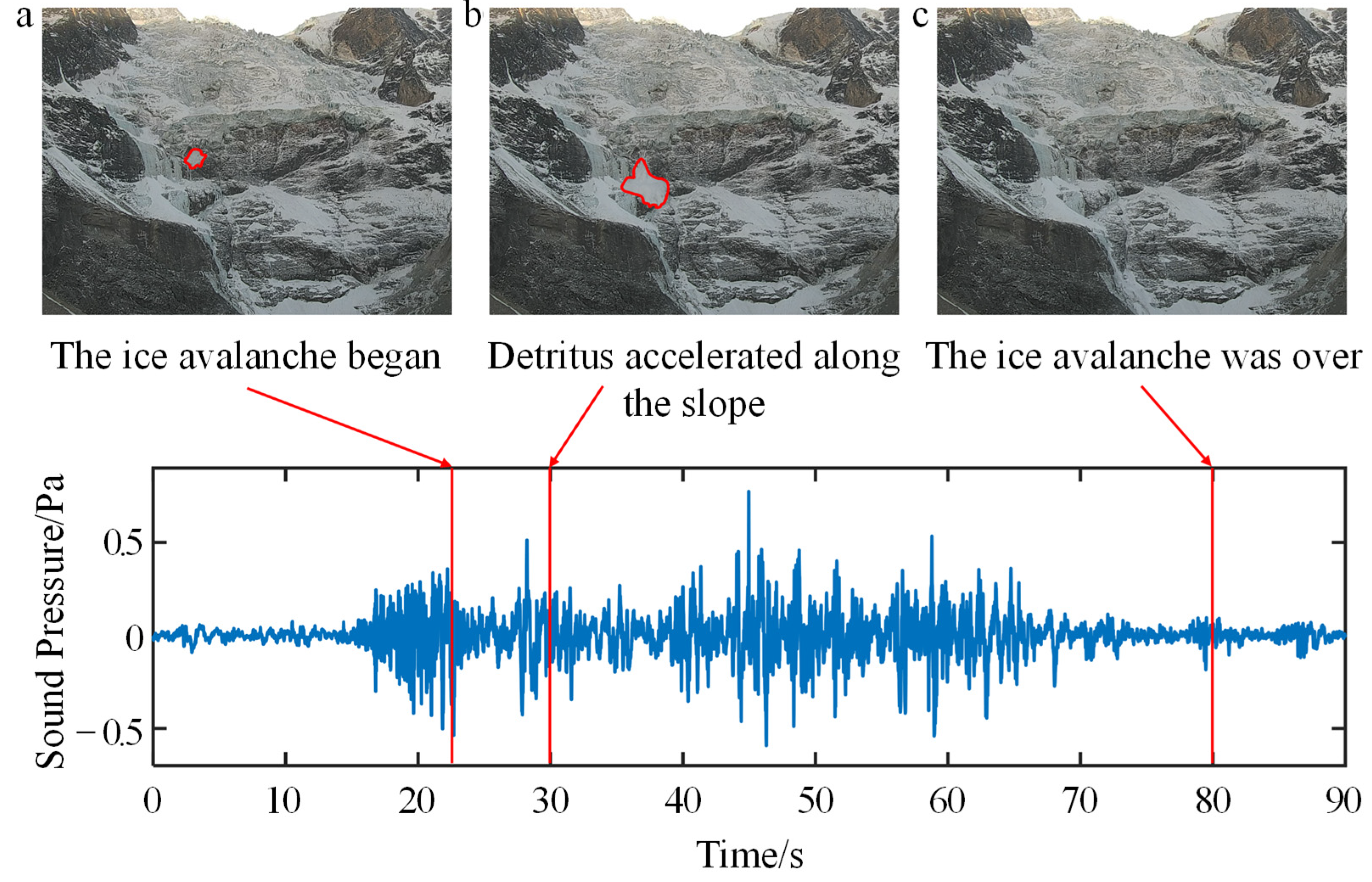
Since it is impossible to tell accurately that abnormal events monitored are ice avalanche events, a video surveillance device is installed near the infrasound array to realize video online transmission and local storage at the same time (see Figure 7 and Figure 8). In this study, infrasound signals occurring 2–3 min before and after a possible ice avalanche were collected and compared with the surveillance video to determine whether it was an ice avalanche event (see Figure 9).

2.3. Analysis Method

The collected signal needs to be processed before it can be analyzed. Figure 10 shows the signal processing work flow.

2.3.1. Infrasound Signal Preprocessing

The collected infrasound signals are discrete nonlinear data. Meanwhile, due to the insufficient power supply of the equipment and interruption of the network signal at the monitoring site, the collected infrasound signals may have some missing, high-frequency noise interference and a large amount of useless information, etc., so it is necessary to preprocess the original signals before extracting the features of the infrasound signals of ice avalanche, flood, wind, and rain events. The preprocessing aims to improve the signal-to-noise ratio of the signals through event sample extraction, de-DC (direct current) drift, and filtering.

(1)

Event sample extraction

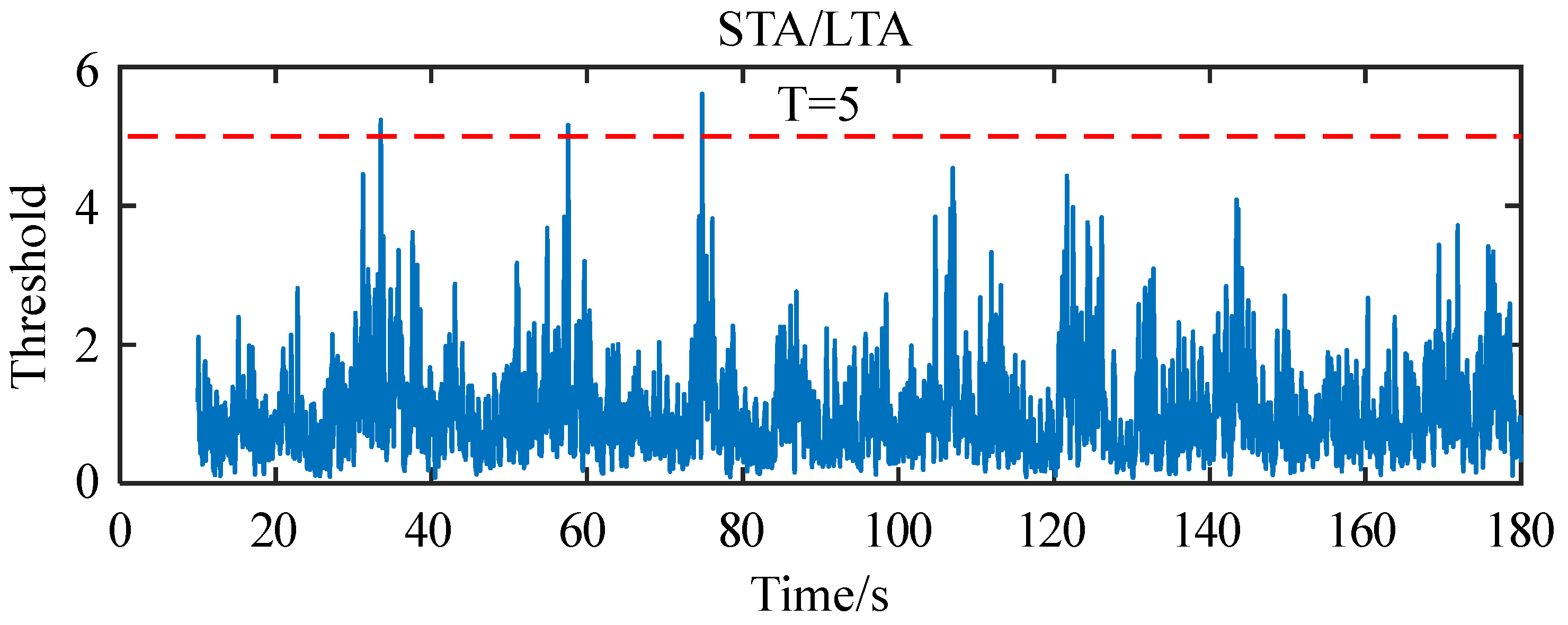
Due to the large amount of data and the traditional manual identification of samples taking a lot of time, the ratio of the short time average (STA) to the long time average (LTA), namely, the $STA/LTA$ time window ratio method, was used to obtain the first arrival time of events and judge if the events were an ice avalanche according to the first arrival time and the video surveillance. Then, the ice avalanche event samples were extracted.

The $STA/LTA$ time–window ratio method sets a long-time window and a short-time window, the windows move with the time series, and all signal amplitudes in the long-time window and short-time window are averaged at the same time. When the ratio R of the two windows exceeds the set threshold T, it is confirmed an event happened [26,27].

$$R=\frac{STA\left(i\right)}{LTA\left(i\right)}=\frac{W_{lta}{{\displaystyle \sum }}_{i=1}^{W_{sta}}\left|A\left(i\right)\right|}{W_{sta}{{\displaystyle \sum }}_{i=1}^{W_{lta}}\left|A\left(i\right)\right|}$$

(1)

In Equation (1), $W_{lta} \mathrm{and} W_{sta}$ are the lengths of the long-time window and short-time window, respectively, and $A\left(i\right)$ is the amplitude of the signal. In this study, the lengths of the long-time window and short-time window were 10 s and 0.1 s, respectively, and the threshold was set at 5. Figure 11 shows the identified avalanche events.

(2)

De-DC drift

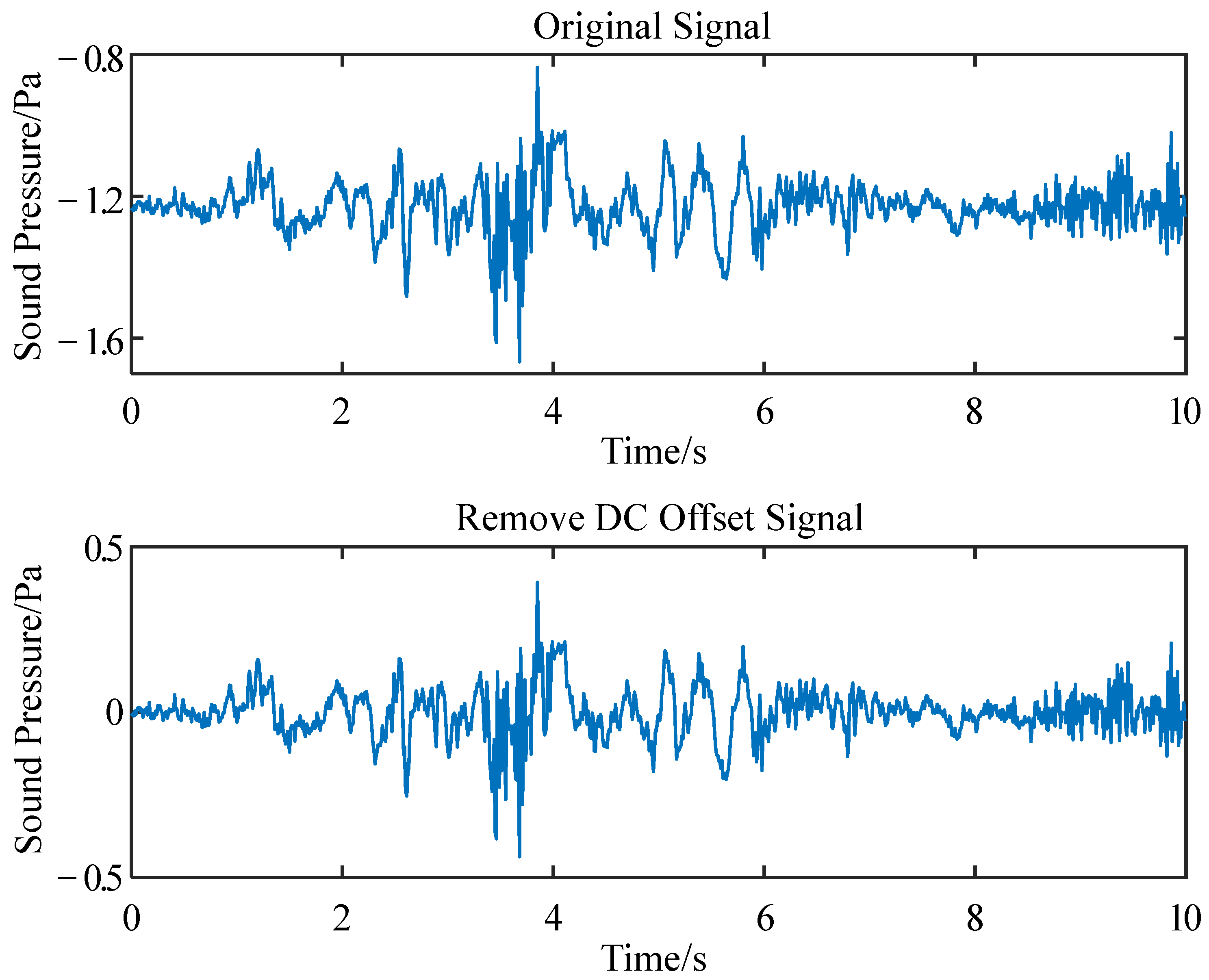
The data acquisition equipment can produce a constant interference signal during operation, namely, the DC component. This part of the signal does not carry information, but carries energy, which will convey an energy error to the subsequent data processing; so, it is necessary to remove it before signal processing.

$$y_{DC}\left(i\right)=y\left(i\right)-mean\left[y\left(i\right)\right]$$

(2)

where $y\left(i\right)$ is the original signal fragment containing the ice avalanche event for about 3 min. As shown in Figure 12, the original signal has a DC drift of about −1.2/Pa.

(3)

Filtering

The response frequency range of the infrasound sensor is 0.1–1000 Hz, that is, in the actual signal acquisition, part of the signals collected by the sensor will be greater than 20 Hz in frequency. As only the signals no more than 20 Hz in frequency were analyzed in this study, signals larger than 20 Hz in frequency need to be removed through filtering. The filter adopted the window function design method and, specifically, the Kaiser window with high adaptability. The filtering effect is shown in Figure 13.

2.3.2. Extraction Methods of Avalanche Infrasound Features

(1)

Extraction of time domain features

In this study, kurtosis and skewness of the signal are extracted to characterize the waveform characteristics of the signal in the time domain. Kurtosis reflects the gentle degree of the waveform: the higher the kurtosis, the steeper the waveform. Skewness reflects the deflection degree of the waveform: positive skewness indicates right skewness, negative skewness indicates left skewness.

Kurtosis is expressed as:

$$Ku=\frac{E{\left(x-\mu \right)}^4}{{\sigma }^4}$$

(3)

Skewness is expressed as:

$$Sk=\frac{E{\left(x-\mu \right)}^3}{{\sigma }^3}$$

(4)

In the equations above, $x$ represents the input signal, $\mu$ represents the mean value of the input signals, $\sigma$ represents the standard deviation of the input signal, and $E$ represents the expected value of the input signal.

(2)

Extraction of features in frequency domain

In this study, the frequency spectrum and power spectrum of the signal are obtained by Fast Fourier Transform (FFT), and the center of gravity frequency [28] and frequency standard deviation [29] of the signal are extracted. The center of gravity frequency represents the frequency distribution of the signal on the frequency spectrum. The frequency standard deviation characterizes the dispersion of the power spectrum energy of the signal.

$$X\left(f\right)=F\left[x\left(t\right)\right]={{\displaystyle \int }}_{-\infty }^{\infty }x\left(t\right)e^{-i2\pi ft}dt$$

(5)

$X\left(f\right)$ represents the Fourier transform of the signal, $f$ is the frequency, and $x\left(t\right)$ represents the input signal [30].

$$\widehat{P}=10\ast {\log }_{10}\frac{{\left|X\left(f\right)\right|}^2}{N}$$

(6)

$\widehat{P}$ is the power spectrum, $X\left(f\right)$ represents the fast Fourier transform of the signal, and $N$ represents the length of the signal.

$$FC=\frac{{{\displaystyle \int }}_0^{\infty }f\widehat{P}df}{{{\displaystyle \int }}_0^{\infty }\widehat{P}df}$$

(7)

$FC$ is the center of gravity frequency.

$$RVF=\sqrt{\frac{{{\displaystyle \int }}_0^{\infty }{\left(f-FC\right)}^2\widehat{P}df}{{{\displaystyle \int }}_0^{\infty }\widehat{P}df}}$$

(8)

$RVF$ is the standard deviation of the frequency.

(3)

Joint extraction of features in time and frequency domains

The time domain analysis and frequency domain analysis of the signal can only characterize the characteristics of the signal from one aspect. In this paper, wavelet and Hilbert–Huang transform analyses were selected to obtain wavelet coefficients and the Hilbert marginal spectrum distribution, respectively, which were used to characterize the features of the signal in both the time domain and the frequency domain.

① Wavelet transform

The discrete wavelet transform depends on the selection of the wavelet function, which is mainly divided into the following five steps [31]:

Step 1: suppose that the function $\psi \left(t\right)$ satisfies $\psi \left(t\right)\in L^2\left(R\right)$, and its Fourier transform $\widehat{\psi }\left(w\right)$ satisfies the following conditions, then $\psi \left(t\right)$ is a mother wavelet:

$$\underset{-\infty }{\overset{+\infty }{{\displaystyle \int }}}\frac{{\left|\hat{\psi }\left(w\right)\right|}^2}{\left|w\right|}dw<\infty$$

(9)

Step 2: by stretching and translating the mother wavelet, a set of wavelet basis functions ${\psi }_{a,b}\left(t\right)$ are obtained, such as the following formula, where $a,b\in R,a>0$, $a$ is the scale factor, and $b$ is the translation factor, all of which are continuously changing values:

$${\psi }_{a,b}\left(t\right)=\frac{1}{\sqrt{a}}\psi \left(\frac{t-b}{a}\right)$$

(10)

Step 3: the scale parameter a and the shift parameter b are discretized, that is, $a=2^j$, $b_{j,k}=2^{j}k$, $j,k\in Z$, and the discrete wavelet basis function, ${\psi }_{j,k}\left(t\right)$, is obtained, which is the wavelet coefficient $Coe\left(i_n\right)$:

$${\psi }_{j,k}\left(t\right)=\frac{1}{\sqrt{2^j}}\psi \left(\frac{\mathrm{t}}{2^j}-k\right)$$

(11)

Step 4: discrete wavelet transform of signal $x\left(t\right)$:

$$Wx\left(j,k\right)={{\displaystyle \int }}_{-\infty }^{+\infty }x\left(t\right){\psi }_{j,k}^{\ast }dt$$

(12)

Step 5: calculate the energy $E_i$ and energy proportion $P_i$ on different scales:

$$E_i=E_i\left(j,k\right)={{\displaystyle \sum }}_{k\in Z}{\left({\psi }_{j,k}\right)}^2$$

(13)

$$P_i==\frac{{\mathrm{E}}_i}{{{\displaystyle \sum }}_{i=1}^i{E}_i}$$

(14)

The main eigenvalue extracted based on the wavelet transform is the distribution value of wavelet coefficients, and the extraction includes four main steps:

Step 1: wavelet packet decomposition: the pre-processed signal is decomposed by three layers of wavelet packets, and the waveforms of 8 nodes can be obtained, and each node waveform corresponds to a set of wavelet packet coefficients $Coe\left(i_n\right)$.

Step 2: take the absolute values of the wavelet coefficients $Coe\left(i_n\right)$ of the waveform at each node and sum them.

$$S_w\left(i\right)={{\displaystyle \sum }}_{n=1}^n\left|Coe\left(i_n\right)\right|$$

(15)

where $n$ is a natural number of finite length of $1~n$.

Step 3: the ratio of the sum of wavelet packet coefficients of each node to the sum of all node coefficients is calculated:

$$R_w\left(i\right)=\frac{S_w\left(i\right)}{{{\displaystyle \sum }}_{i=1}^i{S}_w\left(i\right)}$$

(16)

where $i$ is the number of nodes corresponding to the number of decomposition layers, and in this study, the decomposition layers are three, that is, $i=2^3$.

Step 4: finally, the ratio of the ratio calculated in the above step and the ratio of the adjacent node is determined, and that is the eigenvalue of the wavelet coefficient distribution.

$$E{V}_w=\frac{R_w\left(i\right)}{R_w\left(i+1\right)} \left(i=1\dots i-1\right)$$

(17)

Through the above steps, the eigenvalues of the wavelet coefficient distribution corresponding to the signal can be extracted. In this study, the signal was decomposed by three layers of wavelet packets, and the corresponding eigenvalue dimension was the $2^3-1$ dimension.

② Hilbert–Huang transform

The main eigenvalues extracted based on the Hilbert–Huang transform are the Hilbert spectrum and Hilbert marginal spectrum. The marginal spectrum can reflect the distribution of signals at different frequencies, especially local characteristics of signals at lower frequencies. In this study, the proportions of different frequency segments corresponding to the Hilbert marginal spectrum were taken as the characteristics of different sample signals, that is, the frequency distribution value of the marginal spectrum [32,33].

The Hilbert–Huang transform is mainly divided into the following nine steps:

Step 1: find all the maximum points, minimum points, and endpoints of signal $x\left(t\right)$.

Step 2: the extreme points of all the marks in step 1 are interpolated, and then the upper and lower envelope sequences $E_{up}$ and $E_{low}$ of the signal $x\left(t\right)$ are obtained, and the mean value of the upper and lower envelope of signal $x\left(t\right)$ is calculated:

$$M_1\left(t\right)=\left(E_{\mathrm{up}}+E_{\mathrm{low}}\right)/2$$

(18)

Step 3: calculate the $IMF$ signal $I\left(t\right)$ of signal $x\left(t\right)$:

$$I_1\left(t\right)=x\left(t\right)-M_1\left(t\right)$$

(19)

Step 4: to judge whether $I\left(t\right)$ satisfies the two conditions of $IMF$, (1) the difference between the total number of cross-zero points of the signal waveform and the number of all extreme points is less than or equal to 1, (2) and the local mean of the upper and downer envelope of the signal is zero. If the above two conditions are satisfied, then $IM{F}_1=I_1\left(t\right)$, and the first $IMF$ component is obtained; if the condition is not satisfied, then steps 2 to 4 of the above are repeated as the signal until the two conditions of $IMF$ are met, and the $IM{F}_1$ is obtained.

Step 5: the $IM{F}_1$ component is removed to obtain the residual component $r_1$:

$$r_1=x\left(t\right)-IM{F}_1$$

(20)

Step 6: to judge whether $r_1$ conforms to the three conditions of EMD (Empirical Mode Decomposition), (1) if the number of extreme points of the signal is greater than or equal to 2, it means that there is at least one maximum and one minimum point; (2) the time scale of the extreme point can only determine the local time domain characteristics of the original signal; and (3) if a signal has no extreme point, there must be a singularity or inflection point that can be obtained by several differentials. If the above three conditions are satisfied, the EMD decomposition ends. If not, steps 2 to 5 above are repeated with $r_1$ as the new original signal to obtain other $IM{F}_n$ components.

Step 7: when $r_n$ satisfies the termination condition, the EMD decomposition ends, and the signal $x\left(t\right)$ can be expressed in the form of the sum of multiple $IMF$ components:

$$x\left(t\right)={{\displaystyle \sum }}_{i=1}^{n}IM{F}_i\left(t\right)+r_n\left(t\right) n\ge 1$$

(21)

Step 8: the Hilbert–Huang transform is performed on each $IMF$ component to obtain the Hilbert spectrum $H\left(w,t\right)$, where $Re$ represents the real part of the $IMF$ component:

$$H\left(w,t\right)=Re{{\displaystyle \sum }}_{i=1}^n{a}_i\left(t\right)e^{j{\theta }_i\left(t\right)}=Re{{\displaystyle \sum }}_{i=1}^n{a}_i\left(t\right)e^{j{{\displaystyle \int }}^{ }{w}_i\left(t\right)dt}$$

(22)

Step 9: the Hilbert spectrum $H\left(w,t\right)$ is integrated, and the marginal spectrum $h\left(w\right)$ is obtained:

$$h\left(w\right)={{\displaystyle \int }}_{-\infty }^{+\infty }H\left(w,t\right)dt$$

(23)

In this study, the proportion of different frequency segments corresponding to the Hilbert marginal spectrum is taken as the characteristic of different sample signals, that is, the marginal spectrum frequency distribution value. The extraction process mainly has the following four steps:

Step 1: the marginal spectrum of the signal is obtained by the Hilbert–Huang transform, and the marginal spectrum is divided according to 1 Hz. In this study, after resampling the original data, the corresponding sampling frequency is 25 Hz, so it can be divided into 25 frequency bands, each band corresponding to 1 Hz.

$$i=\frac{h\left(w\right)}{Fs}$$

(24)

$h\left(w\right)$ is the marginal spectrum, and $Fs$ is the sampling frequency.

Step 2: the sum of the marginal spectrums of each frequency band, that is, the sum of the amplitudes corresponding to the marginal spectrum, is determined as follows:

$$S_h\left(i\right)={{\displaystyle \sum }}_{n=1}^{n}A\left(i_n\right)$$

(25)

In the equation, $n$ is a finite natural number of $1~n$, and $A\left(i_n\right)$ is the amplitude corresponding to the marginal spectrum.

Step 3: the ratio of the sum of the marginal spectrums to the sum of the marginal spectrums corresponding to each frequency band is determined as follows:

$$R_h\left(i\right)=\frac{S_h\left(i\right)}{{{\displaystyle \sum }}_{i=1}^i{S}_h\left(i\right)},R_h\left(i\right)=\frac{S_h\left(i\right)}{{{\displaystyle \sum }}_1^{i\ast n}h\left(w\right)}$$

(26)

Step 4: finally, the ratio calculated in step 3 and the ratio of the adjacent frequency bands are calculated again, that is, the eigenvalue of the marginal spectral frequency distribution.

$$E{V}_h=\frac{R_h\left(i\right)}{R_h\left(i+1\right)} \left(i=1\dots i-1\right)$$

(27)

Through the above steps, the eigenvalues of the marginal spectrum frequency distribution corresponding to the signal can be extracted. In this study, 25 frequency segments are obtained after the marginal spectrum is segmented, and the corresponding eigenvalue dimension is 24 dimensions.

(4)

Extraction of information entropy feature

Information entropy is used to measure the uncertainty of random variables [34] (Zhu Xuenong, 2001), which is expressed as

$$H_p=-{{\displaystyle \sum }}_{n=1}^N{p}_n\log p_n$$

(28)

where $p_n$ represents the probability of occurrence of N values of the random variable.

In this study, eigenvalues extracted based on information entropy included singular spectrum entropy based on time domain analysis, power spectrum entropy based on frequency domain analysis, wavelet energy entropy based on the wavelet transform, wavelet packet energy entropy, wavelet packet scale entropy and wavelet packet singular entropy based on the wavelet packet transform, and energy entropy based on EMD(Empirical Mode Decomposition) decomposition.

① Singular spectral entropy based on time domain analysis

The singular spectrum of signals needs to be decomposed before solving the singular spectrum entropy, which includes decomposing and reconstructing signals according to the time series of the signals to extract different components of the signals [35].

$$X=U_{m\times m}{\Sigma }_{m\times n}{V}_{n\times n}{}^T$$

(29)

where $X$ denotes the $m\times n$ matrix of signals to be decomposed. $U$ is the unitary matrix of $m\times m$; $V$ is the unitary matrix of $n\times n$, that is, $U^{T}U=I$, $V^{T}V=I$; and $\Sigma$ is the matrix of $m\times n$.

It can be obtained from Equation (29).

$$XV=U\Sigma$$

(30)

$$X{\nu }_i={\mu }_i{\sigma }_i$$

(31)

where ${\nu }_i$ is the eigenvector of $X^{T}X$, ${\mu }_i$ is the eigenvector of $X{X}^T$, ${\sigma }_i$ are singular values.

$${\sigma }_i=\frac{X{\nu }_i}{{\mu }_i}$$

(32)

$$S_j={{\displaystyle \sum }}_{i=1}^n{\sigma }_i$$

(33)

The corresponding singular spectrum $S_j$ can be obtained by singular value decomposition of $X$. By calculating the proportion of every singular value in the singular spectrum, a set of probability density functions can be obtained. By substituting the probability density function into the classical entropy formula, the singular spectrum entropy of the input signal can be obtained.

$$p_j=\frac{S_j}{{{\displaystyle \sum }}_{j=1}^N{S}_j}$$

(34)

$$SV{D}_p=-{{\displaystyle \sum }}_{j=1}^N{p}_j\log p_j$$

(35)

② Power spectral entropy based on frequency domain analysis

In the part of the extraction of features in the frequency domain, the power spectrum of the input signal, $\widehat{P}$, has been obtained, and the power spectrum, $\widehat{P},$ contains $r$ band values. By calculating the proportion of every band value of the power spectrum ${\widehat{P}}_r$ in the power spectrum, a set of probability density functions $p_r$ can be obtained. The power spectrum entropy of the input signal can be obtained by substituting the probability density function into the classical entropy formula.

$$p_r=\frac{{\widehat{P}}_r}{{{\displaystyle \sum }}_{r=1}^N{\widehat{P}}_r}$$

(36)

$$PS{D}_p=-{{\displaystyle \sum }}_{r=1}^N{p}_r\log p_r$$

(37)

③ Wavelet energy entropy and wavelet packet energy entropy based on the wavelet and wavelet packet transforms

In the part of the extraction of features through the wavelet and wavelet packet transforms, the energy $E_i$ and energy proportion $P_i$ of each layer after wavelet decomposition have been calculated, and then the energy entropy can be determined.

$$p_i=\frac{E_i}{{{\displaystyle \sum }}_{i=1}^N{E}_i}$$

(38)

$$E_p=-{{\displaystyle \sum }}_{i=1}^N{p}_i\log p_i$$

(39)

④ Wavelet packet scale entropy and wavelet packet singular entropy based on the wavelet packet transform

Similarly, the wavelet scale entropy is the Shannon entropy of the probability density of the wavelet coefficients $Co{e}_k$ of all nodes in the wavelet packet decomposition.

$$p_k=\frac{Co{e}_k}{{{\displaystyle \sum }}_{k=1}^{N}Co{e}_k}$$

(40)

$$S{E}_p=-{{\displaystyle \sum }}_{k=1}^N{p}_k\log p_k$$

(41)

The calculation method of singular entropy of the wavelet packet is consistent with that of singular spectral entropy of the input signal, that is, the singular value of each node $S_j$ is obtained by singular spectral decomposition of the wavelet packet coefficients of each node, and then the singular entropy of wavelet packet $SV{D}_p$ is obtained by the same method.

⑤ Energy entropy based on EMD decomposition

In the part of the extraction of features through the Hilbert–Huang transform, a set of IMF (Intrinsic Mode Function) components of the input signal $im{f}_s$ can be obtained by EMD decomposition, and the energy entropy of the probability density function $p_j$ corresponding to each group of $im{f}_j$ can be obtained.

$$p_s=\frac{im{f}_s}{{{\displaystyle \sum }}_{s=1}^{N}im{f}_s}$$

(42)

$$EM{D}_p=-{{\displaystyle \sum }}_{s=1}^N{p}_s\log p_s$$

(43)

The eigenvalues of ice avalanche events, flood events, and wind-and-rain events extracted by using the above feature extraction methods constitute feature vectors of different features.

2.3.3. Class Recognition Method

In this study, supervised pattern recognition was used to classify infrasound signals. Support vector machine (SVM), K-nearest neighbor (KNN), classification tree, and BP neural network (BPNN) were used. After preprocessing of the original infrasound signals, based on feature vectors extracted by time and frequency domain analysis, the wavelet transform and the Hilbert–Huang transform, classification models were constructed, and the model parameters were improved through continuous training to achieve the best classification effect. The trained classification models have been applied to the recognition of unknown signals to judge classes of the signals, with the classification results output [36,37].

In order to characterize the recognition effect of the models more accurately, five indexes—recall ratio, precision, accuracy, F1 score, and area under the curve (AUC) were used to evaluate the classification results of the models.

The recall ratio, also known as recall, refers to the ratio of samples of a class identified in the process of class recognition to the actual total samples of this class. It is generally considered that the higher the value, the better the performance of the classifier is, but the higher recall rate also means a greater possibility of misjudgment.

$$Re=\frac{TP}{TP+FN}\ast 100\%$$

(44)

$TP$ refers to the number of samples of the class concerned that are true in the actual situation and prediction, while $FN$ is the number of samples that are true, but predicted as false.

Precision refers to the ratio of the actual samples to the predicted samples of the concerned class in the process of class recognition. The higher the value, the better the performance of the classifier is.

$$Pr=\frac{TP}{TP+FP}\ast 100\%$$

(45)

$FP$ represents the number of samples of the class in concern that are actually false, but predicted as true.

Accuracy refers to the ratio of the correctly predicted events to the total events, which characterizes the performance of the classifier. And, the higher the value, the better the classifier is.

$$Ac=\frac{TP+TN}{TP+TN+FP+FN}\ast 100\%$$

(46)

$TN$ indicates the number of samples that are false in the actual situation and prediction.

The $F1$ score can characterize the recall rate and accuracy rate at the same time, and it is the harmonic average that can maintain the two indexes as high at the same time.

$$F1=2\ast \frac{Re\ast Pr}{\left(Re+Pr\right)}$$

(47)

The area under the, AUC, refers to the area under the Receiver Operating Characteristic Curve (ROC). Its abscissa is the false positive rate; its vertical coordinate is the true positive rate, in which the true positive rate is equal to the recall rate; and the closer the curve is to the upper left corner, the better the recognition effect is. In order to quantitatively characterize the performance of the classifier, AUC, that is, the area under the ROC, values ranging from 0 to 1 are introduced. The closer the AUC value is to 1, the better the performance of the model.

As the main purpose of class identification is to identify disaster events, and this study focuses on ice avalanche disasters, the three types of events were given different weights, ice avalanche events 0.5, flood events 0.4, wind-and-rain events 0.1, and the comprehensive index of each classification model was calculated.

3. Results and Discussion

3.1. Characteristic Response Analysis of Avalanche Infrasound

As only a small number of ice avalanche events have been monitored so far, the recognition effect may not be obvious or ideal due to insufficient training samples in the later class recognition of ice avalanche signals. Therefore, the captured six complete ice avalanche events (about 3 min of each event) were divided into 151 short-time-series ice avalanche events and combined with 386 samples of wind-and-rain events and 146 samples of flood events, and the classifiers were trained to improve the effect of class identification of ice avalanche events. The infrasound signal data of the three types of events used for subsequent class identification in this paper all come from the infrasound monitoring equipment installed by us. By using the above feature extraction methods, characteristic responses of different events in waveform, sound pressure, power spectrum, and frequency distribution have been obtained, as shown in

Table 3. Characteristics of different events in time domain and frequency domain.

	Feature	Kurtosis		Skewness		Sound Pressure Peak/Pa		Average Power Spectrum/dB
Event		Value	Variance	Value	Variance	Value	Variance	Value	Variance
Ice avalanche		5.67	7.85	−0.09	0.23	2.83	7.76	−41.48	56.72
Flood		8.33	6.91	−0.13	0.10	331.80	12,214.11	−2.35	6.71
Wind and rain		6.90	7.46	−0.16	0.27	4.62	10.94	−37.83	61.43
Background		3.81	0.16	0.00	0.01	0.10	0.00	−69.56	25.25

and

Table 4. Wavelet frequency distribution characteristics of different events.

	Frequency Range/Hz	0–0.79		0.79–1.57		1.57–3.13		3.13–6.25		6.25–12.5		12.5–25
Event		Value	Variance	Value	Variance	Value	Variance	Value	Variance	Value	Variance	Value	Variance
Ice avalanche		7.45	32.29	14.72	79.94	23.79	95.80	24.17	87.66	19.75	157.34	10.11	157.26
Flood		0.31	0.02	1.05	0.16	7.18	2.71	27.29	10.78	41.90	10.51	22.27	6.40
Wind and rain		10.01	27.18	22.03	74.42	30.98	75.02	21.14	47.49	10.76	28.17	5.08	6.02
Background		3.32	3.27	2.42	7.18	4.10	6.65	24.61	12.66	48.39	24.85	17.16	35.19

.

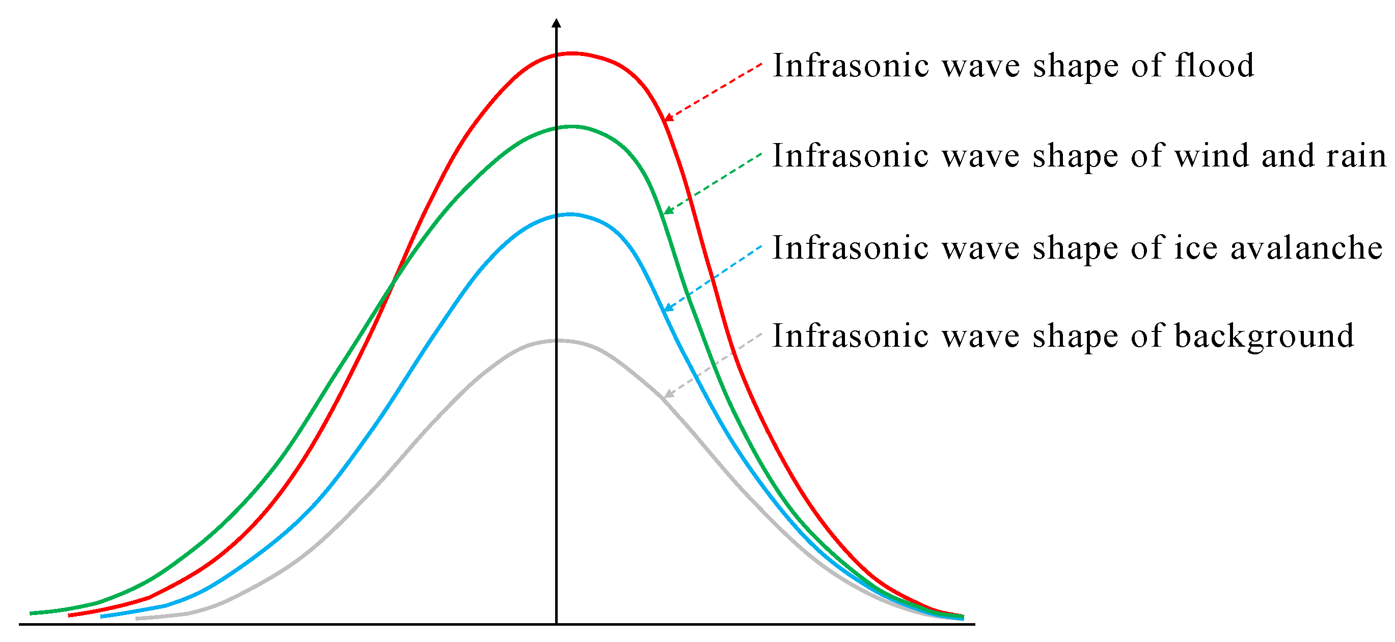
Different kinds of events have some differences in waveform. Figure 14 is a schematic diagram of the waveform based on the kurtosis and skewness in Table 3. As shown in Figure 14, the gray curve in the figure is the waveform feature of background noise, which basically shows a standard normal distribution, and the waveform of the flood event (red curve in the figure) has the maximum kurtosis of 8.33; therefore, it is steeper than those of other events and has a skewness of −0.13, that is, showing a left trailing phenomenon, which is slightly slighter than that of wind-and-rain events (green curve in the picture). The waveform of wind-and-rain events has a skewness of −0.16 and shows a more obvious characteristic of left trailing among the three kinds of events. In comparison, the waveform of the ice avalanche event has kurtosis and skewness (the blue part in the figure) less obvious than those of the other two kinds of events. In addition, there are overlaps between the three kinds of events and background noise in frequency range, which makes it difficult to remove the background noise. But, the background noise is very small in sound pressure and has little impact on the events. Therefore, there was no specific processing to remove the background noise in this study.

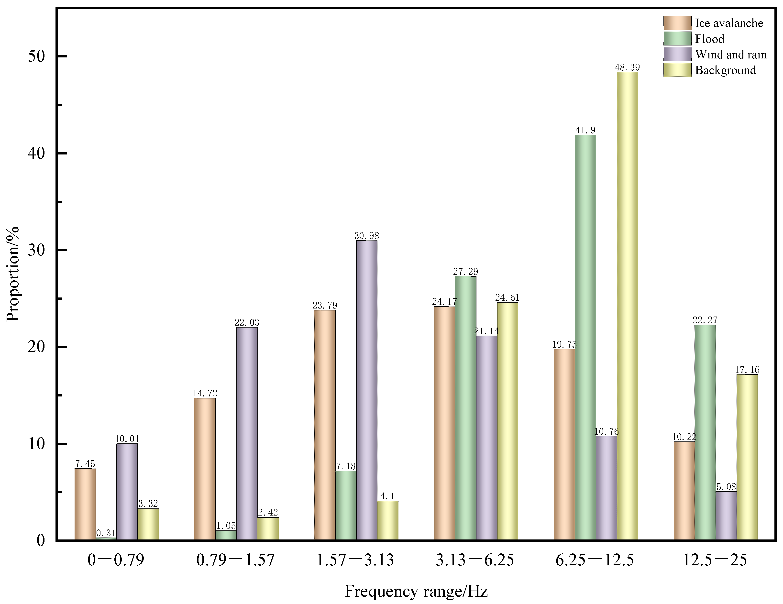
In terms of frequency distribution characteristics, avalanche events, flood events, and wind-and-rain events are mainly distributed in the frequency ranges of 1.5–9.5 Hz, 3–12.5 Hz, and 0.5–6.5 Hz, respectively, while background noise is mainly concentrated in the frequency range of 3–12.5 Hz. As shown in Figure 15, these events have certain overlaps among each other and overlaps with background noise, but they also differ some in frequency characteristics.

3.2. Class Recognition of Avalanche Infrasound

Through pre-processing and feature extraction of the three kinds of events, the features of different events were extracted in a total of 63 dimensions, including 4 dimensions in the time domain and the frequency domain, 7 dimensions extracted by the wavelet transform (distribution values of wavelet coefficients), 24 dimensions extracted by the Hilbert–Huang transform (frequency distribution value of marginal spectrum), and 14 dimensions of information entropy. The information entropy features are subdivided into seven dimensions of total entropy (total entropy) and seven dimensions of partial entropy (the partial entropy is only the information entropy of part of the components). As shown in

Table 5. Eigenvalue categories and corresponding dimensions.

Method	Total Dimension	Eigenvalue	Dimension
Time–Frequency	4	Kurtosis	1
		Skewness	1
		Center of gravity frequency	1
		Frequency standard deviation	1
Wavelet packet transform	7	Wavelet coefficient distribution	7
Hilbert–Huang transform	24	Marginal spectral frequency distribution	24
Information entropy	7	Singular spectral entropy based on time domain	1
		Power spectral entropy based on frequency domain	1
		Wavelet energy entropy (Total information entropy)	1
		Wavelet packet energy entropy (Total information entropy)	1
		Wavelet packet-scale entropy (Total information entropy)	1
		Wavelet packet singular entropy (Total information entropy)	1
		Energy entropy based on EMD decomposition	1
	7	Wavelet energy entropy (Partial information entropy)	1
		Wavelet packet energy entropy (Partial information entropy)	2
		Wavelet packet-scale entropy (Partial information entropy)	2
		Wavelet packet singular entropy (Partial information entropy)	2

, there are great differences between the extracted different eigenvalues, so each type of feature extracted should be standardized to obtain the standard input data type for the class recognition.

Table 6. Comparison of recall rates of four kinds of models.

	Feature Type	Time–Frequency	Information Entropy	Partial Information Entropy	Total Information Entropy	Wavelet Coefficient Distribution	Marginal Spectral Frequency Distribution
Model
Support vector machine		66.6	99.4	91.3	91.3	88.0	99.1
K-nearest neighbor		68.2	99.2	91.5	89.6	82.4	93.0
Classification tree		63.9	90.3	82.5	81.9	82.8	97.7
BP neural network		70.2	99.7	85.9	90.4	93.1	99.7

,

Table 7. Comparison of accuracy values of the four kinds of models.

	Feature Type	Time–Frequency	Information Entropy	Partial Information Entropy	Total Information Entropy	Wavelet Coefficient Distribution	Marginal Spectral Frequency Distribution
Model
Support vector machine		83.1	99.7	96.6	95.1	93.8	97.4
K-nearest neighbor		87.0	99.0	94.4	92.7	92.5	98.5
Classification tree		79.6	93.7	88.0	87.1	90.0	98.0
BP neural network		81.7	99.7	90.5	91.4	95.0	100.0

,

Table 8. Comparison of F1 scores of the four kinds of models.

	Feature Type	Time–Frequency	Information Entropy	Partial Information Entropy	Total Information Entropy	Wavelet Coefficient Distribution	Marginal Spectral Frequency Distribution
Model
Support vector machine		73.1	99.5	93.7	93.1	90.5	98.3
K-nearest neighbor		75.3	99.1	92.9	91.1	86.1	95.5
Classification tree		70.1	91.9	85.0	84.3	85.6	97.8
BP neural network		75.2	99.6	88.1	90.9	94.0	99.8

,

Table 9. Comparison of AUC indicators of the four kinds of models.

	Feature Type	Time–Frequency	Information Entropy	Partial Information Entropy	Total Information Entropy	Wavelet Coefficient Distribution	Marginal Spectral Frequency Distribution
Model
Support vector machine		0.89	1.00	0.99	0.99	0.98	1.00
K-nearest neighbor		0.89	0.99	0.99	0.98	0.95	1.00
Classification tree		0.80	0.94	0.91	0.91	0.91	0.99
BP neural network		0.90	1.00	0.98	0.98	0.99	0.96

and

Table 10. Comparison of precision of the four kinds of models.

	Feature Type	Time–Frequency	Information Entropy	Partial Information Entropy	Total Information Entropy	Wavelet Coefficient Distribution	Marginal Spectral Frequency Distribution
Model
Support vector machine		78.5	99.7	95.0	93.1	90.2	96.9
K-nearest neighbor		81.4	98.7	94.4	90.6	88.0	96.6
Classification tree		75.4	93.3	87.6	85.1	84.9	98.5
BP neural network		81.8	99.9	91.4	92.8	94.6	99.8

list the recall rate, accuracy values, F1 score, AUC, and precision of the four kinds of algorithm models.

It can be seen from Table 6, in terms of the recall rate, support vector machine, K-nearest neighbor algorithm, and classification tree algorithm, that models based on the time–frequency feature have a poor class recognition effect, while BP neural network algorithm models yield average class recognition results, and the four algorithm models based on information entropy and marginal spectral frequency distribution all have a very good classification effect. The support vector machine and K-nearest neighbor algorithm based on partial information entropy have a very good classification effect, while the classification tree and BP neural network models based on partial information entropy have a fairly good classification effect. The support vector machine and BP neural network model based on total information entropy have a very good classification effect; the K-nearest neighbor algorithm and classification tree based on total information entropy have a fairly good classification effect; and the BP neural network based on wavelet coefficient distribution has a very good classification effect, while the other three algorithm models based on this feature have a fairly good classification effect.

It can be seen from Table 7 that the classification tree algorithm model based on the time–frequency feature has an average class recognition effect, and the other three algorithm models based on this feature have a fairly good class recognition effect. The four algorithm models based on information entropy, the wavelet coefficient distribution, and the marginal spectral frequency distribution have a very good classification effect. The classification tree models based on partial information entropy and total information entropy have a fairly good classification effect, and the other three algorithms based on these features have a very good classification effect. Generally speaking, the classification tree algorithm has a poorer classification effect than the other three classification algorithms in terms of accuracy.

It can be seen from Table 8 that the four algorithm models based on time–frequency features are average in the class recognition effect; the four algorithm models based on information entropy and marginal spectral frequency distribution features all have very good class recognition results; the support vector algorithm models based on the other features, except time–frequency features, have the best class recognition effect; and although the classification tree algorithm model has a fairly good class recognition effect, it is still dead last among the four models.

It can be seen from Table 9 that, except for the classification tree algorithm model (with a fairly good class recognition effect), all the other three kinds of algorithm models have AUC indexes higher than 0.95. That is to say, they have a very good class recognition effect. Similarly, the models based on time–frequency features have a poorer class recognition effect; except for the classification tree model with an average class recognition effect, the other three kinds of models based on time–frequency features have a fairly good class recognition effect.

It can be seen from Table 10 that the precision of the BP neural network model is the best, while classification tree is the worst, and the precision based on time–frequency features is still the lowest. To sum up, all four kinds of models based on time–frequency features have a poorer class recognition effect (average) than those based on other features; the four kinds of algorithm models based on marginal spectral frequency distribution features all have a very good class recognition effect; the classification tree model based on information entropy has a fairly good class recognition effect; and the other models based on information entropy have a fairly good class recognition effect. The support vector machine model based on partial information entropy has a very good class recognition effect, while the other models based on this feature have a fairly good class recognition effect. The four kinds of models based on the total information entropy and distribution characteristics of wavelet coefficients all have a fairly good class recognition effect. The class recognition effects of the models are closely related to the differences between the selected features, and the models based on information entropy and marginal spectral frequency distribution features with the best classification effect characterize more details of the original signals. Among the four kinds of models, the support vector machine and BP neural network models are roughly the same in class recognition effect. BP neural network models are slightly better than support vector machine models, and K-nearest neighbor algorithm models take the third place. The classification tree models have the poorest effect among the four kinds of models, but they still have a fairly good effect in recognizing events by class.

Therefore, in practical application, it is not recommended to train models to recognize events based on time–frequency features alone; but, time–frequency features can be combined with other features to form recognition features of higher dimensions. Information entropy features and marginal spectral frequency distribution features can better reflect the subtle differences among different infrasound signals, so they can be used as recognition features for subsequent class recognition training. The four kinds of class recognition algorithms all have fairly good recognition results in this study, but the infrasound samples of disasters are often few in number and uneven in distribution, so the K-nearest neighbor and classification tree algorithms are likely to have large errors in this circumstance.

4. Conclusions and Future Prospects

The main results are as follows:

(1) The waveform of background noise basically shows a standard normal distribution; avalanche events are steeper than background noise and show slight left skewness in the waveform; wind-and-rain events have more left skewness in the waveform than ice avalanche events and flood events; and flood events are steeper than the other events in the waveform, showing obvious impact characteristics.

(2) In terms of frequency distribution, the ice avalanche events, flood events, wind-and-rain events, and background noise are distributed in the frequency ranges of 1.5–9.5 Hz, 3–12.5 Hz, 0.5–6.5 Hz, and 3–12.5 Hz, respectively. These events have a certain overlap in frequency, but some different characteristics. For the background noise and flood events with the same frequency range, in the same frequency distribution range, the frequency distribution of flood events decreases gradually with the increase in frequency, while the frequency distribution of background noise increases at first and then decreases with the increase in frequency, reaching a peak distribution value between 6.0 and 9.5 Hz.

(3) The BP neural network is similar to the support vector machine algorithm in class recognition effect. The BP neural network is slightly better than the support vector machine algorithm, followed by the K-nearest neighbor algorithm, and the classification tree algorithm is dead last in class recognition effect, so it is suggested the support vector machine or BP neural network algorithm be used to recognize ice avalanche infrasound events.

Some research prospects are as follows:

(1) Carry out indoor ice avalanche tests. As there are few ice avalanches actually monitored, the conclusions of this study may not be universal. Therefore, the indoor test of ice avalanches needs to be performed. By monitoring the infrasound signal of a glacier fracture under different variables, the early warning model of ice avalanches will be established to further improve the accuracy of field monitoring.

(2) Construction of more ice avalanche infrasound monitoring arrays. Glaciers are widely distributed in the Qinghai–Tibet Plateau, global warming has led to the decline of glacier stability, and there are serious security risks. Infrasound has the characteristics of long propagation distance and low attenuation. With the further deepening of research work, we will deploy more infrasound arrays and a video surveillance system in the research area for monitoring, which can collect a more effective and larger number of ice avalanche infrasound event samples for the training of artificial intelligence infrasound signal recognition models in this study. At the same time, as the number of infrasound sensors in the infrasound array increases, it will also lay the foundation for further improving the accuracy of infrasound positioning of the location of ice avalanche events. By strengthening the construction of avalanche infrasound monitoring arrays, ice avalanche events can be monitored and located remotely. And, we can lay the foundation for the follow-up early warning of an ice avalanche disaster and disaster chain.

References

1. Hu, W.; Yao, T.; Yu, W.; Yang, W.; Gao, Y. Advances in the study of glacier avalanches in High Aisa. J. Glaciol. Geocryol. 2018, 40, 1141–1152. [Google Scholar]
2. Pei, L. The Preliminary Study of Characteristics and Types of Ice Avalanche Disaster in the Tibetan Plateau. Master’s Thesis, China University of Geosciences, Beijing, China, 2019. [Google Scholar]
3. Tong, L.; Pei, L.; Tu, J.; Guo, Z.; Yu, J.; Fan, J.; Li, D. A preliminary study of definition and classification of ice avalanche in the Tibetan Plateau region. Remote Sens. Land Resour. 2020, 32, 11–18. [Google Scholar]
4. Wang, S.; Wen, J. Characteristics, influence of cryosphere disaster and prospect of discipline development. Bull. Chin. Acad. Sci. 2020, 35, 523–530. [Google Scholar]
5. Cui, P.; Guo, X.; Jiang, T.; Zhang, G.; Jin, W. Disaster effect induced by Asian Water Tower change and mitigation strategies. Bull. Chin. Acad. Sci. 2019, 34, 1313–1321. [Google Scholar]
6. Zhong, D.; Xie, H.; Wei, F.; Liu, H.; Tang, J. Discussion on mountain hazards chain. Mt. Res. 2013, 31, 314–326. [Google Scholar]
7. Huang, T. Spatial-Temporal Changes of Glacier Thickness and Lake Level on the Qinghai-Tibetan Plateau. Master’s Thesis, University of Chinese Academy of Sciences (Institute of Remote Sensing and Digital Earth Chinese Academy Sciences), Beijing, China, 2017. [Google Scholar]
8. Pinchak, A.C. Avalanche Activity on the Vaughan Lewis Icefall, Alaska. J. Glaciol. 1968, 7, 441–448. [Google Scholar] [CrossRef]
9. Hans, R. Ice Avalanches. J. Glaciol. 1977, 19, 669–671. [Google Scholar]
10. Margreth, S.; Funk, M. Hazard mapping for ice and combined snow/ice avalanches—Two case studies from the Swiss and Italian Alps. Cold Reg. Sci. Technol. 1999, 30, 159–173. [Google Scholar] [CrossRef]
11. Salzmann, N.; Kääb, A.; Huggel, C.; Allgöwer, B.; Haeberli, W. Assessment of the hazard potential of ice avalanches using remote sensing and GIS-modelling. Nor. Geogr. Tidsskr.-Nor. J. Geogr. 2004, 58, 74–84. [Google Scholar] [CrossRef]
12. Vilajosana, I.; Suriñach, E.; Khazaradze, G.; Gauer, P. Snow avalanche energy estimation from seismic signal analysis. Cold Reg. Sci. Technol. 2007, 49, 72–85. [Google Scholar] [CrossRef]
13. Herwijnen, A.V.; Schweizer, J. Monitoring avalanche activity using a seismic sensor. Cold Reg. Sci. Technol. 2011, 69, 165–176. [Google Scholar] [CrossRef]
14. Murayama, T.; Kanao, M.; Yamamoto, M.; Ishihara, Y. Infrasound Signals and Their Source Location Inferred from Array Deployment in the Lützow-Holm Bay Region, East Antarctica: January–June 2015. Int. J. Geoences 2017, 8, 181–188. [Google Scholar]
15. Asming, V.E.; Baranov, S.V.; Vinogradov, A.N.; Vinogradov, Y.A.; Fedorov, A. V Using an infrasonic method to monitor the destruction of glaciers in Arctic conditions. Acoust. Phys. 2016, 62, 583–592. [Google Scholar] [CrossRef]
16. Mayer, S.; van Herwijnen, A.; Ulivieri, G.; Schweizer, J. Evaluating the performance of an operational infrasound avalanche detection system at three locations in the Swiss Alps during two winter seasons. Cold Reg. Sci. Technol. 2020, 173, 102962. [Google Scholar] [CrossRef]
17. Graveline, M.H.; Germain, D. Ice-block fall and snow avalanche hazards in northern Gaspésie (eastern Canada): Triggering weather scenarios and process interactions. Cold Reg. Sci. Technol. 2016, 123, 81–90. [Google Scholar] [CrossRef]
18. Lv, R.; Li, D. Debris flow induced by ice lake burst in the Tangbulang Gully, Gongbujiangda, Xizang (Tibet). J. Glaciol. Geocryol. 1986, 8, 61–71. [Google Scholar]
19. Liu, J.; Cheng, Z.; Li, Y.; Su, P. Characteristics of Glacier-Lake Breaks in Tibet. J. Catastrophol. 2008, 23, 55–60. [Google Scholar]
20. Cheng, Z.; Zhu, P.; Dang, C.; Liu, J. Hazards of debris flow due to glacier-lake outburst in southeastern Tibet. J. Glaciol. Geocryol. 2008, 30, 954–959. [Google Scholar]
21. Yao, X.; Liu, S.; Sun, M.; Zhang, X. Study on the glacial lake outburst flood events in Tibet since the 20th century. J. Nat. Resour. 2014, 29, 1377–1390. [Google Scholar]
22. Zhang, J.; Pang, J.; Li, C. Physics properties of infrasonic waves and its applications. Phys. Bull. 2018, 123–126. [Google Scholar] [CrossRef]
23. Tong, N. Features and applications of infrasound. Tech. Acoust. 2003, 22, 199–202. [Google Scholar]
24. Zheng, F.; Chen, W.; Lin, C. Research status and progress of infrasound in disaster monitoring. Sci. Technol. Eng. 2015, 15, 129–137. [Google Scholar]
25. Shang, Y. Study on the Analysis Method of Infrasonic Signal. Master’s Thesis, Kunming University of Science and Technology, Kunming, China, 2013. [Google Scholar]
26. Hu, Z. Characteristics and Type Identification of Debris Flow Acoustic Signal. Master’s Thesis, University of Chinese Academy of Science (Institution of Mountain Hazards and Environment, Chinese Academy of Sciences), Chengdu, China, 2020. [Google Scholar]
27. Duan, J.; Cheng, J.; Wang, Y.; Lu, B.; Zhu, H. Automatic identification technology of microseismic event based on STA/LTA algorithm. Coal Geol. Explor. 2015, 43, 76–80+85. [Google Scholar]
28. Yang, J.; Zhang, D.; Lu, J.; Shuai, X. Gravity frequency and its monitoring application of EEG spectrum in the vigilance operation. J. Biomed. Eng. 2014, 31, 257–261. [Google Scholar]
29. Xing, N.; Liu, F.; Zhou, C.; Xu, L. Cutting chatter feature extraction method based on mean square frequency and empirical mode decomposition. Manuf. Technol. Mach. Tool 2021, 35–40. [Google Scholar] [CrossRef]
30. Zheng, J.; Ying, Q.; Yang, W. Signals and Systems, 3rd ed.; Higher Education Press: Beijing, China, 2011. [Google Scholar]
31. Liu, X. The Research on Feature Extraction and Classification of Infrasound Signals. Master’s Thesis, China University of Geosciences, Beijing, China, 2015. [Google Scholar]
32. Huang, N.E.; Shen, Z.; Long, S.R.; Wu, M.C.; Shih, H.H.; Zheng, Q.; Yen, N.C.; Tung, C.C.; Liu, H.H. The empirical mode decomposition and the Hilbert spectrum for nonlinear and non-stationary time series analysis. Proc. Math. Phys. Eng. Sci. 1998, 454, 903–995. [Google Scholar] [CrossRef]
33. Huang, N.E.; Wu, Z. A review on Hilbert-Huang transform: Method and its applications to geophysical studies. Rev. Geophys. 2008, 46, RG2006. [Google Scholar] [CrossRef]
34. Zhu, X. Fundamentals of Applied Information Theory; Tsinghua University Press: Beijing, China, 2001. [Google Scholar]
35. Zhao, X.; Ye, B.; Chen, T. Theory of multi-resolution singular value decomposition and its application to signal processing and fault diagnosis. J. Mech. Eng. 2010, 46, 64–75. [Google Scholar] [CrossRef]
36. Zhou, Z. Machine Learning; Tsinghua University Press: Beijing, China, 2016. [Google Scholar]
37. Liu, M. Pattern Recognition; Publishing House of Electronics Industry: Beijing, China, 2021. [Google Scholar]
Figure 1. Geographical location of the study area.
Remotesensing 15 04482 g001
Figure 2. Variation trend of daily temperature and humidity.
Remotesensing 15 04482 g002
Figure 3. Distributions of wind directions in different seasons. In which, (a) is wind direction rose chart of Spring, (b) is wind direction rose chart of Summer, (c) is wind direction rose chart of Autumn, (d) is wind direction rose chart of Winter, and (e) is wind direction rose chart of the whole year.
Remotesensing 15 04482 g003
Figure 4. The slope on the opposite side of the spillway.
Remotesensing 15 04482 g004
Figure 5. Schematic diagram of the location of monitoring equipment. In which, the green marks are the position of cameras (corresponding to 1 and 3 in the figure), the blue marks are the position of infrasound monitoring equipment (corresponding to 2 in the figure), and the number 4 in the figure corresponds to the glacier.
Remotesensing 15 04482 g005
Figure 6. Infrasound signal acquisition equipment and software platform.
Remotesensing 15 04482 g006
Figure 7. Schematic diagram of infrasound installation.
Remotesensing 15 04482 g007
Figure 8. Camera and surveillance video.
Remotesensing 15 04482 g008
Figure 9. An ice avalanche on 24 November 2021. The ice avalanche occurred at 17:15:20 from the video, and the time range for intercepting the infrasound signal is 17:15:00~17:16:30, in which (a) corresponds to 17:15:23, (b) corresponds to 17:15:30, and (c) corresponds to 17:16:20.
Remotesensing 15 04482 g009
Figure 10. Technical work flow chart.
Remotesensing 15 04482 g010
Figure 11. Ice avalanches on 10 June 2021.
Remotesensing 15 04482 g011
Figure 12. Original signal and de-DC signal.
Remotesensing 15 04482 g012
Figure 13. Raw data filtering. The blue line indicates the original signal and the orange line represents the filtered signal.
Remotesensing 15 04482 g013
Figure 14. Waveform characteristics of different events.
Remotesensing 15 04482 g014
Figure 15. Frequency band distribution of different events.
Remotesensing 15 04482 g015