1. Introduction
The ionosphere is a medium that affects radio signal propagation in two ways. While the ionosphere makes global radio communication possible, it is a dispersion source for electromagnetic waves in the microwave band, including ultra-high-frequency (UHF) waves transmitted by satellites of Global Navigation Satellite Systems (GNSSs). On the way to a receiver located on the surface of the Earth, the electromagnetic signal emitted by a satellite encounters a heterogeneous layer of ionized gas and free electrons of variable density, in which its radio wave is refracted [
1,
2]. The passage of a radio wave through the ionosphere slows down its modulation (decrease in group velocity) and increases its carrier phase velocity [
3,
4,
5]. Ionospheric refraction is an important factor that needs to be taken into account when developing satellite observations, especially in precision applications [
6,
7].
A measure of the ionosphere state is the total electron content (TEC) coefficient, expressed in the total electron content units (TECUs), where 1 TECU refers to the number of 10
16 electrons contained in a cylinder which has a base with an area of 1 m
2 and whose height is the distance between a receiver and a satellite [
8,
9,
10,
11]. As a result of the complexity of issues determining the state of the ionosphere, approximation of its parameters in the form of a mathematical model requires various simplifications, which can affect the reliability of a given pattern [
12]. The condition of the ionosphere is constantly being monitored by numerous research institutions that prepare mathematical models at various scales, both globally, e.g., the International Reference Ionosphere (IRI) of the Committee on Space Research (COSPAR), the International Union of Radio Science (URSI) [
13], and NeQuick-G [
14] (which in turn is based on NeQuick [
15]) developed by the European Space Agency (ESA), as well as regionally for various parts of the world, e.g., for Europe, the University of Warmia and Mazury in Olsztyn (UWM) [
6], and, for Africa, the National Space Research and Development Agency (NASRDA) in Nigeria [
16].
Regarding the subject model of this manuscript, the International Space Environment Service Regional Warning Center (ISES/RWC) in Warsaw incorporates the HELioGEOphysical (HELGEO) prediction service in Poland and the software [
17] used in space weather monitoring and forecasting activities. HELGEO was designed to perform data analysis tasks and create alerts and predictions for end users. The system’s next generation is named “HELGEO2 Pożoga Tomasik” (H2PT), and it aims to enhance the system operator’s awareness of ongoing space weather events and provide processed data with minimal modifications.
The subject of this analysis is the regional H2PT ionosphere model generated by the employees of the Laboratory of Heliogeophysical Forecasts in Space Research Centre of the Polish Academy of Sciences. This study aimed (a) to compare the H2PT model with the maps provided by the International GNSS Service (IGS), which simulate VTEC measurement maps for the purpose of this study, and (b) to compare disturbed days with quiet or median data as a reference. We created tools for downloading and developing data, as well as for generating visualizations and lists of statistical parameters. Time series were also prepared to analyze the variability of the TEC parameter during a specific day for nodes of the same longitude (for both H2PT model and IGS VTEC maps). We also analyzed the time series for the surroundings of Warsaw for days characterized by positive or negative disturbance of the ionosphere, with reference to a quiet day or the median for a given day in a month (for the H2PT model). The data from January to March 2019 were processed and analyzed at an interval of 15 min for the H2PT model, as well as at an interval of 2 h for the H2PT model in reference to the IGS VTEC maps.
2. The H2PT Model
The discussed model is of a regional type and covers the European region (latitude range: 30°N to 70°N; longitude range: 10°W to 40°E). Data for 15-min intervals are saved in files that resemble IONEX (IONosphere Map Exchange) in two spatial resolutions of latitude × longitude: 1° × 1° and 5° × 5°.
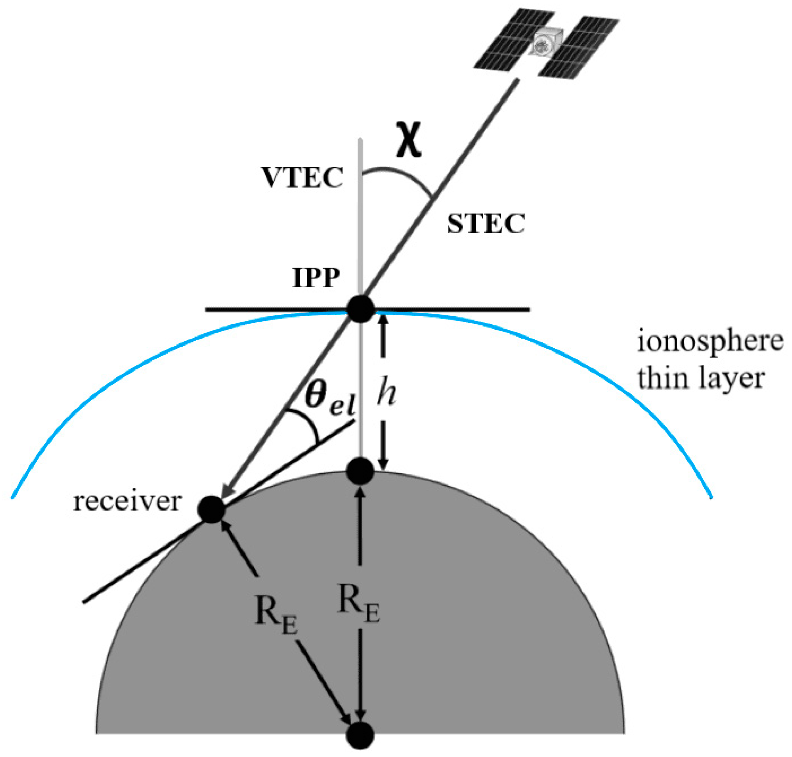
The H2PT model is an empirical thin-layer ionospheric model (TLIM), for which the main data source is 15-min Receiver INdependent EXchange Format (RINEX) files for the Regional Reference Frame Sub-Commission for Europe (EUREF) Permanent Network (EPN). Most TLIMs, such as the H2PT model, use an infinitely thin fixed-height layer [
18,
19]. The intersection of the pseudo line from the satellite (line of sight, LOS) to the receiver occurs at a given height, determining the ionospheric pierce point (IPP). This scheme is shown in
Figure 1 below.
Using this approximation, a two-dimensional ionospheric map can be created by converting the slant total electron content (STEC) to vertical total electron content (VTEC) using a formula from [
21]:
where
is the angle between the zenith direction and the satellite direction from the IPP.
The disadvantages of this method are the means of errors generated by model simplifications and the fixed IPP height. The global ionosphere TEC maps provided by the IGS Ionospheric Analysis Center use an IPP height of 450 km [
18,
22,
23]. Some researchers proposed the use of different heights in different ionospheric conditions or applications [
24,
25]. The new feature of the H2PT model is the possibility to generate new maps based on user-defined IPP heights (such a request would have to be submitted to the authors of the model).
The current version of the software allows us to use support procedures to perform calculation and generate maps of IPP heights with the following options:
Fixed height of the ionosphere—typically 350 or 450 km;
Hourly height estimated from the NeQuick-G electron density model as the balanced height for which the top and bottom densities are equal;
Hourly height of combined electron densities from the bottom electron density based on ionosonde measurement plus the scaled top profile from the NeQuick-G model; in case of less informative ionograms, the full NeQuick-G electron density profile can be used through the injections of ionospheric parameters;
Hourly hmF2 height plus correction factor, where the correction factor is defined as a constant by the researchers.
For this work, the calculation was performed with a fixed IPP height of 350 km for the Europe region.
The computational procedure of the H2PT model consists of the following steps:
Data acquisition:
- a.
RINEX observation files;
- b.
RINEX navigation files (Almanac data, Galileo ionospheric message);
- c.
Ionospheric parameters from recognized ionograms.
Computation of GNSS satellite position and data reviewing:
- a.
Generation of IPP height based on user options;
- b.
Calculating STEC [
21,
26,
27] (which does not take phase correction into account) for continuous observational arcs longer than 15 min—elimination of discontinuities;
- c.
Elimination of carrier phase shifts (whereby the ambiguity estimation is based on the Least-squares AMBiguity Decorrelation Adjustment (LAMBDA) method [
28]; data are also checked for outlier observations, and jumps are defined if the TEC value changes in subsequent observation epochs by more than 0.1 TECU; in this case, the arc is split at the jump point. If the length of the resulting arc is at least 15 min, it is still included in the calculation).
Calculation of observation geometry assuming the estimated IPP height (according to the diagram shown in
Figure 1).
Computation of VTEC separately for each available station (every 30 s) and evaluation of phase correction (as a sum of satellite and receiver phase biases) for each arc using the least-squares method (LSM). LSM fitting is performed for all arches within the 12-h period. The time window is shifted by 6 h and the operation is repeated.
Computation of VTEC values in all IPPs using Formula (1) according to
Figure 1.
Binning the obtained VTEC values according to the given grid (1° × 1° or 5° × 5°) and time resolution (for a given grid node, all IPPs with a margin of ± requested spatial resolution and ± time resolution are collected).
Computation of VTEC as a median value from the binned data.
The process runs automatically every 15 min with a 1-day delay, which is necessary to obtain all available RINEX files from the European region. It is also possible to build a near-real-time local model based on the stream data from permanent GNSS stations.
Discontinuities sometimes occur in the model, with no data for some nodes in some observation epochs. These discontinuities result from too few calculated VTEC values from a station in a given epoch to determine the median for a given node. The reason may be too few observation arcs for a given station, or delays in providing data by the station. It can be considered as a H2PT disadvantage, but the purpose of this procedure is to ensure a high quality of the resulting maps.
The model is still in development, and future features will allow it to perform additional analysis related to the area variation in TEC values, which can be compared with the local rate of TEC index (ROTI). It is planned to make the final version of the H2PT software available to the ionospheric community for public use.
3. Comparison Data
The ionospheric maps generated by the IGS cover the entire globe, and solutions in the final version are available at a delay of about 11 days. The files in the IONEX format contain data with a time resolution of 2 h, while their spatial resolution (latitude × longitude) is 2.5° × 5°. The data were downloaded from the National Aeronautics and Space Administration (NASA) Crustal Dynamics Data Information System (CDDIS) archive (
https://urs.earthdata.nasa.gov/, accessed on 20 October 2022), which contains datasets based on space and satellite geodesy techniques. The solution created by the Geodynamics Research Laboratory, University of Warmia and Mazury (GRL/UWM) [
29,
30] was chosen. In this study, IGS VTEC maps were used as reference VTEC measurements through which the performance of the H2PT model was evaluated.
All computations and visualizations were made in the MATLAB environment and involved data collection, processing, cataloguing, completeness control, performing calculations, determining statistics, and generating maps and plots.
4. Comparative Analysis between Models
The TEC values of the H2PT model and IGS maps in Europe for the period from January to March 2019 with an interval of 2 h were developed using the 5° × 5° grid version, then increased to 1° × 1°, while the IGS VTEC map data were interpolated as its nominal resolution is 2.5° × 5°. Differences between the models were determined and visualized, and their statistical parameters were calculated for the specific epochs under consideration. In the next stage, time series covering the period of a specific day were prepared, showing that the TEC parameter is variable according to latitude.
4.1. TEC Maps
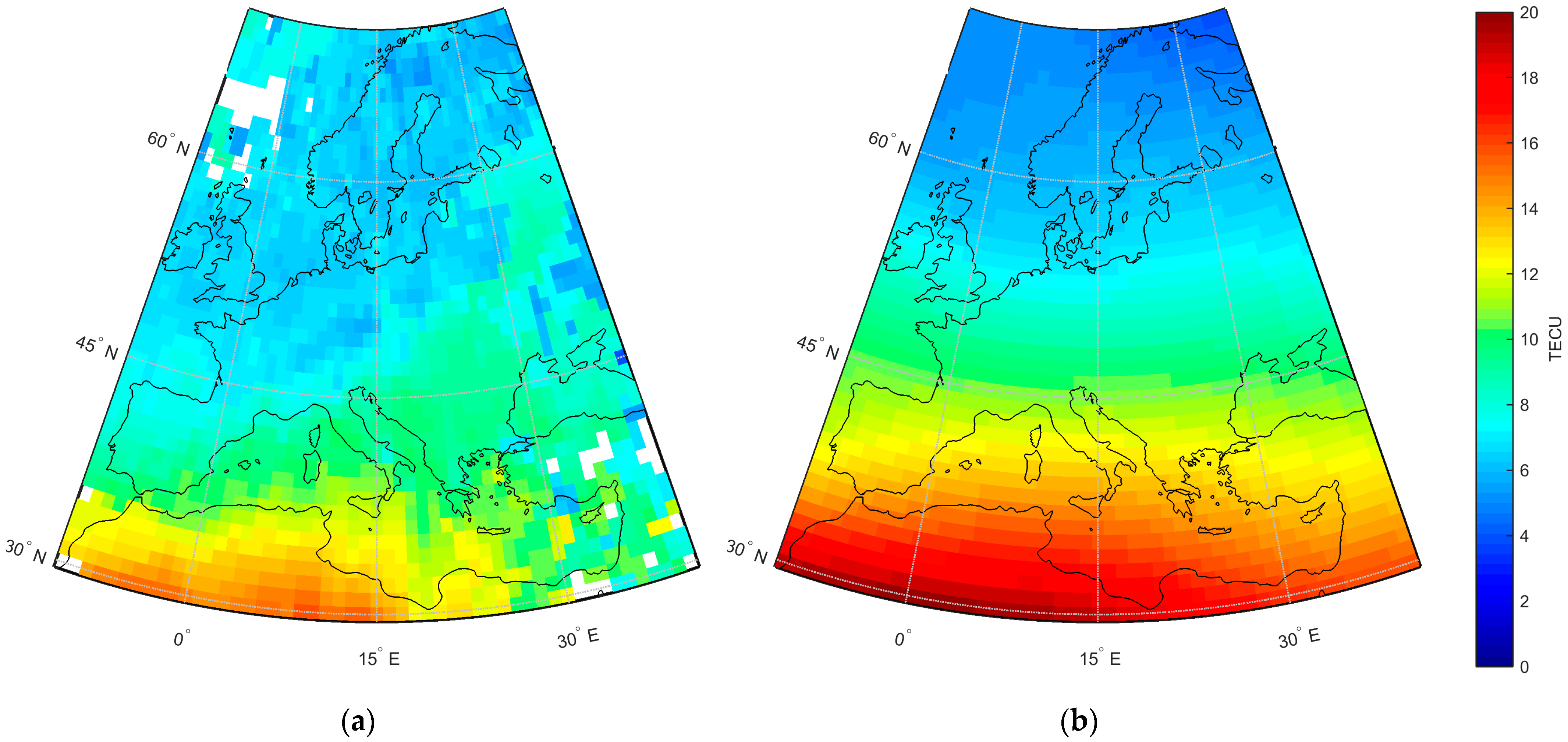
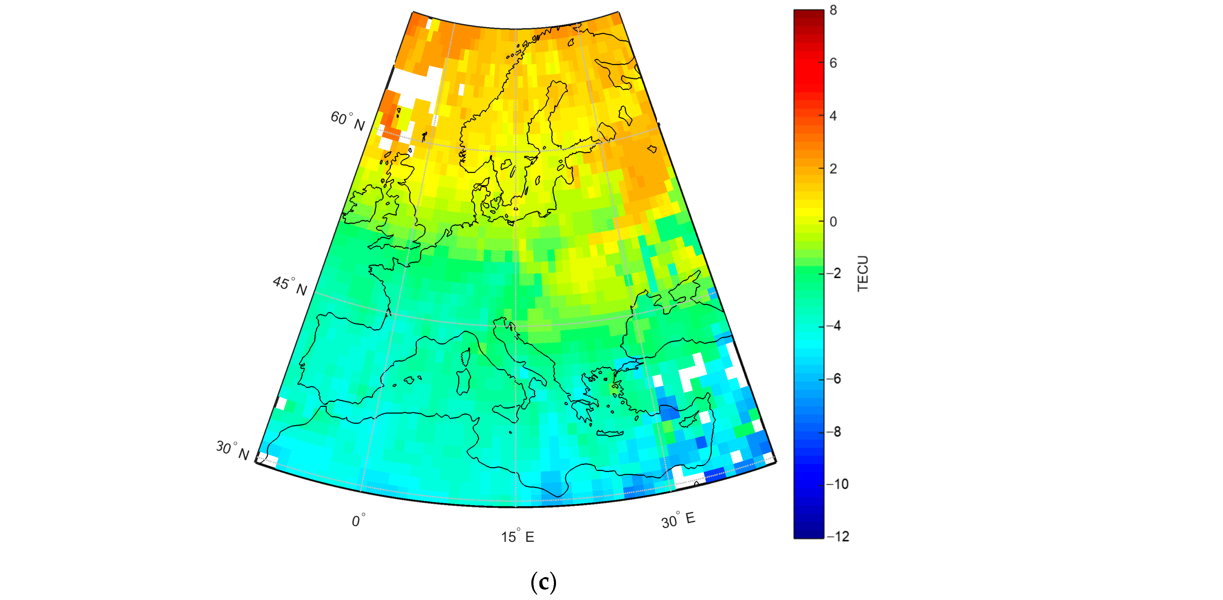
The data were visualized on the map of Europe, and a common, uniform scale was used for the H2PT model and IGS VTEC maps (from 0 to 20 TECU). A TEC map of the H2PT model, the IGS, and the differences between them was generated for each epoch.
Figure 2 and
Figure 3 show an example set for a relatively quiet day, 10 March 2019, at 14:00 UTC, at a resolution of 5° × 5° and 1° × 1°, respectively.
4.2. Statistical Parameters
As an addition to the plots, the statistical parameters of the models and the difference between them were computed for each of the considered epochs (
Table 1 and
Table 2, for a 5° and 1° grid, respectively). The differences
between the H2PT model values (
) and the IGS VTEC values (
for subsequent epochs
were determined as follows:
The tables include the basic parameters referring to the corresponding
(H2PT, IGS, or
), i.e., the minimum (3) and maximum (4) values and the maximum range
(5) in a given dataset (containing
elements), as well as further indicators, the formulas for which are presented below based on [
31,
32]. These include the mean
(6), standard deviation
(7), root-mean-square error (RMSE) (8), normalized root-mean-square error (NRMSE) (9), and Pearson correlation coefficient
(10):
Furthermore, analogous indices were determined for individual latitudes (
Table 3 and
Table 4, for the 5° and 1° grid, respectively). Consistent with the results presented in
Figure 2 and
Figure 3, the information contained in the tables are related to 10 March 2019, at 14:00 UTC.
4.3. Time Series
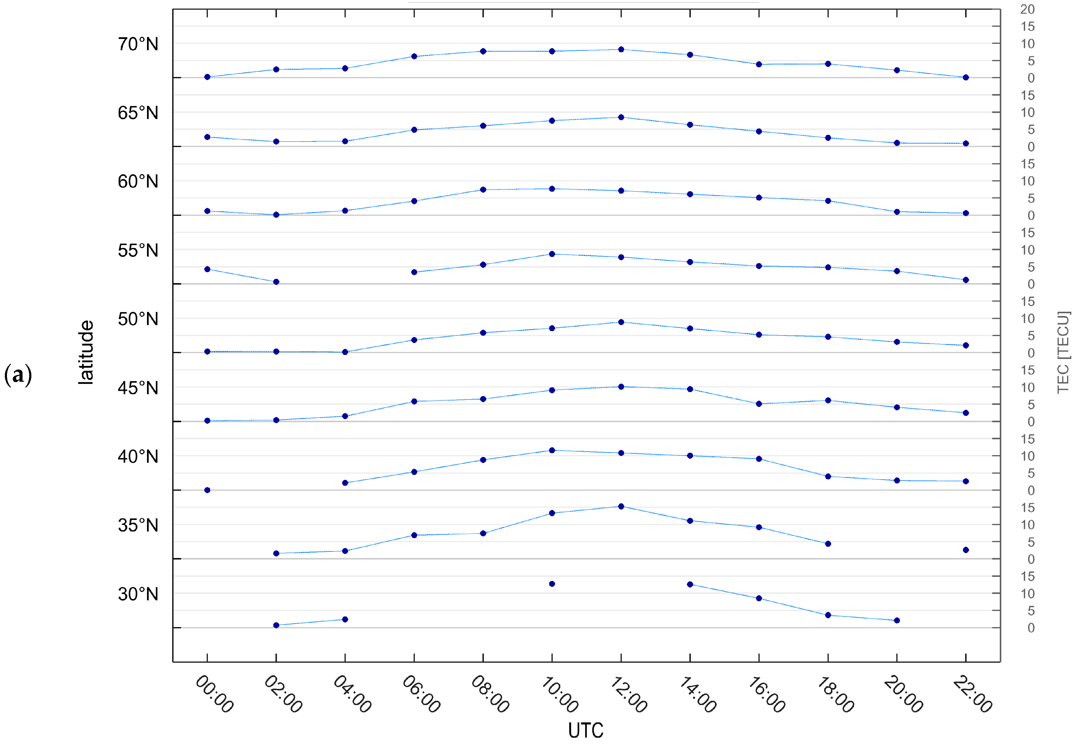
In the next stage, time series were generated, showing variation in the TEC parameter along individual meridians depending on the latitude and time of day.
Figure 4 shows the data for the 20°E meridian for 10 March 2019.
4.4. Discussion
In this section, available data for the period from January to March 2019 were examined and visualized, with a time interval of two hours (imposed by the resolution of the IGS VTEC map) at resolutions of 5° × 5° and 1° × 1°. The graphs and tables presented for 10 March 2019 are in line with the general trend that we noticed when compiling the H2PT model and IGS maps for other dates. The comparison indicates the occurrence of differences in the values of the TEC parameter, which are particularly depending on the latitude. At high latitudes, the values of the H2PT model are higher than those of the IGS VTEC maps (overestimated), whereas they are lower in tropical regions (underestimated). As the differences between the models generally amount to several TECUs, this may be related to the accuracy of the model itself. When considering the correlation of the models along a given parallel, no constant relationship is observed, whereas when considering the time of day, a larger correlation coefficient is observed in daytime. The RMSE values at successive parallels indicate that much smaller errors occur at high latitudes. However, when moving closer to the equator, where the activity of the ionosphere is increasing and more variable over the course of a day, the RMSE increases more.
The availability of the H2PT model data depends on the time of day (there are more missing nodes at nighttime), and there is also less availability in its edge fragments.
A comparison of the usefulness of the two different spatial resolutions of 5° × 5° and 1° × 1° reveals that, while the 5° × 5° grid allows general analyses showing trends of ionosphere behavior in Europe, the 1° × 1° grid gives the opportunity to carry out detailed interpretations, especially in the context of ionospheric disturbances.
5. Analysis of H2PT Model Solutions
In the next stage, the H2PT model data were developed using the 1° × 1° grid with an interval of 15 min, which is undoubtedly an advantage of this version compared to the commonly used IGS solution. Similar to the previous analysis phase, the data were visualized on the map of Europe, and basic statistical parameters were determined for each of the datasets. Daily time series were then generated for the 21°E meridian (approximate longitude of Warsaw) and the parallel Warsaw station nearby (52°N), taking into account a 3° buffer to the south and the north. The datasets present data for a day during which both positive and negative ionospheric disturbances were recorded, as well as for a quiet day or the daily median determined for the month in question.
5.1. TEC Maps
For each epoch, a map of the TEC parameter was generated, which was recorded in the .png format as well as the .gif format, producing 96 maps per day and creating a visualization in the form of a movie. The sample data are presented in
Figure 5, again for 10 March 2019, at 00:00, 4:00, 8:00, 12:00, 16:00, and 20:00 UTC.
5.2. Statistical Parameters
Similar to the comparison of the H2PT model and IGS VTEC maps discussed above, a statistical summary was generated showing the higher time resolution for the H2PT model at the selected epochs on 10 March 2019 (
Table 5).
5.3. Time Series
Using the collections posted on the RWC Warsaw website, disturbance catalogues for the Warsaw location (52°N, 21°E) were downloaded, as well as a set of data on positive/negative days and quiet days in Europe. The catalog was used to select the potential days when there would be a chance to observe disturbances on the maps. However, these dates are indicated in relation to the median for the whole month; therefore, a similar tactic was used in our analyses, and potentially disturbed days (positively and negatively) were also compared with the median calculated in two ways. Using a number of possible combinations, time series were generated to produce visualizations for disturbed and calm days (examples are shown in
Figure 6,
Figure 7 and
Figure 8) or the daily median (examples are shown in
Figure 9,
Figure 10 and
Figure 11). The median was determined in two ways (for each node independently): as a common value for the entire month, and separately for each of the 15-min epochs.
5.3.1. Positively Disturbed, Negatively Disturbed, and Quiet Days
The first discussed set contains the time series for positively and negatively disturbed days, in reference to a quiet day.
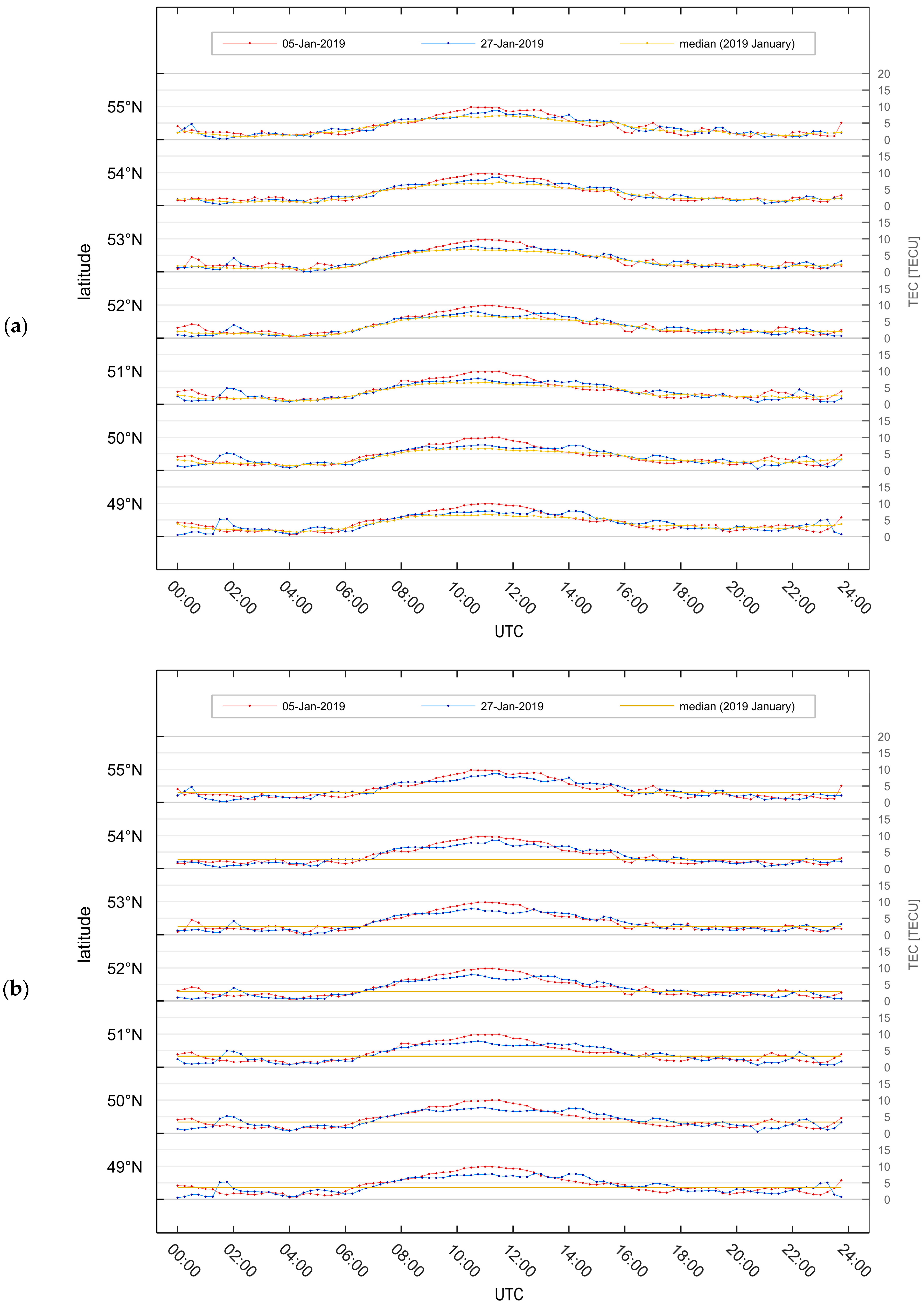
Although the catalogue of disturbances dedicated to Warsaw lacks information on the course of disturbances, 5 January 2019 was among the days characterized by an increase in ionospheric activity in Europe.
Figure 6 shows a clear increase in the TEC parameter from 8:00 to 13:00 UTC. In contrast, on 17 January 2019, a negative disturbance, according to the disturbance catalogue, occurred at 20:00 UTC; therefore, a decrease in TECU units can be seen. The disturbance did not appear at the same time on all the parallels shown, but moved from south to north over time, and simultaneously decreased and returned to normal values.
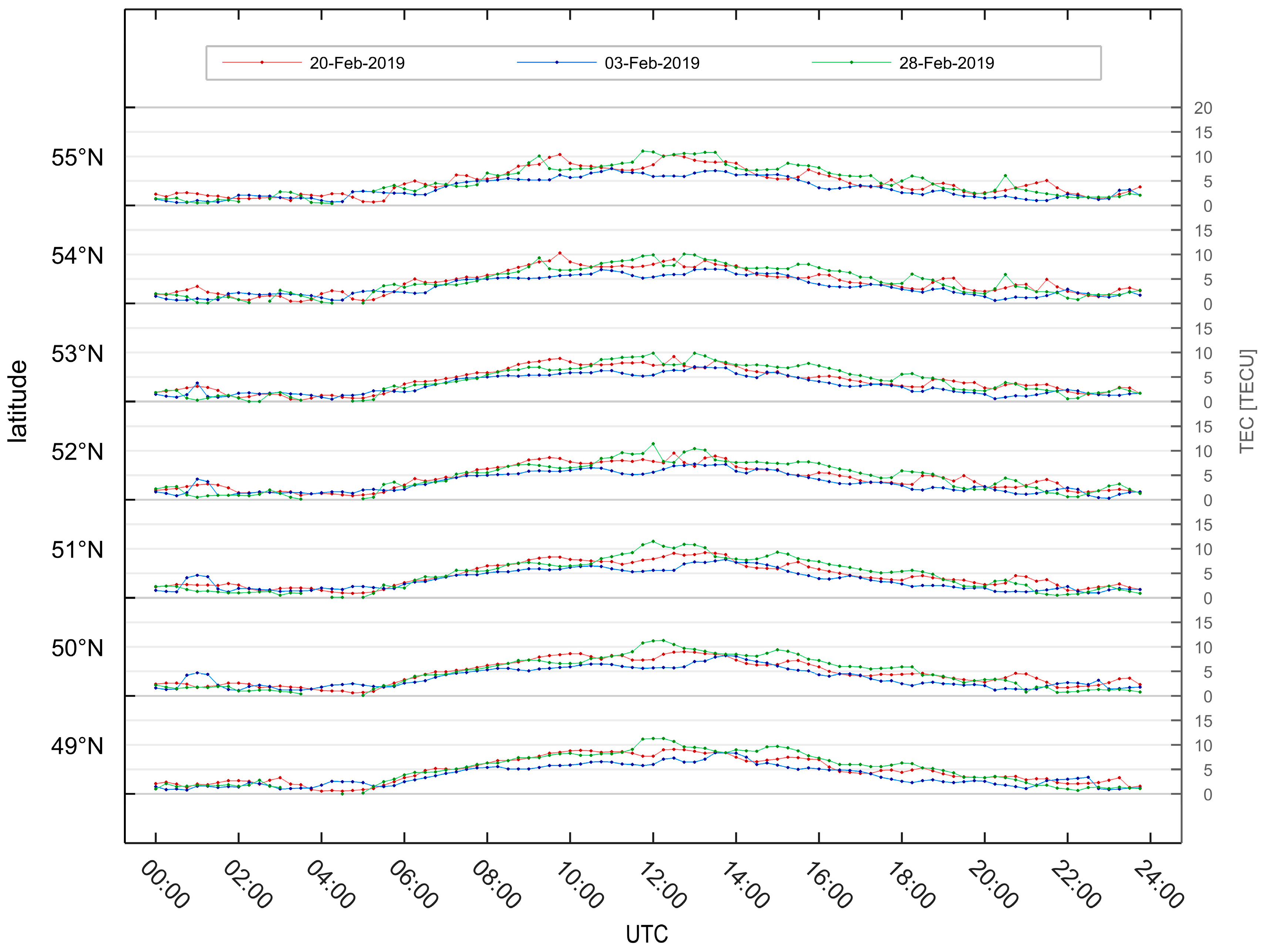
The last day of February was placed in the ranking as the calmest of the month, but the largest disturbances that occurred (119% and 138% from 16:00 to 19:00 and at 21:00 UTC, respectively) are not reflected in the TEC. Moreover, the variability in the parameter on the quiet day indicates the occurrence of disturbances, in particular at around 12:00 and 15:00 UTC. For 3 February 2019,
Figure 7 shows an underestimation in TEC values from 7:00 to 13:00 UTC, and further underestimation from 17:00 to 22:00 UTC, although the catalogue data indicate that disturbances occurred from 3:00 to 10:00 and from 18:00 to 00:00 UTC.
On 17 March 2019 (nominally negatively disturbed), it is difficult to observe any clear deviations from the series (
Figure 8), illustrating the course of the TEC on a quiet day during a disturbance (from 22:00 UTC); however, a clear decrease in the parameter can be seen a little earlier, from 15:00 to 21:00 UTC. During the positively disturbed day (28 March 2019), the TEC is similar to that expected for a quiet day, so no apparent increase can be seen from 18:00 to 20:00 UTC, as indicated by the information in the catalogue.
5.3.2. Positively Disturbed, Negatively Disturbed, and Median
In this section, sets containing two figures are presented. In each case, the first set shows positively and negatively disturbed days, with the median calculated for subsequent 15-min epochs, and the second set shows the positively and negatively disturbed days with the median for the whole day.
For January (
Figure 9), the TEC values for a calm day and the median are very similar. On 5 January 2019, there is a clear increase in TEC around noon, while on 17 January there is a slight decrease in the parameter relative to the median. Considering the next month (
Figure 10), it should be noted that the TEC size of a quiet day (28 February 2019,
Figure 7) differs considerably from the median. Correspondingly, the positive disturbance on 22 February 2019 is clear, as is the negative disturbance on 3 February 2019. For March, there is a significant deviation between the TEC of a non-disturbed day (31 March 2019,
Figure 7) and the median (
Figure 11), especially in the afternoon. Comparing this with 28 March 2019, when a positive disturbance was recorded, its occurrence can be confirmed from 15:00 to 21:00 UTC (although the catalogue includes the period from 18:00 to 20:00 UTC).
5.4. Discussion
The H2PT model data were processed at 15-min intervals and a resolution of 1° × 1° for the entire period in question. The generated maps provide the basis for analyzing individual disturbances in the state of the ionosphere, while the set of statistical parameters allows the recording of general trends to characterize the variability in the activity of the ionized atmosphere layer during a daily course.
Similar to the examples of the time series presented, the TEC values during many disturbances (both positive and negative), as well as numerous combinations between them (within a given month), were analyzed. The information contained in the catalogue of disturbed days is not always reflected in the joint combination with the median or the time series of a quiet day.
Considering the two approaches presented, as a result of the discrepancy between the illustrative catalogues for Europe and for the Warsaw station, the median is a more objective and neutral reference than a time series for a quiet day. Considering the method of quiet-day determination, unifying it for the whole month, regardless of the time of day, introduces far too much simplification; reducing data with a repetitive, variable course to a single value results in the loss of some information. Therefore, subsequent analyses should choose the option of determining the median for each epoch during the day separately.
6. Conclusions
The H2PT model is of a regional nature and is dedicated to Europe, which allows it to focus on a relatively small area with high resolution. Its undoubted advantage is resolution; maps are generated for epochs of every 15 min, while its grid (in a more accurate version) has dimensions of 1° × 1° (latitude × longitude). As the IGS VTEC maps have an interval of two hours and a spatial resolution of 2.5° × 5°, it is necessary to interpolate the data. Artificial smoothing can lead to many irregularities and eliminate ongoing ionospheric disturbances. The duration of such disturbances is usually just a few hours, and they cannot be expected to be clearly reflected on maps or time series presenting data with a 2-h interval.
The exemplary results presented in this study, as illustrated by the H2PT and IGS VTEC map sets, show the diversity of model characteristics. The 5° × 5° H2PT model significantly blurs locally occurring disturbances; thus, the 1° × 1° version is definitely more useful for detailed analysis of changes in the state of the ionosphere. In the case of the IGS VTEC maps with a lower spatial resolution, adaptation to a 1° × 1° grid via the interpolation of data obviously causes a forced result. However, the most visible differences between the two solutions are the differences related to latitude: there are higher TEC values from the H2PT model than the IGS VTEC maps in the north of the study area and lower in the southern fragment, with these differences being greater at night than during the day.
The analysis of the H2PT model data with a higher time resolution (15 min) and a 1° × 1° grid allows the detection of disturbances that last only a few hours and, therefore, cannot be reliably displayed using 2-h data. The course of the TEC parameter for the days during which a positive or negative disturbance occurred gives a reliable view compared with the median calculated independently for each epoch during the day. The median for the entire month introduces too much data degradation because it eliminates the typical variability in ionospheric activity during a daily course. A detailed examination of the disturbances listed in the catalogues indicates the occurrence of deviations between the presumably occurring disturbances and the median. Correspondingly, some of the positive or negative disturbances turn out to be not different from the median, and in other cases, the TEC values of positive disturbances are smaller than the mentioned parameter and, analogously, they are larger during negative disturbances. In addition, in many cases, the duration of the disturbance differs from the result of the comparison with the reference (median), and uncatalogued positive and negative deviations are observed.
In summary, these analyses have made it possible to become familiar with the characteristics of the H2PT ionosphere model, as well as to study its advantages and disadvantages. The relatively high temporal and spatial resolution is undoubtedly an advantage of the H2PT model because, unlike global models, this regional model allows conscientious analysis of ionospheric characteristics for the region of Europe. These analyses also indicated in which circumstances the H2PT model best reflects the behavior of the ionosphere and allowed us to find the model’s shortcomings in some conditions. Unfortunately, the incompleteness of the maps, especially at night and in higher spatial resolution, is a significant limitation of the model, indicating a direction for its improvement. On the other hand, a key advantage of the H2PT model lies in its numerical transparency and operability. This entails that within a single cell of either 5° × 5° or 1° × 1°, raw VTEC data from the receivers are present. The final value in a specific node is computed as the median of the existing measurement data only. This approach does mean that occasionally, due to insufficient data, the value for a certain node may not be determined. Nevertheless, it is important to consider that other models attempt to forcefully supplement data, and such an approach might result in erroneous conclusions when assessing the ionosphere’s state based on GNSS measurements. The developed model serves as an analytical tool for consolidating data sourced from GNSS measurements, which will also allow analysis if the correctness of other ionospheric models, such as NeQuick-G, IRI, Klobuchar, or other IGS solutions, based on real measurement datasets. The other considered issue is improving the efficiency of calculation; additionally, it is planned to generate maps of ROTI scintillations.
However, relatively dense surface coverage enables detailed analyses of passing disturbances in the ionosphere, while a small interval allows the detection of short-term changes. Certainly, it is necessary to expand the analysis of the H2PT model, which is why there are plans to extend the relevant period to include all seasons and the changing ionospheric activity during the course of the 25th solar cycle. The H2PT model can also potentially be used as a new solution for determining the ionospheric correction in the course of GNSS observation data processing for the European region. In this context, an important point for further research on the H2PT model will be its analysis compared to the navigation models: NeQuick-G and Klobuchar.
Author Contributions
Conceptualization, P.G., A.Ś., Ł.T. and M.P.; methodology, P.G. and A.Ś.; software, P.G., Ł.T. and M.P.; validation, P.G., Ł.T. and M.P.; formal analysis, P.G., A.Ś., Ł.T. and M.P.; investigation, P.G. and A.Ś.; resources, Ł.T., M.P. and P.G.; data curation, Ł.T., M.P. and P.G.; writing—original draft preparation, P.G. and Ł.T.; writing—review and editing, P.G., A.Ś., Ł.T. and M.P.; visualization, P.G.; supervision, A.Ś.; project administration, A.Ś.; funding acquisition, A.Ś. All authors have read and agreed to the published version of the manuscript.
Funding
This research was funded by the Polish Ministry of Education and Science from funds for science in 2020 allocated to the implementation of a co-financed international project.
Data Availability Statement
Conflicts of Interest
The authors declare no conflict of interest.
References
- Teunissen, P.J.G.; Montenbruck, O. Springer Handbook of Global Navigation Satellite Systems; Springer International Publishing AG: Cham, Switzerland, 2017; ISBN 9783319429267. [Google Scholar]
- Savchuk, S.; Hiryak, I. Evaluation of Static GNSS Positioning Accuracy during Selected Normal and High Ionospheric Activity Periods. Tech. Sci./Univ. Warm. Maz. Olsztyn 2015, 18, 299–311. [Google Scholar]
- Seeber, G. Satellite Geodesy; Walter de Gruyter: Berlin, Germany, 2003; Volume 2, ISBN 3110175495. [Google Scholar]
- Mainul, M.; Jakowski, N. Ionospheric Propagation Effects on GNSS Signals and New Correction Approaches. In Global Navigation Satellite Systems: Signal, Theory and Applications; IntechOpen: Rijeka, Croatia, 2012. [Google Scholar] [CrossRef]
- Narkiewicz, J. GPS i Inne Satelitarne Systemy Nawigacyjne; Wydawnictwa Komnikacji i Łączności: Warszawa, Poland, 2007; ISBN 978-83-206-1642-2. [Google Scholar]
- Krypiak-Gregorczyk, A.; Wielgosz, P.; Borkowski, A. Ionosphere Model for European Region Based on Multi-GNSS Data and TPS Interpolation. Remote Sens. 2017, 9, 1221. [Google Scholar] [CrossRef]
- Wielgosz, P.; Krypiak-Gregorczyk, A.; Borkowski, A. Regional Ionosphere Modeling Based on Multi-GNSS Data and TPS Interpolation. In Proceedings of the 2017 Baltic Geodetic Congress (BGC Geomatics), Gdansk, Poland, 22–25 June 2017; pp. 287–291. [Google Scholar] [CrossRef]
- Czarnecki, K. Geodezja Współczesna; Wydawnictwo Naukowe PWN SA: Warszawa, Poland, 2014; ISBN 978-83-01-18011-9. [Google Scholar]
- Specht, C. System GPS; Wydawnictwo Bernardinum Sp. z o. o.: Pelplin, Poland, 2007; ISBN 978-83-7380-469-2. [Google Scholar]
- Davies, K.; Hartmann, G.K. Studying the Ionosphere with the Global Positioning System. Radio Sci. 1997, 32, 1695–1703. [Google Scholar] [CrossRef]
- Hofmann-Wellenhof, B.; Lichtenegger, H.; Wasle, E. GNSS—Global Navigation Satellite Systems—GPS, GLONASS, Galileo, and More; SpringerWienNewYork: Wien, Austria, 2007; ISBN 9783211730126. [Google Scholar]
- Hernández-Pajares, M.; Wielgosz, P.; Paziewski, J.; Krypiak-Gregorczyk, A.; Krukowska, M.; Stepniak, K.; Kaplon, J.; Hadas, T.; Sosnica, K.; Bosy, J.; et al. Direct MSTID Mitigation in Precise GPS Processing. Radio Sci. 2017, 52, 321–337. [Google Scholar] [CrossRef]
- Bilitza, D.; Altadill, D.; Truhlik, V.; Shubin, V.; Galkin, I.; Reinisch, B.; Huang, X. International Reference Ionosphere 2016: From Ionospheric Climate to Real-Time Weather Predictions. Space Weather 2017, 15, 418–429. [Google Scholar] [CrossRef]
- European Union. European GNSS (Galileo) Open Service—Ionospheric Correction Algorithm for Galileo Single Frequency Users. 2016. Available online: https://www.gsc-europa.eu/sites/default/files/sites/all/files/Galileo_Ionospheric_Model.pdf (accessed on 23 May 2023).
- Nava, B.; Coïsson, P.; Radicella, S.M. A New Version of the NeQuick Ionosphere Electron Density Model. J. Atmos. Sol.-Terr. Phys. 2008, 70, 1856–1862. [Google Scholar] [CrossRef]
- Okoh, D.; Seemala, G.; Rabiu, B.; Habarulema, J.B.; Jin, S.; Shiokawa, K.; Otsuka, Y.; Aggarwal, M.; Uwamahoro, J.; Mungufeni, P.; et al. A Neural Network-Based Ionospheric Model Over Africa From Constellation Observing System for Meteorology, Ionosphere, and Climate and Ground Global Positioning System Observations. J. Geophys. Res. Space Phys. 2019, 124, 10512–10532. [Google Scholar] [CrossRef]
- Klos, Z.; Stanislawska, I.; Dziak-Jankowska, B. Heliogeophysical Prediction Service in Poland:Past, Present and Future. Hist. Geo Space Sci. 2019, 10, 193–199. [Google Scholar] [CrossRef]
- Mannucci, A.J.; Wilson, B.D.; Yuan, D.N.; Ho, C.H.; Lindqwister, U.J.; Runge, T.F. A Global Mapping Technique for GPS-Derived Ionospheric Total Electron Content Measurements. Radio Sci. 1998, 33, 565–582. [Google Scholar] [CrossRef]
- Brunini, C.; Camilion, E.; Azpilicueta, F. Simulation Study of the Influence of the Ionospheric Layer Height in the Thin Layer Ionospheric Model. J. Geod. 2011, 85, 637–645. [Google Scholar] [CrossRef]
- Hein, W.Z.; Kashiva, Y.; Goto, Y.; Kasahara, Y. Estimation Method of Ionospheric TEC Distribution from Single Frequency GPS Measurements Using a Slant Effect Model. In Proceedings of the 2016 URSI Asia-Pacific Radio Science Conference (URSI AP-RASC), Seoul, Republic of Korea, 21–25 August 2016; IEEE: Seoul, Republic of Korea, 2016; pp. 104–106. [Google Scholar]
- Hernández-Pajares, M.; Juan, J.M.; Sanz, J.; Aragón-Àngel, À.; García-Rigo, A.; Salazar, D.; Escudero, M. The Ionosphere: Effects, GPS Modeling and the Benefits for Space Geodetic Techniques. J. Geod. 2011, 85, 887–907. [Google Scholar] [CrossRef]
- Hernández-Pajares, M.; Juan, J.M.; Sanz, J.; Orús, R. Second-Order Ionospheric Term in GPS: Implementation and Impact on Geodetic Estimates. J. Geophys. Res. Solid Earth 2007, 112, 1–16. [Google Scholar] [CrossRef]
- Jiang, H.; Jin, S.; Hernández-Pajares, M.; Xi, H.; An, J.; Wang, Z.; Xu, X.; Yan, H. A New Method to Determine the Optimal Thin Layer Ionospheric Height and Its Application in the Polar Regions. Remote Sens. 2021, 13, 2458. [Google Scholar] [CrossRef]
- Klobuchar, J. Ionospheric Time-Delay Algorithm for Single-Frequency GPS Users. IEEE Trans. Aerosp. Electron. Syst. 1987, AES-23, 325–331. [Google Scholar] [CrossRef]
- Li, Z.; Yuan, Y.; Wang, N.; Hernandez-Pajares, M.; Huo, X. SHPTS: Towards a New Method for Generating Precise Global Ionospheric TEC Map Based on Spherical Harmonic and Generalized Trigonometric Series Functions. J. Geod. 2015, 89, 331–345. [Google Scholar] [CrossRef]
- Wielgosz, P.; Milanowska, B.; Krypiak-Gregorczyk, A.; Jarmołowski, W. Validation of GNSS-Derived Global Ionosphere Maps for Different Solar Activity Levels: Case Studies for Years 2014 and 2018. GPS Solut. 2021, 25, 103. [Google Scholar] [CrossRef]
- Zhang, Y.; Wu, F.; Kubo, N.; Yasuda, A. TEC Measurement By Single Dual-Frequency GPS Receiver. In Proceedings of the 2003 International Symposium on GPS/GNSS, Tokyo, Japan, 15–18 November 2003. [Google Scholar]
- Teunissen, P.J.G. The Least-Squares Ambiguity Decorrelation Adjustment: A Method for Fast GPS Integer Ambiguity Estimation. J. Geod. 1995, 70, 65–82. [Google Scholar] [CrossRef]
- Hernández-Pajares, M.; Juan, J.M.; Sanz, J.; Orus, R.; Garcia-Rigo, A.; Feltens, J.; Komjathy, A.; Schaer, S.C.; Krankowski, A. The IGS VTEC Maps: A Reliable Source of Ionospheric Information since 1998. J. Geod. 2009, 83, 263–275. [Google Scholar] [CrossRef]
- Hernández-Pajares, M.; Roma-Dollase, D.; Krankowski, A.; García-Rigo, A.; Orús-Pérez, R. Methodology and Consistency of Slant and Vertical Assessments for Ionospheric Electron Content Models. J. Geod. 2017, 91, 1405–1414. [Google Scholar] [CrossRef]
- Janssen, P.H.M.; Heuberger, P.S.C. Calibration of Process-Oriented Models. Ecol. Modell. 1995, 83, 55–66. [Google Scholar] [CrossRef]
- Cohen, J. Statistical Power Analysis for the Behavioral Sciences, 2nd ed.; New York University: New York, NY, USA, 1988; ISBN 0-8058-0283-5. [Google Scholar]
Figure 1.
Conversion model from slant total electron content (STEC) to vertical total electron content (VTEC) in a thin-layer ionospheric model (TLIM) [
20].
Figure 1.
Conversion model from slant total electron content (STEC) to vertical total electron content (VTEC) in a thin-layer ionospheric model (TLIM) [
20].
Figure 2.
Total electron content (TEC) maps for 10 March 2019, at 14:00 UTC, at a spatial resolution of 5° × 5°: (a) H2PT model; (b) IGS VTEC map; and (c) difference between them.
Figure 2.
Total electron content (TEC) maps for 10 March 2019, at 14:00 UTC, at a spatial resolution of 5° × 5°: (a) H2PT model; (b) IGS VTEC map; and (c) difference between them.
Figure 3.
TEC maps for 10 March 2019, at 14:00 UTC, at a spatial resolution of 1° × 1°: (a) H2PT model; (b) IGS VTEC map; and (c) difference between them.
Figure 3.
TEC maps for 10 March 2019, at 14:00 UTC, at a spatial resolution of 1° × 1°: (a) H2PT model; (b) IGS VTEC map; and (c) difference between them.
Figure 4.
Time series for the 20°E meridian for 10 March 2019: (a) H2PT model; (b) IGS VTEC map; and (c) differences between them.
Figure 4.
Time series for the 20°E meridian for 10 March 2019: (a) H2PT model; (b) IGS VTEC map; and (c) differences between them.
Figure 5.
TEC maps for the H2PT model for 10 March 2019, at (a) 00:00; (b) 4:00; (c) 8:00; (d) 12:00; (e) 16:00; and (f) 20:00 UTC.
Figure 5.
TEC maps for the H2PT model for 10 March 2019, at (a) 00:00; (b) 4:00; (c) 8:00; (d) 12:00; (e) 16:00; and (f) 20:00 UTC.
Figure 6.
TEC time series at a longitude of 21°E for a positively disturbed day (5 January 2019), a negatively disturbed day (17 January 2019), and a quiet day (6 January 2019).
Figure 6.
TEC time series at a longitude of 21°E for a positively disturbed day (5 January 2019), a negatively disturbed day (17 January 2019), and a quiet day (6 January 2019).
Figure 7.
TEC time series at a longitude of 21°E on a positively disturbed day (22 February 2019), a negatively disturbed day (3 February 2019), and a quiet day (28 February 2019).
Figure 7.
TEC time series at a longitude of 21°E on a positively disturbed day (22 February 2019), a negatively disturbed day (3 February 2019), and a quiet day (28 February 2019).
Figure 8.
Time series at a longitude of 21°E for a positively disturbed day (28 March 2019), a negatively disturbed day (17 March 2019), and a quiet day (31 March 2019).
Figure 8.
Time series at a longitude of 21°E for a positively disturbed day (28 March 2019), a negatively disturbed day (17 March 2019), and a quiet day (31 March 2019).
Figure 9.
Time series at a longitude of 21°E for a positively disturbed day (5 January 2019) and a negatively disturbed day (17 January 2019), along with the median of (a) particular epochs and of (b) the whole day.
Figure 9.
Time series at a longitude of 21°E for a positively disturbed day (5 January 2019) and a negatively disturbed day (17 January 2019), along with the median of (a) particular epochs and of (b) the whole day.
Figure 10.
Time series at a longitude of 21°E for a positively disturbed day (22 February 2019) and a negatively disturbed day (3 February 2019), along with the median of (a) particular epochs and of (b) the whole day.
Figure 10.
Time series at a longitude of 21°E for a positively disturbed day (22 February 2019) and a negatively disturbed day (3 February 2019), along with the median of (a) particular epochs and of (b) the whole day.
Figure 11.
Time series at a longitude of 21°E for a positively disturbed day (28 March 2019) and negatively disturbed day (17 March 2019), along with the median of (a) particular epochs and of (b) the whole day.
Figure 11.
Time series at a longitude of 21°E for a positively disturbed day (28 March 2019) and negatively disturbed day (17 March 2019), along with the median of (a) particular epochs and of (b) the whole day.
Table 1.
Statistical parameters of the H2PT model, the IGS VTEC map, and their differences at a spatial resolution of 5° × 5° (date: 10 March 2019, at 14:00 UTC).
Table 1.
Statistical parameters of the H2PT model, the IGS VTEC map, and their differences at a spatial resolution of 5° × 5° (date: 10 March 2019, at 14:00 UTC).
| Name | Min
(TECU) | Max
(TECU) | Range
(TECU) | Mean
(TECU) | Standard Deviation
(TECU) | RMSE
(TECU) | NRMSE
(-) | Correlation Coefficient
(-) |
|---|
| H2PT | 6.3 | 13.5 | 7.2 | 8.28 | 2.09 | 2.93 | 0.35 | 0.96 |
| IGS | 3.9 | 19.8 | 15.9 | 9.71 | 4.50 |
| −6.4 | 2.4 | 8.8 | −1.43 | 2.57 | | | |
Table 2.
Statistical parameters of the H2PT model, the IGS VTEC map, and their differences at a spatial resolution of 1° × 1° (date: 10 March 2019, at 14:00 UTC).
Table 2.
Statistical parameters of the H2PT model, the IGS VTEC map, and their differences at a spatial resolution of 1° × 1° (date: 10 March 2019, at 14:00 UTC).
| Name | Min
(TECU) | Max
(TECU) | Range
(TECU) | Mean
(TECU) | Standard Deviation
(TECU) | RMSE
(TECU) | NRMSE
(-) | Correlation Coefficient
(-) |
|---|
| H2PT | 4.0 | 15.8 | 11.8 | 8.23 | 2.22 | 2.65 | 0.32 | 0.90 |
| IGS | 3.9 | 19.8 | 15.9 | 9.55 | 4.07 |
| −8.5 | 3.3 | 11.8 | −1.35 | 2.28 | | | |
Table 3.
Statistical parameters of the differences between the H2PT model and the IGS VTEC map for individual latitudes at a spatial resolution of 5° × 5° (date: 10 March 2019, at 14:00 UTC).
Table 3.
Statistical parameters of the differences between the H2PT model and the IGS VTEC map for individual latitudes at a spatial resolution of 5° × 5° (date: 10 March 2019, at 14:00 UTC).
φ
(°) | Min
(TECU) | Max
(TECU) | Range
(TECU) | Mean
(TECU) | Standard Deviation
(TECU) | RMSE
(TECU) | NRMSE
(-) | Correlation Coefficient
(-) |
|---|
| 70 | 1.5 | 2.4 | 0.9 | 2.01 | 0.29 | 2.03 | 0.25 | 0.79 |
| 65 | 1.0 | 2.2 | 1.2 | 1.29 | 0.38 | 1.34 | 0.16 | 0.12 |
| 60 | 0.3 | 1.5 | 1.2 | 0.75 | 0.34 | 0.82 | 0.10 | −0.21 |
| 55 | −0.5 | 1.2 | 1.7 | −0.13 | 0.53 | 0.53 | 0.06 | −0.27 |
| 50 | −2.2 | −0.2 | 2.0 | −1.27 | 0.80 | 1.48 | 0.18 | −0.29 |
| 45 | −3.2 | −1.5 | 1.7 | −2.39 | 0.70 | 2.48 | 0.30 | −0.02 |
| 40 | −3.4 | −2.8 | 0.6 | −3.15 | 0.24 | 3.15 | 0.38 | 0.94 |
| 35 | −4.5 | −3.3 | 1.2 | −4.09 | 0.36 | 4.11 | 0.50 | 0.94 |
| 30 | −6.4 | −5.1 | 1.3 | −5.92 | 0.44 | 5.93 | 0.72 | 0.97 |
Table 4.
Statistical parameters of the differences between the H2PT model and the IGS VTEC map for individual latitudes at a spatial resolution of 1° × 1° (date: 10 March 2019, at 14:00 UTC).
Table 4.
Statistical parameters of the differences between the H2PT model and the IGS VTEC map for individual latitudes at a spatial resolution of 1° × 1° (date: 10 March 2019, at 14:00 UTC).
φ
(°) | Min
(TECU) | Max
(TECU) | Range
(TECU) | Mean
(TECU) | Standard Deviation
(TECU) | RMSE
(TECU) | NRMSE
(-) | Correlation Coefficient
(-) |
|---|
| … | | | | | | | | |
| 43 | −4.1 | −1.6 | 2.5 | −2.62 | 0.71 | 2.71 | 0.33 | 0.53 |
| 42 | −4.0 | −1.8 | 2.3 | −2.89 | 0.63 | 2.96 | 0.36 | 0.64 |
| 41 | −5.8 | −1.9 | 3.9 | −3.30 | 0.90 | 3.42 | 0.42 | 0.57 |
| 40 | −5.1 | −2.1 | 3.0 | −3.28 | 0.60 | 3.34 | 0.41 | 0.75 |
| 39 | −5.1 | −1.4 | 3.7 | −3.48 | 0.66 | 3.54 | 0.43 | 0.81 |
| 38 | −6.0 | −2.0 | 4.0 | −3.56 | 0.71 | 3.62 | 0.44 | 0.81 |
| 37 | −7.0 | −2.3 | 4.7 | −3.73 | 0.88 | 3.83 | 0.47 | 0.73 |
| 36 | −7.6 | −2.4 | 5.1 | −3.96 | 0.96 | 4.07 | 0.49 | 0.77 |
| 35 | −6.3 | −1.4 | 4.9 | −3.76 | 0.81 | 3.84 | 0.47 | 0.77 |
| … | | | | | | | | |
Table 5.
Statistical parameters of the H2PT model for selected epochs (date: 10 March 2019).
Table 5.
Statistical parameters of the H2PT model for selected epochs (date: 10 March 2019).
| UTC | Min
(TECU) | Max
(TECU) | Range
(TECU) | Mean
(TECU) | σ
(TECU) |
|---|
| 00:00 | 0.0 | 6.2 | 6.2 | 1.33 | 1.03 |
| 4:00 | 0.0 | 5.1 | 5.1 | 1.77 | 0.88 |
| 8:00 | 1.7 | 12.6 | 10.9 | 6.58 | 1.73 |
| 12:00 | 5.8 | 18.2 | 12.4 | 9.54 | 1.66 |
| 16:00 | 2.5 | 12.7 | 10.2 | 6.34 | 1.93 |
| 20:00 | 0.0 | 7.9 | 7.9 | 2.53 | 1.30 |
| Disclaimer/Publisher’s Note: The statements, opinions and data contained in all publications are solely those of the individual author(s) and contributor(s) and not of MDPI and/or the editor(s). MDPI and/or the editor(s) disclaim responsibility for any injury to people or property resulting from any ideas, methods, instructions or products referred to in the content. |
© 2023 by the authors. Licensee MDPI, Basel, Switzerland. This article is an open access article distributed under the terms and conditions of the Creative Commons Attribution (CC BY) license (https://creativecommons.org/licenses/by/4.0/).


