Sea Ice Detection from GNSS-R Data Based on Residual Network

Abstract

Sea ice is an important component of the polar circle and influences atmospheric change. Global navigation satellite system reflectometry (GNSS-R) not only realizes time-continuous and wide-area sea ice detection, but also greatly reduces the cost of sea ice remote sensing research, which has been a hot topic in recent years. To tackle the challenges of noise interference and the reduced accuracy of sea ice detection during the melting period, this paper proposes a sea ice detection method based on a residual neural network (ResNet). ResNet addresses the issue of vanishing gradients in deep neural networks and introduces residual connections, which allows the network to reuse learned features from previous layers. Delay-Doppler maps (DDMs) collected from TechDemoSat-1 (TDS-1) are used as input, and National Oceanic and Atmospheric Administration (NOAA) surface-type data above 60°N are selected as the true values. Based on ResNet, the sea ice detection achieved an accuracy of 98.61%, demonstrating high robustness to noise and strong stability during the sea ice melting period (June to September). In comparison to other sea ice detection algorithms, it stands out with its advantages of high accuracy, stability, and insensitivity to noise.

1. Introduction

In recent years, the Arctic sea ice has shown a rapid decline due to global warming [1], which has attracted continuous attention worldwide. Currently, there are mainly two methods for sea ice detection: visible light remote sensing and microwave remote sensing [2,3]. However, visible light remote sensing is vulnerable to natural phenomena such as clouds and fog, which makes continuous observation impossible. Microwave remote sensing requires high-cost investment. The emergence of GNSS-R [4] technology provides a more efficient and economical way to obtain sea ice data.

GNSS-R is a highly promising remote sensing technology that has wide-ranging applications in areas including wind speed estimation [5,6,7,8], soil moisture monitoring [9,10,11,12], water body detection [13], lake ice remote sensing [14] and estimation of sea surface roughness [15]. The delay-Doppler map (DDM) acquired by TDS-1 has facilitated sea ice remote sensing studies. In 2016, Yan [16] conducted research based on TDS-1 data and proposed a new way for sea ice detection using DDM observation such as pixel number (PN), power summation (PS), geometric center (GC) distance, center-of-mass (CM) distance, and CM taxicab distance as DDM observation metrics. In 2017, Zhu [17] calculated the difference between two adjacent DDMs and derived the corresponding number of pixels, which was used to distinguish between DDM images of seawater and sea ice by setting a threshold. Alonso-Arroyo [18] evaluated the coherence of DDMs and waveforms and verified the presence of sea ice using DDM average power (DDMA), trailing edge slope (TES), and matched filter (MF) as DDM observations. The rise in machine learning has provided new approaches for GNSS-R sea ice detection. In 2017, Yan [19] applied neural network theory to sea ice detection by training a network using DDMs from a training set and corresponding seawater/ice labels, and then inputting the processed DDM into the trained neural network to generate sea ice detection results. In 2018, Yan [20] first applied a convolutional neural network (CNN) to sea ice detection, which requires less data preprocessing than neural networks and can achieve higher accuracy in sea ice detection. In 2019, Yan [21] proposed a feature selection method for sea ice detection using the support vector machine (SVM) algorithm.

In communication systems, noise is an undesired signal caused by various disturbances and distortions. Higher values of SNR indicate a greater difference between the signal and the noise. By contrast, the lower the value of SNR the greater the effect of noise on the signal and the poorer the signal quality. Hu [22] classifies DDMs according to SNR and noise, and as the SNR deteriorates, the influence of noise becomes more and more serious, and the sea ice detection accuracy then shows a substantial decrease. Since most DDMs are subject to noise interference, GNSS-R sea ice detection uses DDMs with high SNR values, which significantly reduces DDM utilization. The annual sea ice melt period is from June to September. During this period sea ice sometimes appears as floating ice, and the physical form of this sea ice is in a constant process of change from ice to water. The floating ice has both sea ice and seawater characteristics on the DDM and is difficult to classify accurately, which is the reason for the reduced accuracy of sea ice detection. Problems such as the serious influence of noise on DDM data, low data utilization, and the sudden drop in sea ice detection accuracy during the melting period have not been adequately addressed in existing studies.

To address these problems, in this paper, DDMs are used as an input to ResNet [23], and NOAA surface-type data are used as the true values to train ResNet for sea ice detection. The residual module in ResNet enables the network to break through the limitation of network depth, and can effectively learn and capture complex features, which improves the robustness to noise and makes it insensitive to noise in DDMs. This gives ResNet better adaptability in sea ice detection, which improves the reliability of the results. In addition, during the melting period, the morphology and physical properties of the sea ice will change greatly, which affects the sea ice detection, and the ResNet model can better adapt to these input changes through its deep structure and residual connections, thus showing higher stability and accuracy in the sea ice detection during the melting period.

Section 2 introduces the theory of GNSS-R sea ice detection, including a detailed explanation of the delay-Doppler map (DDM), the structure of CNNs, and the sea ice detection process. In Section 3, the results are thoroughly discussed. Section 4 provides a summary of this paper.

2. Materials and Methods

2.1. Data Description

2.1.1. GNSS-R DDM Data

Launched in 2014 with a sampling rate of 16.367 MHz, TDS-1 carries the on-board GNSS remote sensing receiver SGR-ReSI with an orbital altitude of 635 km and an inclination of 98.4° and has eight payloads that rotate periodically to acquire different remote sensing data. The satellite provides L1B class data in NetCDF format. TDS-1 divides the day’s data into four groups of H00, H06, H12 and H18, and provides data such as DDM data and Metadata. In this paper, DDM data collected by TDS-1 from February to November 2015 are selected and divided into a training set and a validation set in a ratio of 7:3. DDM data from February to December 2018 are selected as the test set for the model test. Using one year of DDMs as the training set can allow the convolutional neural network to fully learn the features and tolerate the noise of DDMs, which is more conducive to improving detection accuracy. The angle of incidence at which GNSS signals propagate towards the Earth’s surface exerts an influence on signal attenuation, with greater angles of incidence resulting in increased path loss. Furthermore, for a consistent level of ocean surface roughness, higher incidence angles correspond to an amplified coherent scattering component, potentially leading to misidentifications of seawater as sea ice during sea ice detection. In this experimental dataset, all incidence angles employed are limited to values below 40 degrees. The areas we have chosen for study are all above 60°N latitude because of the large amount of sea ice present in these areas, which provides favorable conditions for the study of GNSS-R sea ice detection in the experiment. These locales exhibit pronounced seasonal fluctuations in sea ice. In winter, there is an expansion in sea ice coverage, leading to increased thickness. Conversely, during the summer season, rising temperatures facilitate sea ice melting, resulting in a reduction in sea ice cover and the emergence of open water.

GNSS-R is a remote sensing study based on GNSS signals reflected from the ground. The reflective surface of the ground is usually rough, so the ground-reflected signals received by the receiver from GNSS satellites are a series of multipath signals formed after reflecting over a large area around the reflection point. These multipath signals have different time delays and Doppler values due to differences in propagation paths and the motion of the receiver platform. A complete theoretical model for the scattering of GNSS signals was proposed in the literature [24] in 2000, which is a two-dimensional function of time delay and Doppler and can be used to obtain the reflected power at different scattering points. The expression is as follows:

$$Y(\tau ,f)=\frac{P_t{G}_t{\lambda }^2{T}_i^2}{{(4\pi )}^3}{\displaystyle {\iint }_A\frac{G_r{\Lambda }^2(\tau )S^2(f)}{R_t^2{R}_r^2}}{\sigma }^0\mathrm{d}A$$

(1)

where $Y(\tau ,f)$ is the signal correlation power processed by the receiver, a function of delay and Doppler, $P_t$ is the satellite transmit signal power, $G_t$ is the gain of the transmitter antenna, $G_r$ is the gain of the receiver antenna, $T_i$ is the coherent integration time in the signal, $R_t$ is the distance from the transmitter to the surface point, $R_r$ is the distance from the receiver to the surface point, ${\sigma }^0$ is the term related to the parameters of the reflecting surface, including the reflection coefficient and roughness, $\mathrm{S}(f)$ is the Doppler shift function, $\Lambda (\tau )$ is the GNSS code correlation function, and $A$ is the scattering effective area.

DDM data are produced by aggregating collected power distribution results and mapping the corresponding Doppler and time-delay coordinate positions. To create the DDM of sea surface scattering signals, the power distribution area in space is divided by equal time delay lines and equal Doppler frequency correlation lines. Points with the same time delay and Doppler frequency are then accumulated [19]. It is worth mentioning that an original TDS-1 DDM consists of 128 bins (with a resolution of 244 ns) in delay and 20 bins in Doppler (with a resolution of 500 Hz). Figure 1 shows the DDMs collected in seawater and sea ice, respectively.

DDMs consist of a certain number of equally sized grids, each of which is sized as the length of the delay interval multiplied by the length of the Doppler interval, with each grid corresponding to one signal power. Figure 1a is a seawater DDM, and Figure 1b is a sea ice DDM collected on the ice field. The difference between them indicates that the rough surface of seawater will reduce the overall coherent specular reflection, resulting in a larger scintillation area and more of the DDM being extended along the delay and Doppler axes. As shown in Figure 2a,b, a DDM is easily affected by noise, especially in the case of a seawater DDM. The noise impact caused by the rough surface of seawater is greater than on that of a sea ice DDM, so the classification accuracy of a seawater DDM is generally lower than that of a sea ice DDM, which is one of the reasons for the decrease in classification accuracy. By observing the DDM dataset, it was found that some sea ice was melting from June to September, and some of the melted sea ice DDMs are shown in Figure 2c. The classification characteristic of the DDMs is either sea ice or seawater, therefore, there are difficult-to-classify DDMs during sea ice melting periods, and the accuracy of the classification algorithm will decline from June to September.

2.1.2. Ground Truth Data

In this paper, the NOAA land surface type data are selected as the ground truth for sea ice detection. NOAA is a mapping product database of the National Oceanic and Atmospheric Administration in the United States. It provides a monthly summary database that can access monthly temperature, precipitation, and snowfall records worldwide, as well as surface type data including land, coastlines, rivers, lakes, sea ice, and seawater. NOAA uses a variety of advanced observation and measurement techniques to acquire data, including satellites, buoys, survey stations, aircraft, and ships, employing rigorous quality control and quality assurance procedures. This includes data calibration, correction, and ongoing monitoring and auditing. NOAA collaborates with international organizations and scientific institutions in other countries to share data and observations to ensure the consistency and accuracy of the global data. Data from NOAA are generally considered to be highly accurate and reliable. Each DDM has a corresponding latitude and longitude. The NOAA data are extracted from the DDM dataset according to the corresponding latitude and longitude to discriminate between land and sea, removing the DDM data from land, rivers, and lakes, and retaining only the DDM data from sea ice and seawater.

Sea ice is usually classified into two main types: first-year ice (FYI) and multi-year ice (MYI). These two types of ice have different characteristics and they also have different signal responses on GNSS-R signals. FYI sea ice forms during the cold winter months and is usually present for only one freezing season. This ice is usually thin because it has only one year to accumulate and grow. FYI is usually more susceptible to warm season melt than MYI because it is relatively less dense and more easily broken. MYI is sea ice that forms and accumulates throughout multiple freezing seasons and usually survives for many years. This ice is relatively thicker and denser because it has accumulated over many years. MYI is typically more stable and resistant to melting and fragmentation than FYI. FYI typically produces a weaker GNSS-R reflective signal because it is relatively thin and has an irregular surface, which is less capable of reflecting signals. MYI, on the other hand, typically produces a stronger GNSS-R reflected signal because it is relatively thick and has a flat surface, which makes it easier to reflect signals.

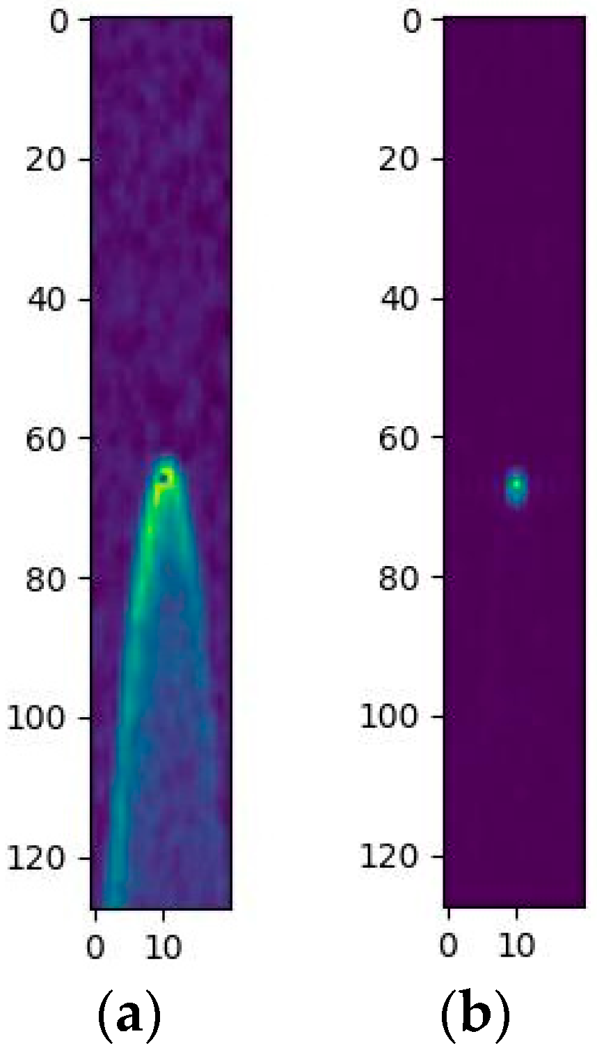
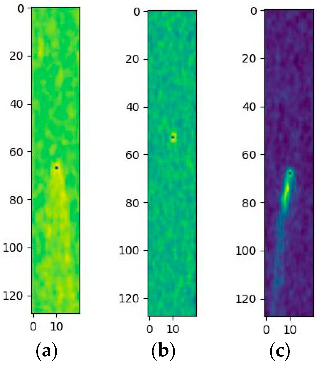
2.1.3. DDM Data Preprocessing

(1) Remove invalid data: according to the ground truth, remove DDM data from land, rivers, and lakes, and retain DDM data from sea ice and seawater.

(2) Remove baseline noise: to reduce the influence of system noise from the antenna and instrument in the DDM data, each element of DDM data needs to have baseline noise removed. Yan [25] has proposed many feasible methods for noise leveling. Al-Khaldi [26] proposes a method to exclude pixels in the non-coherent DDM as a way to reduce the effect of thermal noise. The pixel power must exceed a percentage of the maximum value of the DDM to be used in the calculation, i.e., pixels in the DDM that exceed 0.3 times the maximum value are used in the calculation. In this paper, the first four available delay rows (128) spanning all Doppler bins (20) in DDM data are selected as the area for calculating noise. The expression for calculating the noise value is as follows [19]:

$$\mathrm{Noise}=\frac{1}{X}{\displaystyle \sum _{\tau ={\tau }_1}^{{\tau }_2}{\displaystyle \sum _{f=f_1}^{f_2}\mathrm{DDM}}}(\tau ,f)$$

(2)

where $\mathrm{Noise}$ represents the noise value; ${\tau }_1$ and ${\tau }_2$ are the upper and lower bounds of delay in the noise calculation region, respectively; $f_1$ and $f_2$ are the upper and lower bounds of frequency delay in the noise calculation region, respectively; and $X$ is the number of pixels in the noise calculation region. After calculating the noise, in each DDM the noise is subtracted to reduce the noise interference. The expression is as follows:

$$DD{M}_{new}=Y(\tau ,f)-Noise$$

(3)

(3) Normalization: the DDM data need to be normalized after stripping the noise as the TDS-1 data have not been calibrated.

(4) Data stretching: the original size of the DDM is 128 × 20, which is not conducive to CNN extraction of features. Therefore, to ensure feature consistency and training efficiency of the convolutional neural network, the 128 × 20 DDM is reshaped into a 32*32 DDM by using bilinear interpolation.

Bilinear interpolation is a commonly used image processing to estimate the values of off-grid points when the values of the points are known. It is based on the idea of linear interpolation but performs linear interpolation in two dimensions at the same time, thus approximating the value of the target point more accurately. The calculation expression is as follows:

$$\begin{array}{l}f(x,y)\approx \frac{y_2-y}{y_2-y_1}f\left(R_1\right)+\frac{y-y_1}{y_2-y_1}f\left(R_2\right)\\ =\frac{y_2-y}{y_2-y_1}\left(\frac{x_2-x}{x_2-x_1}f\left(Q_{11}\right)+\frac{x-x_1}{x_2-x_1}f\left(Q_{21}\right)\right)+\frac{y-y_1}{y_2-y_1}\left(\frac{x_2-x}{x_2-x_1}f\left(Q_{12}\right)+\frac{x-x_1}{x_2-x_1}f\left(Q_{22}\right)\right)\end{array}$$

(4)

where the coordinates of $Q_{11}$ are $(x_1,y_1)$, of $Q_{12}$ are $(x_2,y_2)$, of $Q_{21}$ are $(x_2,y_1)$, of $Q_{22}$ are $(x_2,y_2)$, of $R_1$ are $(x,y_1)$, and of $R_2$ are $(x,y_2)$.

2.2. Convolutional Neural Network Algorithm

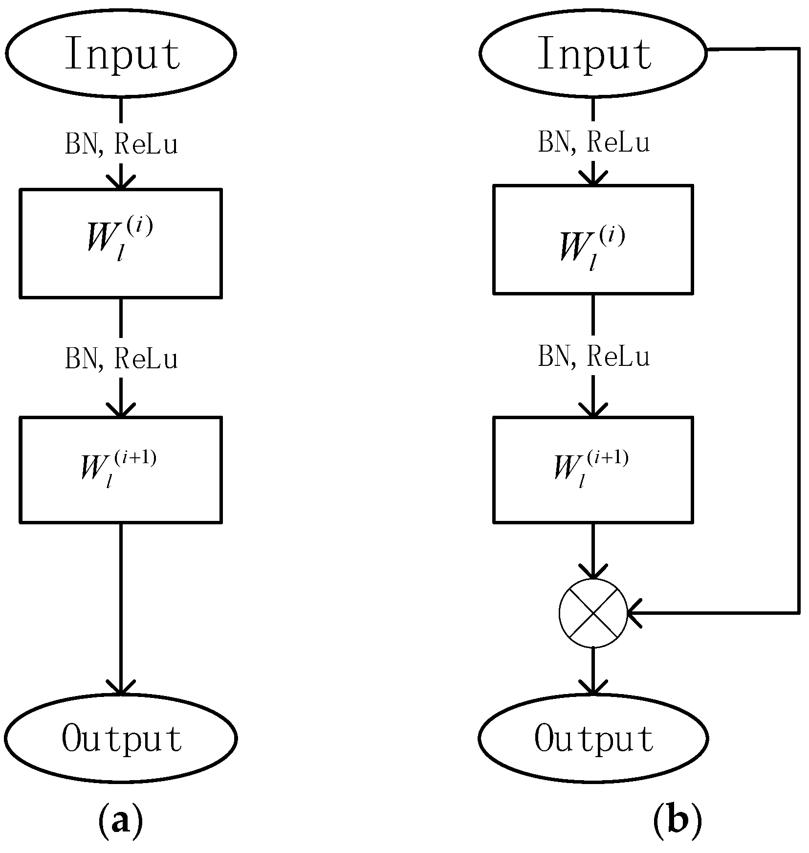
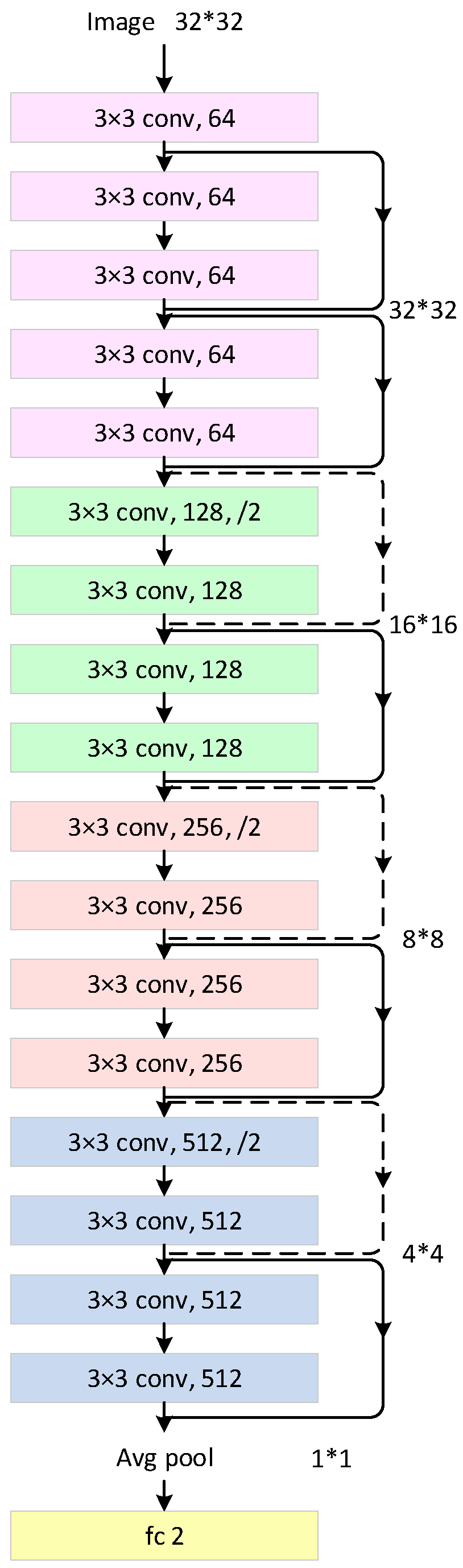
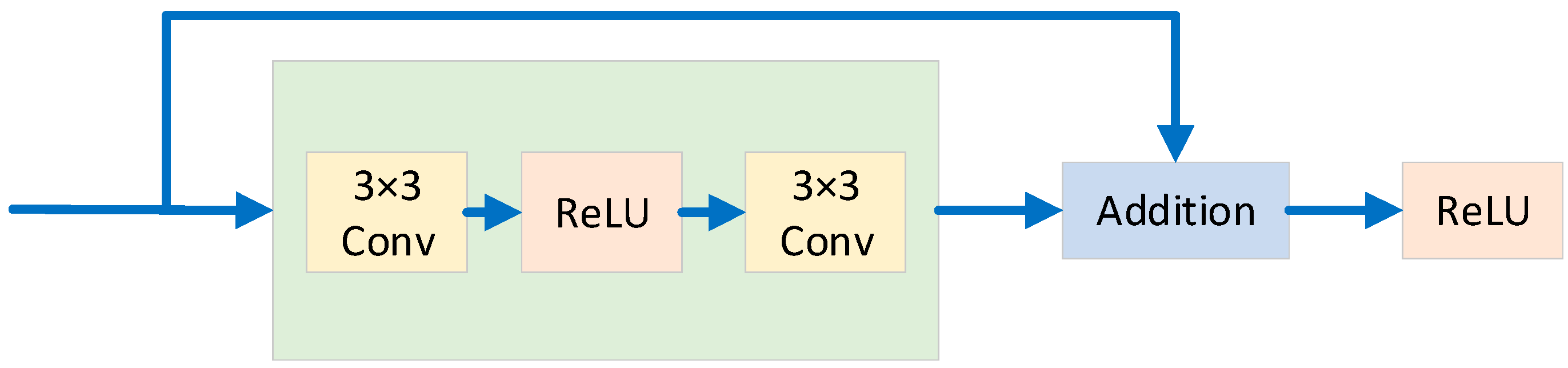
2.2.1. ResNet Algorithm

Convolutional neural networks are mainly composed of repeatedly superimposed convolutional kernels. As shown in Figure 3a, the underlying network mentioned here is the backbone of the convolutional neural network, where the input data are convolved to extract features. The input characteristics of the module are ${\mathrm{x}}_l$, $f$:$x_l$→$x_{l+1}$. The output of this layer can be described by:

$$x_{l+1}=f\left(x_l,\left\{W_l^{(i)}\right\}\right)=W_l^{(2)}\sigma \left(BN\left(W_l^{(1)}\sigma \left(BN\left(x_l\right)\right)\right)\right)$$

(5)

where $W_l^{(i)}$ and $\sigma$ are the $i$th ($i$ = 1, …, 5) weights and the activation function, respectively. The widely adopted rectified linear unit is chosen for $\sigma$, that is:

$$f(x)=\max (0,x)$$

(6)

The ResNet is a typical nonlinear single-step iterative equation. As shown in Figure 3b, the input characteristic of the module is ${\mathrm{x}}_l$. The output of this layer can be described by:

$$x_{l+1}=\sigma \left[f\left(x_l,\left\{W_l^{(i)}\right\}\right)\right]+x_l$$

(7)

As pointed out in [23], ResNet effectively addresses challenges such as network degradation, gradient dispersion, and gradient explosion. Consequently, ResNet architecture was employed in this study (refer to Figure 4), designed with inputs of dimensions 32 × 32 × 3. The ResNet model comprises a ResNet block, a Global AvgPooling layer, and an output layer.

Taking the initial ResNet block as an illustration (depicted in Figure 5), the residual block consists of two 3 × 3 convolutional layers, yielding an equivalent number of output channels. Subsequently, each convolutional layer is immediately followed by a batch normalization layer and a ReLU activation function. These convolutional layers are then connected by bypass connections, adding the input directly before the final ReLU activation function. The initial block maintains the same number of channels as the input channels. Each subsequent block doubles the number of channels compared to the previous block while halving the height and width.

The output layer is designed with two units and uses the softmax function as the activation function, which shows the probability of occurrence of sea ice or seawater:

$$\mathrm{Softmax}(\mathrm{x})=\frac{{\mathrm{e}}^{{\mathrm{x}}_{\mathrm{i}}}}{{\displaystyle \sum _{\mathrm{i}}{\mathrm{e}}^{{\mathrm{x}}_{\mathrm{i}}}}}$$

(8)

where $x_i$ is the input vector, $e^{x_i}$ is the exponential function of the natural constant e, and the Softmax function transforms each element in the input vector into a probability value, representing the probability of the input belonging to the $i$th category.

Because of the presence of blocks in ResNet, less is learned in the convolutional layer, and the full information is preserved with another constant equation of the block. The ResNet needs to learn less and be easy to train.

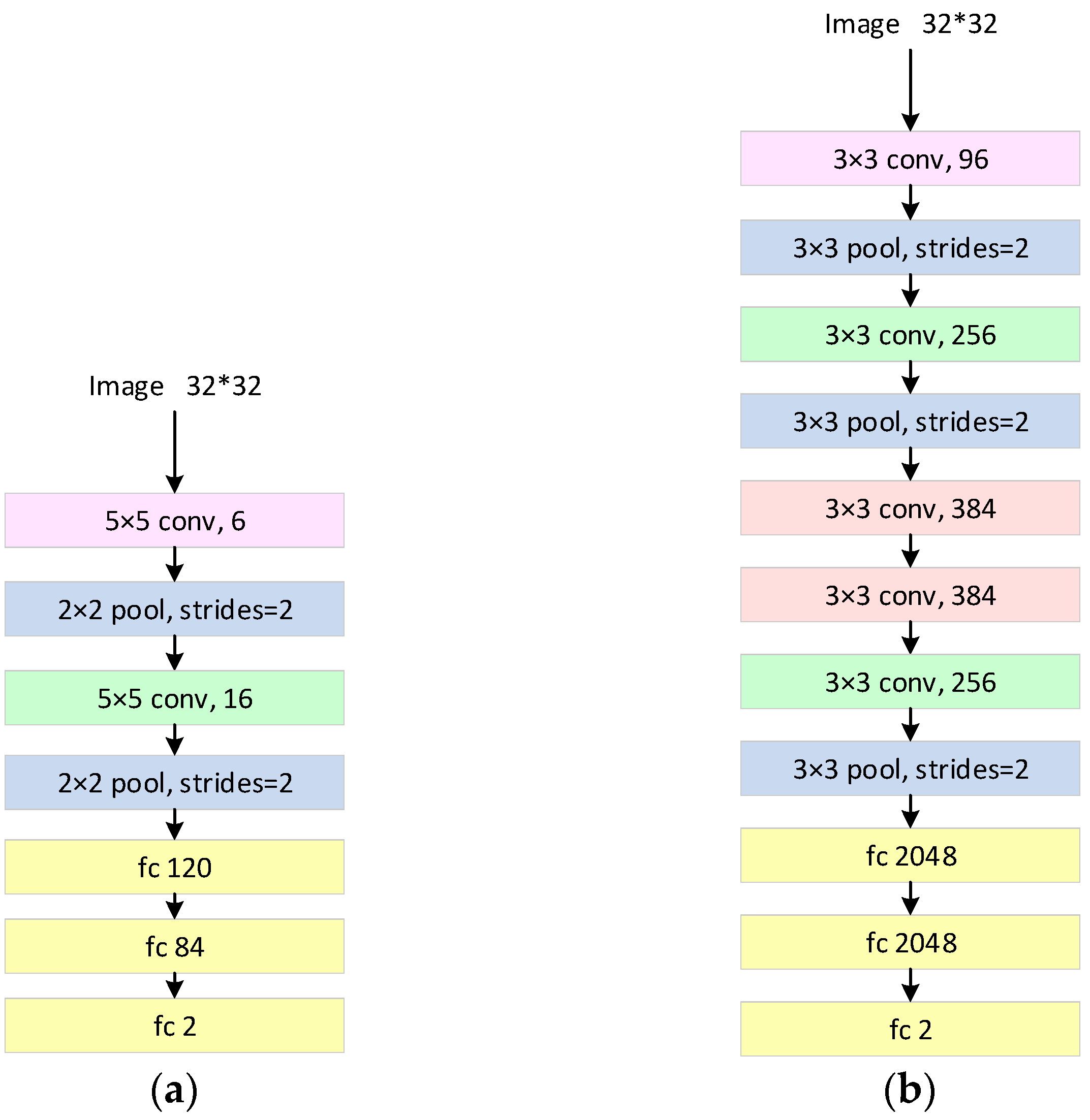
2.2.2. LeNet Algorithm

The LeNet network architecture comprises seven layers, as depicted in Figure 6a. These layers encompass two convolutional layers, three fully connected layers, and two pooling layers. The initial layer is a convolutional layer housing six convolutional kernels. Each of these kernels possesses dimensions of 5 × 5, employs a step size of 1, and incorporates zero padding. These convolutional kernels are responsible for extracting low-level features from the input image, such as edges and corner points, through the process of learning. Immediately following each convolutional layer is a pooling layer that executes a maximum pooling operation using a 2 × 2 window and a step size of 2, thereby reducing the size of the feature map. The second convolutional layer and its accompanying pooling layer in LeNet-5 are analogous to the preceding ones, with the exception that the second convolutional layer comprises 16 convolutional kernels. This layer stacking facilitates the capture of more abstract features. After the convolutional and pooling operations, LeNet-5 connects to two fully connected layers. The first fully connected layer consists of 120 neurons, while the second fully connected layer consists of 84 neurons. The third fully connected layer consists of 2 neurons, corresponding to the desired output classes.

2.2.3. AlexNet Algorithm

The structure of the AlexNet network is shown in Figure 6b. It contains 5 layers of convolutional layers, 3 layers of pooling layers, and 3 layers of fully connected layers. The network starts with a 32 × 32 input image, goes through convolution, pooling, and fully connected operations layer by layer, and finally outputs a prediction of the image category. The first convolutional layer consists of 96 convolutional kernels, each of size 3 × 3. After the first convolutional layer, followed by a maximum pooling layer, the pooling operation is performed using a 3 × 3 window with a step size of 2. The second convolutional layer consists of 256 convolutional layers of size 3 × 3, followed by a pooling layer. The third, fourth and fifth convolutional layers’ convolutional kernel size is still 3 × 3 and contains 384, 384, and 256 convolutional kernels respectively. Immediately after these convolutional layers are pooling layers. After the convolutional and pooling layers, AlexNet connects three fully connected layers. Both the first and second fully connected layers contain 2048 neurons, and the last fully connected layer outputs the score for the corresponding category.

2.3. Training of the CNN

The adaptive moment estimation (Adam) algorithm [27] was adopted for training. Adam combines the advantages of adaptive gradient algorithms (the AdaGrad method, which improves the performance of sparse gradient problems by preserving a learning rate for each parameter) and root mean square propagation (RMSProp, which adaptively preserves the learning rate for each parameter based on the mean of the nearest magnitude of the weighted gradient). Adam is an extension of the gradient descent optimization algorithm, which is very effective when dealing with large amounts of data or a large number of parameters involved.

The cross-entropy function was chosen as the loss function, which is generally used in conjunction with the Softmax activation function. The formula of the loss function is as follows:

$$\mathrm{Loss}=-{\displaystyle \sum _{i=1}^{\begin{array}{c}\mathrm{output}\\ \mathrm{size}\end{array}}{y}_i}\cdot \log {\widehat{y}}_i$$

(9)

where $y_i$ is the true value of the label, and ${\widehat{y}}_i$ is the predicted value of the model. The true labels of each sample were compared with their corresponding predicted results, and their probability values were then logarithmically calculated. Next, by multiplying it with the one-hot encoding of the true label, only the probability values corresponding to the true label were retained. Finally, the results of all samples were summed up and averaged to obtain the final loss value.

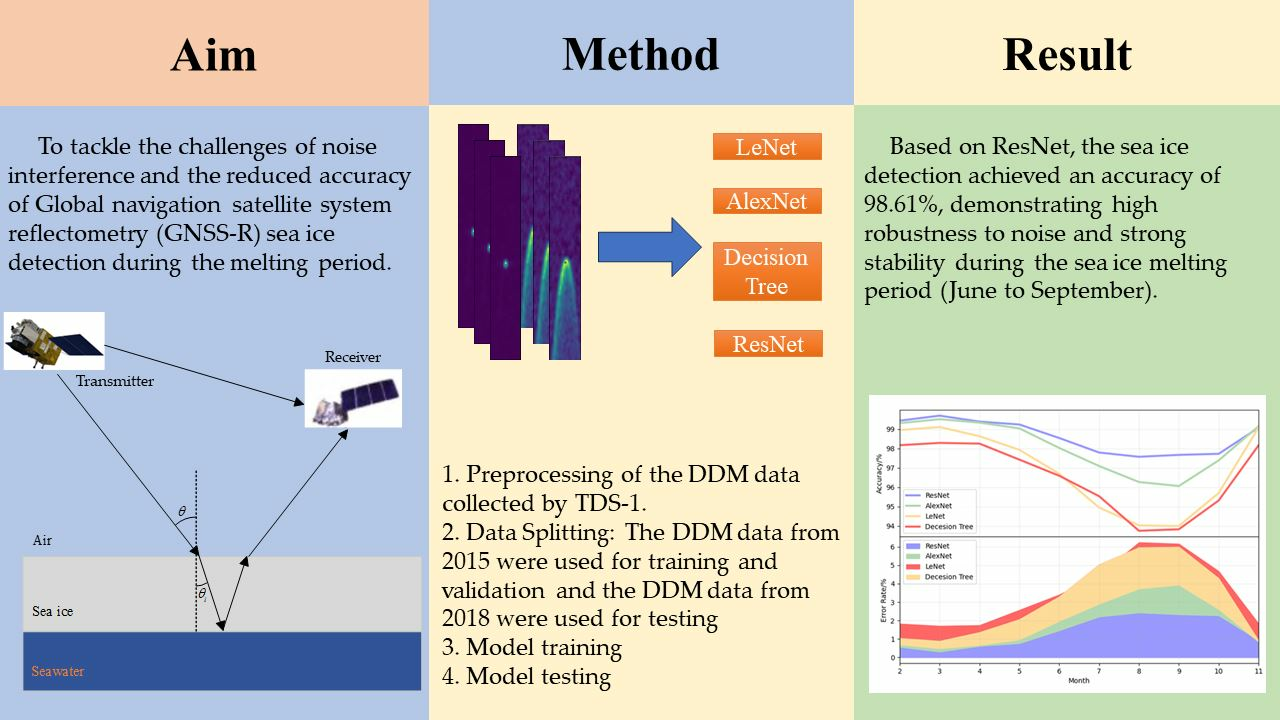
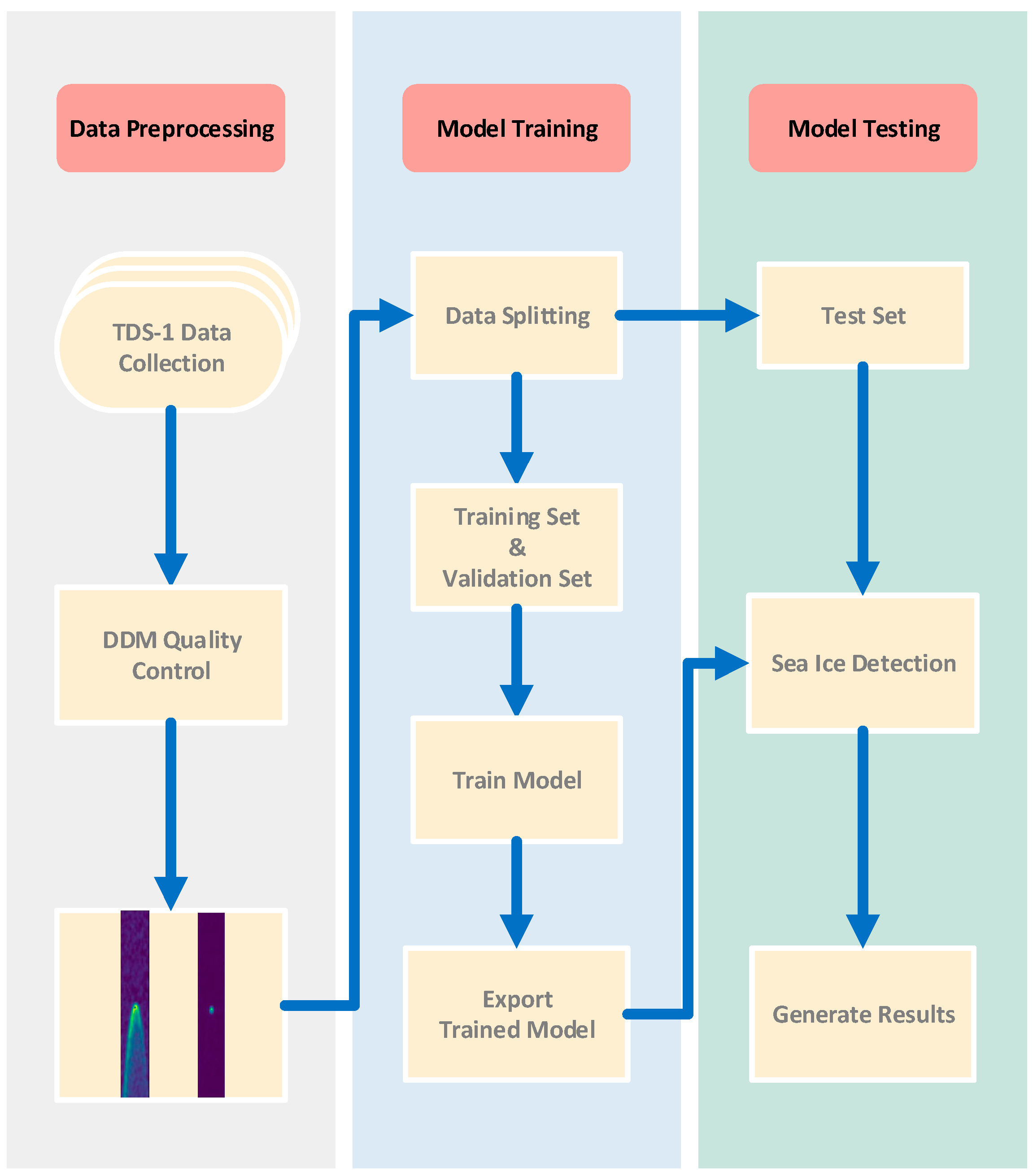
2.4. Process of GNSS-R Sea Ice Detection

The sea ice detection algorithm process includes three steps: data processing, model training, and model testing. The flowchart of the sea ice detection algorithm is shown in Figure 7, and the specific steps are as follows:

• Preprocessing of the DDM data collected by TDS-1.
• After filtering the data, the DDM data from 2015 were used for training and validation and the DDM data from 2018 were used for testing. The data from 2015 were further divided into a training set and a validation set in a ratio of 7:3.
• The test set were tested using the best model to generate sea ice detection results and obtain detection accuracy.

3. Experiments

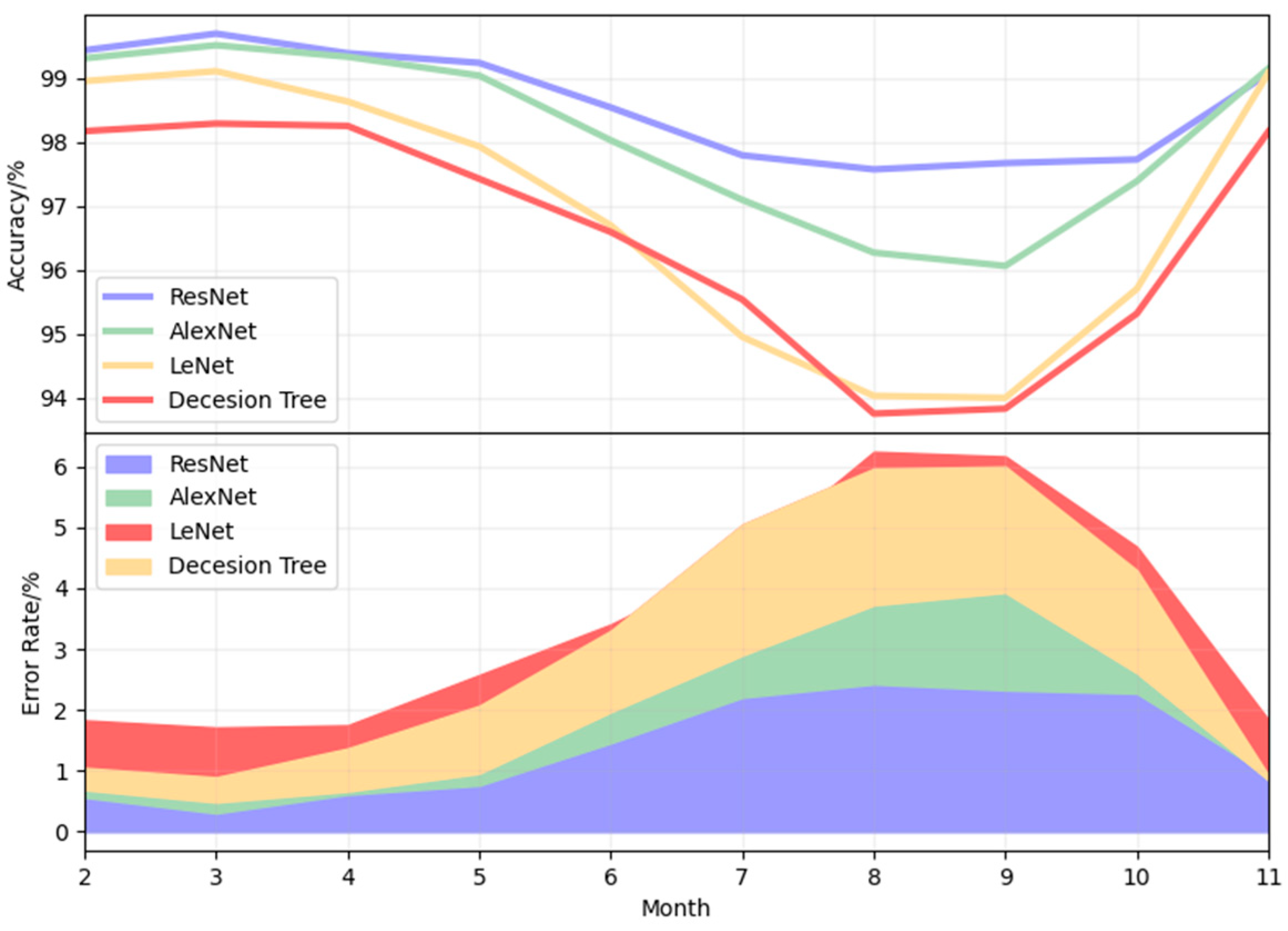
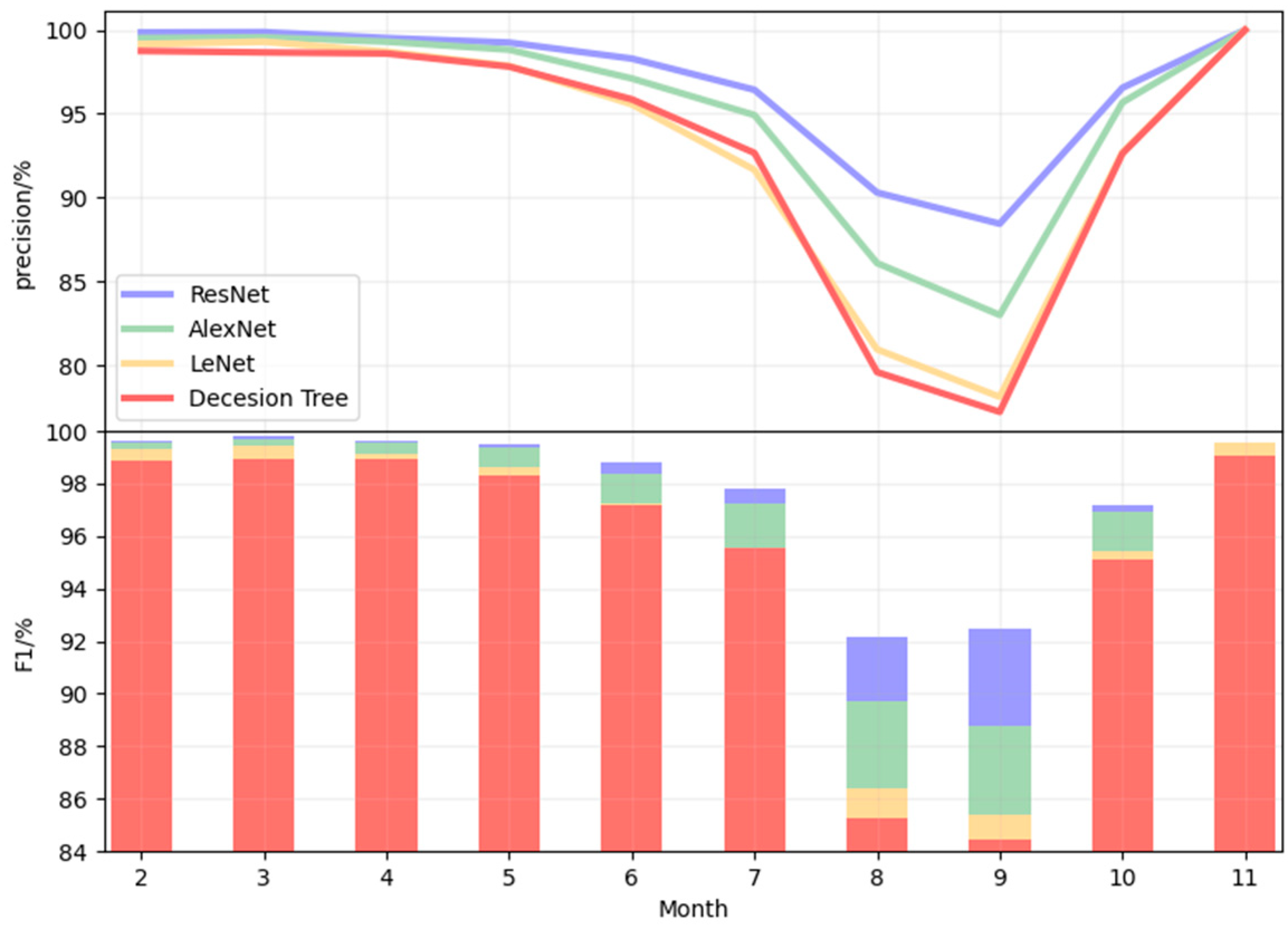
3.1. Results with Accuracy

To highlight the advantages of ResNet over other neural network structures, this paper compares ResNet with several other sea ice detection algorithms. We trained and tested the sea ice detection-oriented methods using the same DDMs described above, and the results are presented in

Table 1. Monthly DDM count and accuracy of four algorithms for sea ice detection.

Month	Number of DDM	Accuracy
		AlexNet	Decision Tree	LeNet	ResNet
February	209,829	99.31%	98.20%	98.88%	99.43%
March	166,202	99.51%	98.34%	99.14%	99.69%
April	260,209	99.33%	98.27%	98.81%	99.38%
May	59,479	99.04%	97.50%	98.09%	99.23%
June	75,772	97.53%	96.62%	97.06%	98.53%
July	124,263	96.19%	95.67%	95.17%	97.79%
August	43,023	95.11%	93.82%	93.73%	97.57%
September	48,837	94.53%	93.85%	93.52%	97.67%
October	66,462	96.56%	95.52%	95.58%	97.73%
November	70,805	99.08%	98.14%	99.06%	99.06%
AVG		97.62%	96.59%	96.90%	98.61%

and

Table 2. Performance metrics of different algorithms for sea ice detection.

	Accuracy	Error Rate	Precision	F1-Score	Water_acc	Ice_acc
AlexNet	97.62%	2.38%	95.39%	96.87%	92.94%	99.30%
Decision Tree	96.59%	3.41%	93.17%	95.16%	90.23%	98.69%
Lenet	96.90%	3.10%	93.39%	95.56%	90.45%	99.13%
ResNet18	98.61%	1.39%	96.85%	97.63%	96.22%	99.13%

.

As shown in Table 1, the AlexNet model has a classification accuracy of 97.62%, the Decision Tree model achieves 96.59%, the Lenet model has an accuracy of 96.90%, and the ResNet model performs best with a 98.61% accuracy rate. ResNet-based sea ice detection model shows overall improved accuracy compared to other algorithms. The monthly average accuracy given in Table 1 is used to create line graphs illustrating the accuracy of sea ice detection across the four methods (see Figure 8).

Figure 8 illustrates the detection performance of each algorithm for various months and presents a clear trend in sea ice detection accuracy. The accuracy of the four algorithms shows a downward trend from May to September. Among the four methods, the accuracy of LeNet, AlexNet, and Decision Tree declines significantly, while ResNet only hs a slight decline, and from July to September, it tends to be stable. Compared with the other three methods, ResNet has higher and more stable accuracy. The lower panel in Figure 8 shows the area plot of error rates for the four algorithms, which clearly shows that the Decision Tree has the highest error rate while ResNet has the lowest error rate, showing better stability during sea ice melt compared to the other algorithms.

Table 2 presents a comprehensive overview of the detection results, encompassing accuracy, error rate, precision, F1-score, and the accuracy of both seawater and sea ice detection. From Table 2, it is evident that the accuracy of sea ice detection surpasses that of seawater detection for each algorithm. This discrepancy can primarily be attributed to the higher susceptibility of seawater DDMs to noise, consequently leading to the reduced seawater detection accuracy.

The Decision Tree algorithm demonstrates an accuracy of 96.59%, with seawater detection accuracy at 90.23% and sea ice detection accuracy at 98.69%. Compared to other types of convolutional neural networks, it exhibits the lowest overall accuracy. The LeNet network achieves a detection accuracy of 96.90%, with seawater detection accuracy at 90.45% and sea ice detection accuracy at 99.13%. On the other hand, AlexNet attains a detection accuracy of 97.62%, with seawater detection accuracy at 92.94% and sea ice detection accuracy at 99.30%. Remarkably, ResNet outperforms the other algorithms, registering a detection accuracy of 98.61%. Its seawater detection accuracy stands at 96.22%, and its sea ice detection accuracy is at 99.13%.

In conclusion, the complexity of the network model positively correlates with detection accuracy, with ResNet exhibiting the highest overall accuracy and the lowest error rate among the evaluated algorithms.

In comparing between seawater accuracy and sea ice accuracy based on the results given in Table 2 (see Figure 9), it is evident that the Decision Tree algorithm has the lowest accuracy in both seawater detection and sea ice detection compared with several convolutional neural networks. The expressions for these indicators are as follows:

$$\begin{array}{l}Accuracy=\frac{TP+TN}{TP+FN+FP+TN}\\ \mathrm{Pr}ecision=\frac{TP}{TP+FP}\\ \mathrm{Re}call=\frac{TP}{TP+FN}\\ F1-score=\frac{2\ast (\mathrm{Pr}ecision\ast \mathrm{Re}call)}{\mathrm{Pr}ecision+\mathrm{Re}call}\end{array}$$

(10)

• True Positive (TP): the prediction is positive and the result is correct.
• False Positive (FP): the prediction is positive and the predicted result is incorrect.
• True Negative (TN): the prediction is negative and the predicted result is correct.
• False Negative (FN): the prediction is negative and the result is wrong.

Among the three CNNs, LeNet has the lowest accuracy in detecting seawater, showing the worst performance. Although the AlexNet has the highest accuracy in detecting sea ice, it lacks precision in detecting seawater, resulting in a significant decline in accuracy during the melting period from June to September. ResNet has the same sea ice detection accuracy as AlexNet, but the detection rate of seawater is much higher than other algorithms, which is the reason why it shows better stability during the sea ice melting period. Therefore, during the melting period, the accuracy of ResNet is more stable, with an average accuracy of up to 98.61%, which is the best among the tested methods.

Figure 10 shows the line chart for precision and the F1-score histogram based on Table 2. Precision is concerned with the accuracy of the model predicting positive cases. A high precision rate means that the model predicts few false positives among the positive cases. Recall, on the other hand, focuses on the model’s ability to capture and correctly predict all instances of a positive class within a dataset. F1 scores combine precision and recall performance, and are more stable on unbalanced data sets because they take into account both the prediction accuracy and coverage of the model. ResNet has the highest precision and F1-score among all four algorithms from February to November, proving the algorithm’s superiority in terms of sea ice detection.

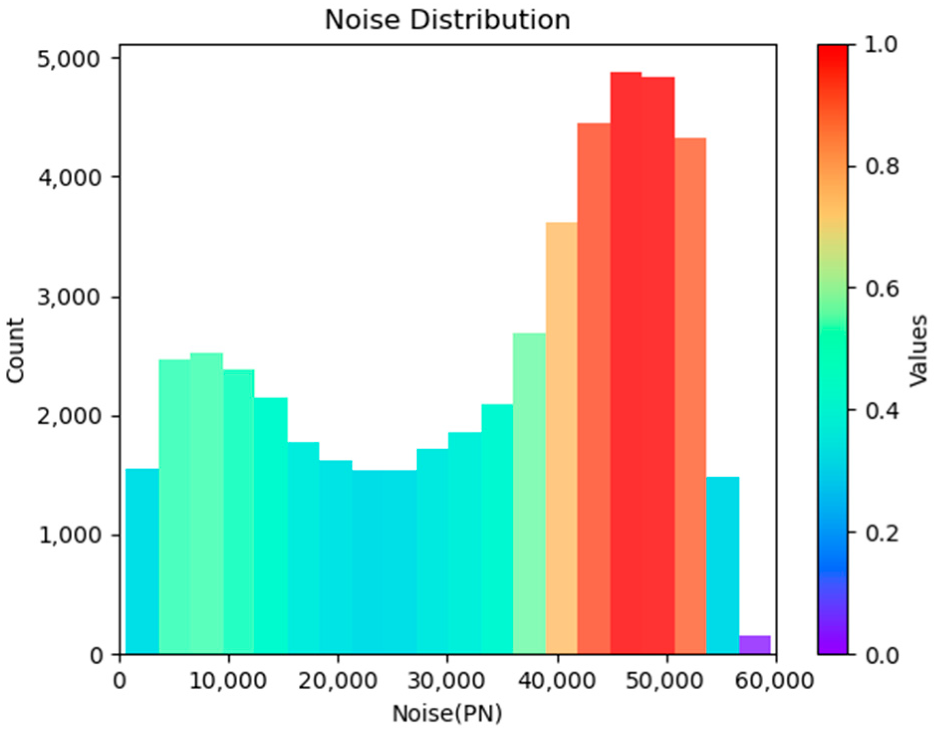
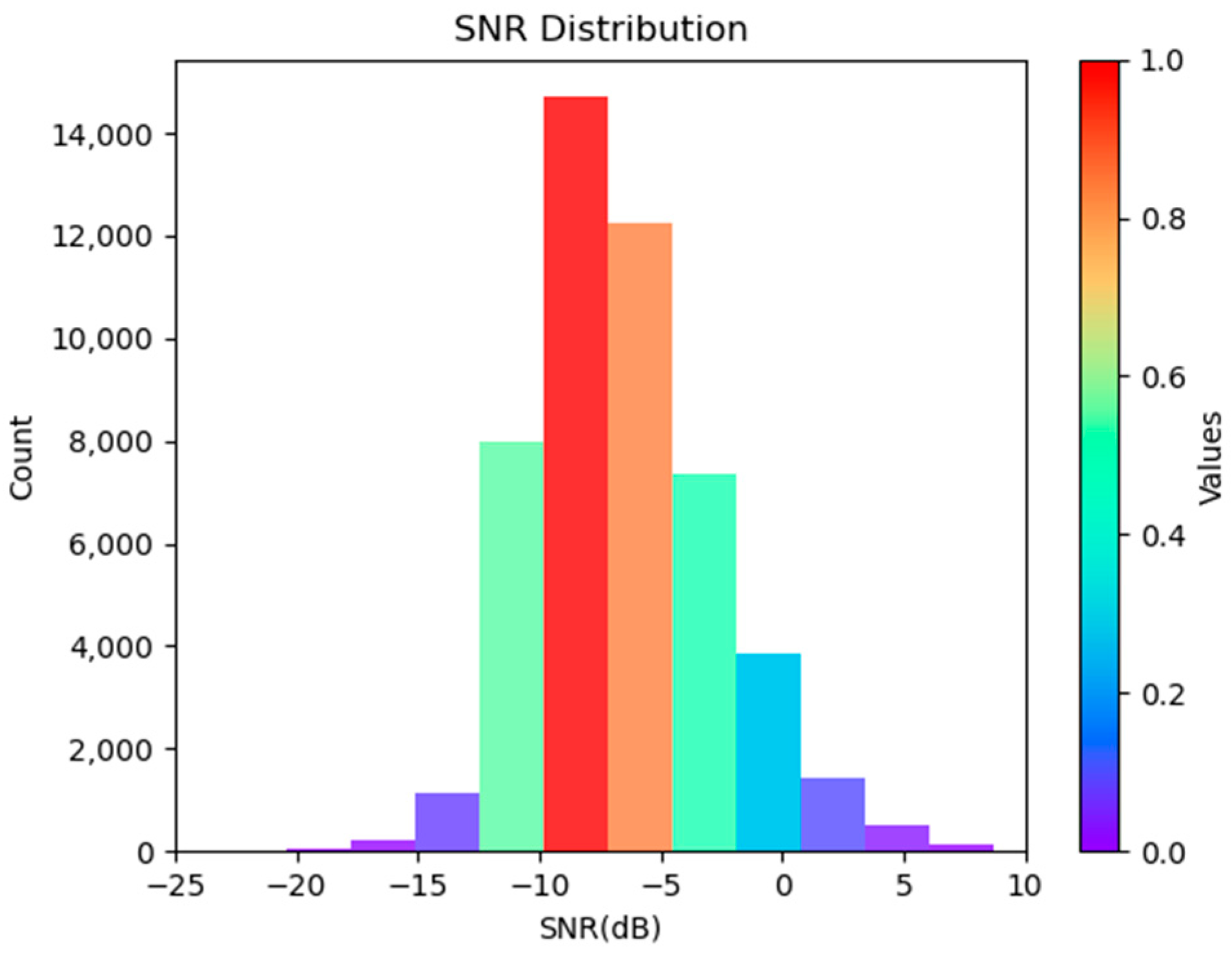
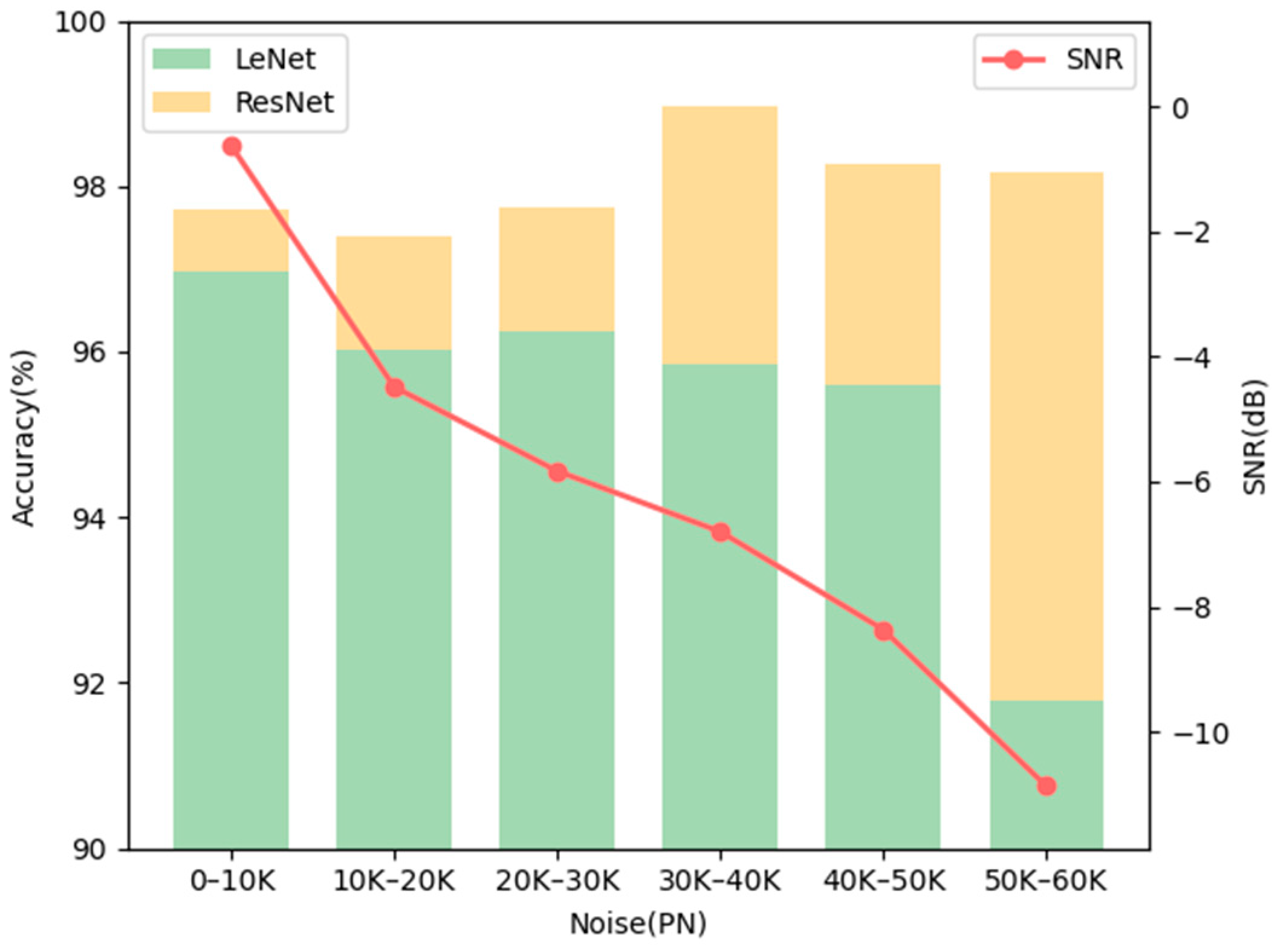
3.2. Analysis in Relation to Accuracy, SNR, and Noise

The noise and SNR of DDMs have a great impact on the accuracy of sea ice detection. The above results show that the sea ice detection accuracy for the whole year reaches its lowest point in September, so the DDM for September is selected for analysis. Figure 11 and Figure 12 show the distribution of noise and SNR for the September dataset. The range of noise is between 0 and 60,000 PN, with relatively more data in the range of 40,000–55,000 PN, which shows that the majority of the data is affected by noise. The range of SNR is between −25 and 10 dB, with a relative concentration of −10 to −5 dB.

Based on the magnitude of noise, this study classifies the DDMs into different categories. The range of 0–60,000 PN is divided into six segments, each corresponding to a distinct noise level. As illustrated in Figure 13, the average SNR of DDMs decreases with increasing noise, indicating that higher noise levels lead to more severe interference and adversely affect the accuracy of sea ice detection.

By comparing the performance of LeNet and ResNet in different noise segments for sea ice detection, it can be observed that when using LeNet for sea ice detection, the SNR decreases with increasing noise, and consequently, the accuracy of sea ice detection diminishes. It is worth noting that, at 50,000–60,000 PN, the sea ice detection accuracy exhibits a sharp decline. In contrast, the ResNet algorithm appears less sensitive to variations in noise and SNR, displaying stable performance.

This observation suggests that ResNet exhibits consistent accuracy despite changes in noise levels, while LeNet’s detection accuracy is adversely impacted by increasing noise levels, resulting in diminished performance.

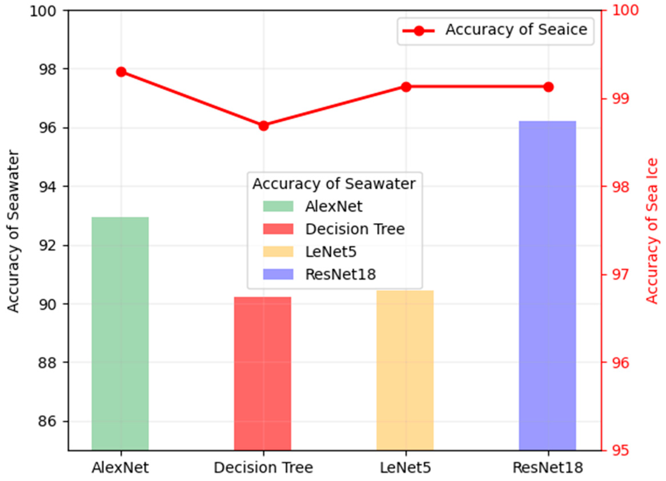
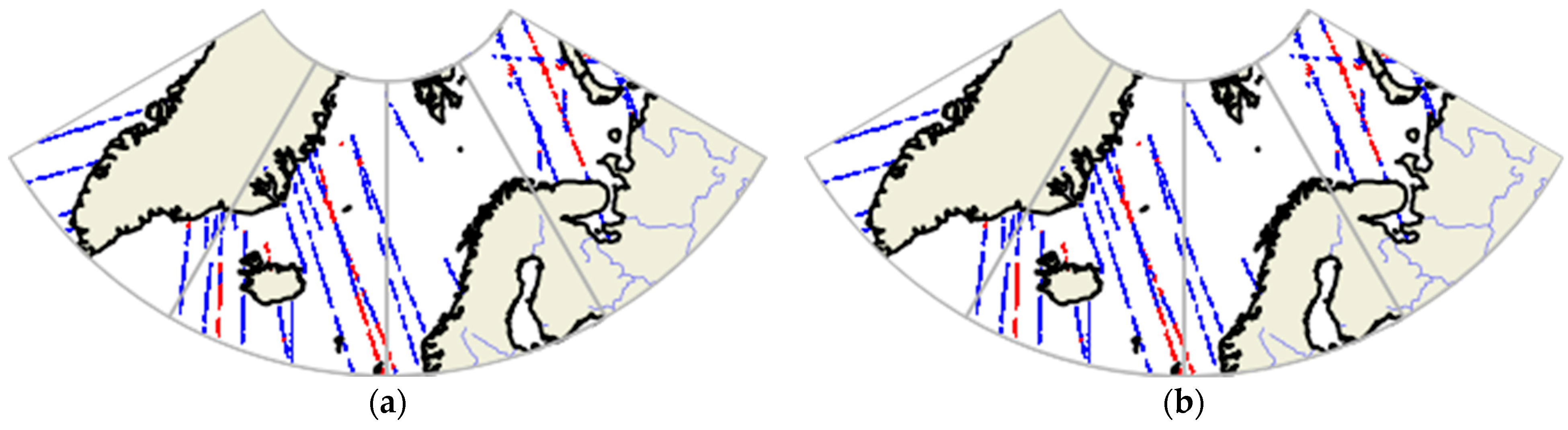
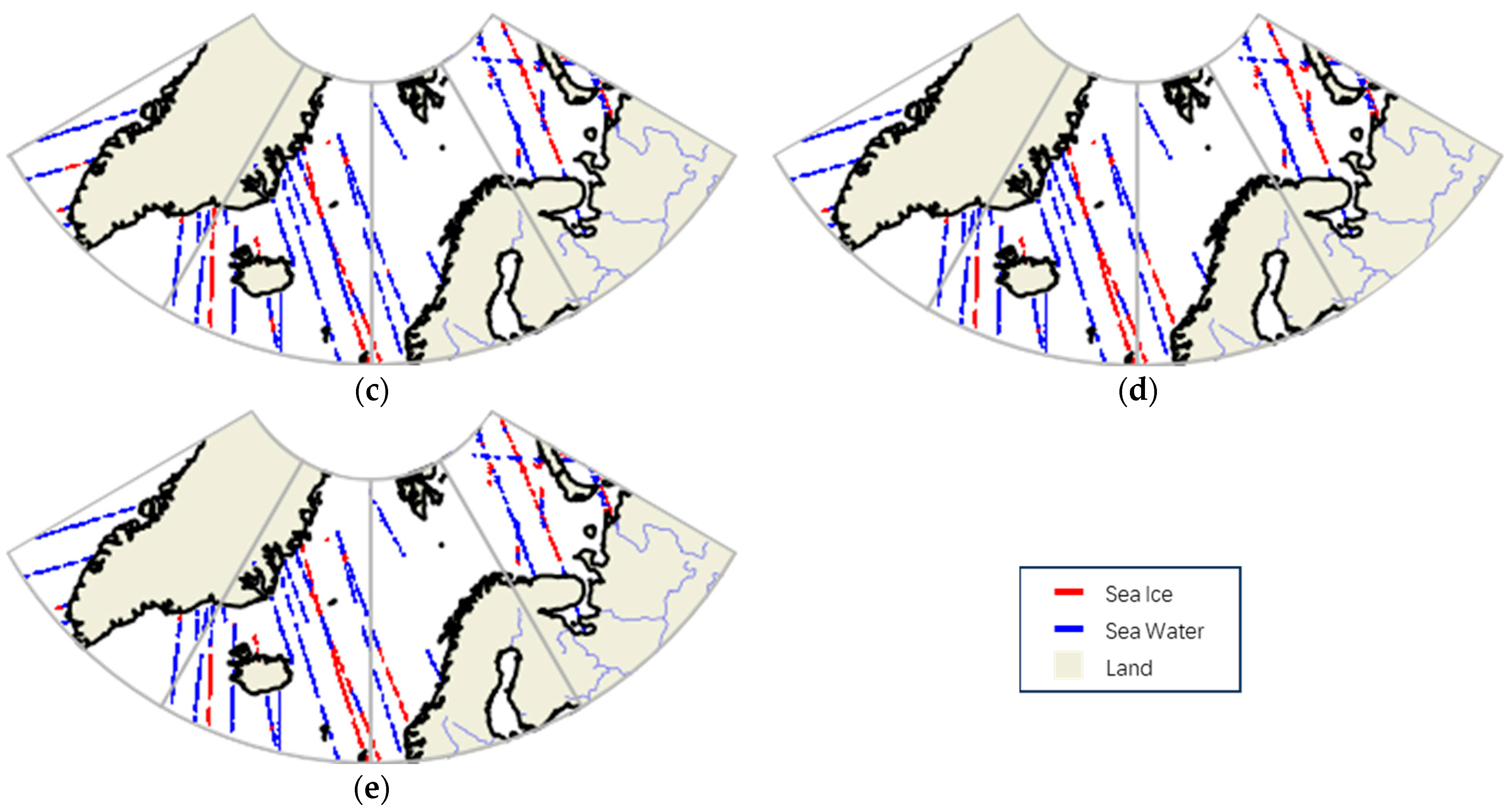
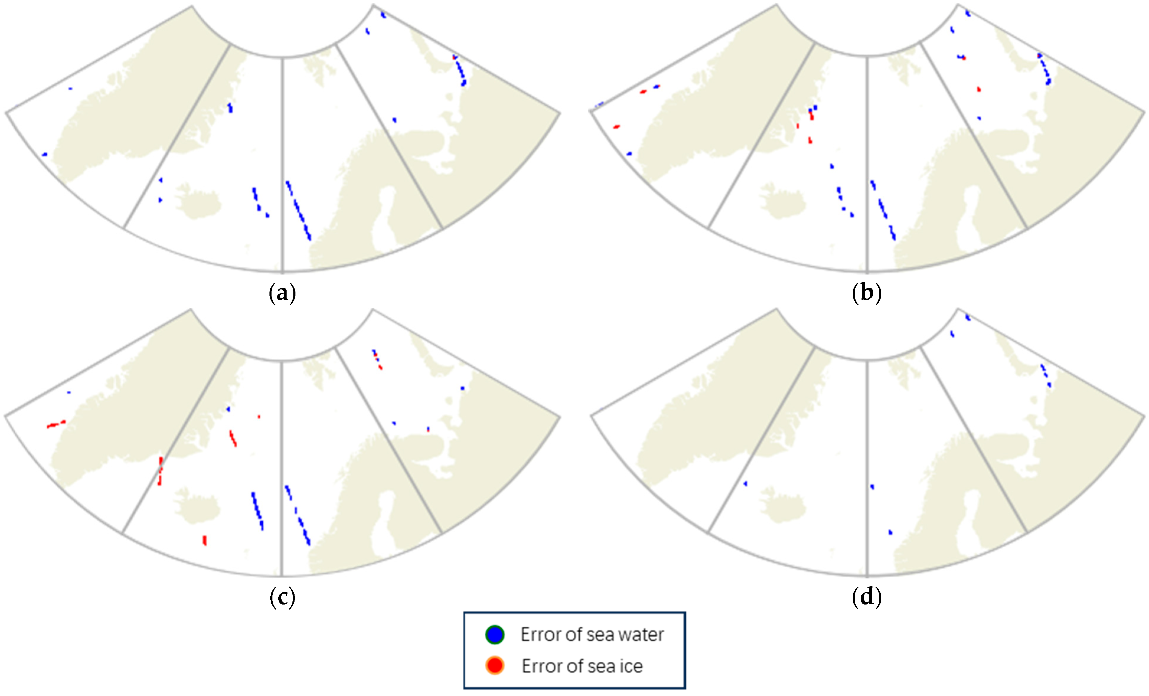
3.3. Analysis in Relation to Ground Truth

For analyzing the consistency of the GNSS-R sea ice detection algorithm with NOAA data, this paper analyzes the correlation between NOAA surface type data and the results of each sea ice detection, and draws the comparison between the prediction results and the real values of the ground truth. The mapping area was selected around Greenland, Iceland and Norway. Sea ice off Greenland is key in global climate change studies, reflecting the climate dynamics of the Arctic region. Iceland is located south of the Arctic Circle, and its sea area is also influenced by the Arctic Ocean, with the sea ice in the vicinity showing seasonal changes. The northern waters of Norway are also a key ice area, especially in winter. Thick, multi-year ice cover may exist in north-west Iceland and around the Svalbard archipelago in Norway. With seasonal changes, sea ice in these areas undergoes significant expansion and contraction, affecting the climate and ecosystems of the surrounding seas.

The prediction results and the ground truth on 25 September 2018 are selected as shown in Figure 14, where red denotes seawater, blue denotes sea ice, and grey denotes land. In Figure 14a–d, the sea ice detection results are represented from the four algorithms AlexNet, Decision Tree, LeNet, and ResNet, respectively, and Figure 14e represents the ground truth value. From Figure 14, it can be seen that the prediction results of the ResNet are closest to the ground truth.

To visualize the results of the sea ice detection of each algorithm, this paper also draws an error map as shown in Figure 15. The error points of the four algorithms are derived by comparing each prediction result with the real value, where blue indicates the seawater prediction error and red indicates the sea ice prediction error. From Figure 15, it can be seen that the ResNet-based sea ice detection has the least number of error points.

Detailed sea ice detection accuracy, seawater detection accuracy, and number of prediction errors are given in

Table 3. Sea ice detection results using different methods on 25 September 2018.

	Number of DDMs	Number of Errors	Accuracy	Error Rate	Water_acc	Ice_acc
AlexNet	12,935	700	94.64%	5.36%	81.25%	99.41%
Decision Tree	12,935	1124	91.33%	8.67%	83.88%	93.63%
Lenet	12,935	1201	90.86%	9.14%	85.45%	92.76%
ResNet18	12,935	58	99.50%	0.5%	98.41%	99.99%

, from which it is evident that most prediction errors arise from seawater DDM predictions. This aligns with the lower accuracy observed in seawater detection compared to sea ice detection, as indicated in the table. Seawater DDMs are more susceptible to noise, leading to classification errors and decreased detection accuracy. Another contributing factor is that during September, a period of sea ice melting, many ice fragments appear as floating ice, causing DDM features to fall between sea ice and seawater, resulting in prediction errors. Therefore, improving sea ice detection requires considering these factors to enhance the robustness and accuracy of detection algorithms.

In comparing sea ice detection errors among various algorithms, ResNet exhibits the fewest errors. ResNet’s unique residual block structure makes it less sensitive to noise, significantly reducing the impact of noise on seawater DDMs and ensuring stable sea ice detection accuracy during the melting period, avoiding accuracy degradation seen in other algorithms.

4. Conclusions

This paper applies the ResNet algorithm to detect sea ice using DDM data from TDS-1. The results show that the accuracy of ResNet sea ice detection reaches 98.61% when tested on 2018 data, and the accuracy can be stabilized above 97.67% even in the melting period. Compared with the other three sea ice detection algorithms, ResNet significantly outperforms them, and its advantage is reflected in three respects: it achieves an overall improvement in accuracy; additionally, it shows better robustness to noise, consequently amplifying the accuracy of sea ice detection; furthermore, while alternative algorithms experience a decline in accuracy during the melting phase, ResNet consistently upholds its high accuracy, showcasing remarkable stability. The quality of DDMs is very important for sea ice detection, and DDM data contains noise. Nowadays, there is increasing research on denoising DDM data, and the method used in this paper to remove the underlying noise of DDMs is not the most effective method. Further work on DDM denoising methods remains necessary to obtain higher quality DDM data. The high sensitivity of the GNSS-R signal to the surface scattering characteristics of different ice types also provides research opportunities into sea ice type classification and sea ice thickness inversion.

References

1. Rothrock, D.A.; Yu, Y.; Maykut, G.A. Thinning of the Arctic Sea-Ice Cover. Geophys. Res. Lett. 1999, 26, 3469–3472. [Google Scholar] [CrossRef]
2. Klein, L.; Swift, C. An Improved Model for the Dielectric Constant of Sea Water at Microwave Frequencies. IEEE Trans. Antennas Propag. 1977, 25, 104–111. [Google Scholar] [CrossRef]
3. Tsang, L.; Newton, R.W. Microwave Emissions from Soils with Rough Surfaces. J. Geophys. Res. 1982, 87, 9017. [Google Scholar] [CrossRef]
4. Hall, C.D.; Cordey, R.A. Multistatic Scatterometry. In Proceedings of the International Geoscience and Remote Sensing Symposium, “Remote Sensing: Moving Toward the 21st Century”, Edinburgh, UK, 12–16 September 1988; IEEE: Piscataway, NJ, USA, 1988; Volume 1, pp. 561–562. [Google Scholar]
5. Guo, W.; Du, H.; Guo, C.; Southwell, B.J.; Cheong, J.W.; Dempster, A.G. Dempster Information Fusion for GNSS-R Wind Speed Retrieval Using Statistically Modified Convolutional Neural Network. Remote Sens. Environ. 2022, 272, 112934. [Google Scholar] [CrossRef]
6. Asgarimehr, M.; Arnold, C.; Weigel, T.; Ruf, C.; Wickert, J. GNSS Reflectometry Global Ocean Wind Speed Using Deep Learning: Development and Assessment of CyGNSSnet. Remote Sens. Environ. 2022, 269, 112801. [Google Scholar] [CrossRef]
7. Guo, W.; Du, H.; Cheong, J.W.; Southwell, B.J.; Dempster, A.G. Dempster GNSS-R Wind Speed Retrieval of Sea Surface Based on Particle Swarm Optimization Algorithm. IEEE Trans. Geosci. Remote Sens. 2022, 60, 4202414. [Google Scholar]
8. Asgarimehr, M.; Zhelavskaya, I.; Foti, G.; Reich, S.; Wickert, J. A GNSS-R Geophysical Model Function: Machine Learning for Wind Speed Retrievals. IEEE Geosci. Remote Sens. Lett. 2020, 17, 1333–1337. [Google Scholar] [CrossRef]
9. Yan, Q.; Huang, W.; Jin, S.; Jia, Y. Pan-Tropical Soil Moisture Mapping Based on a Three-Layer Model from CYGNSS GNSS-R Data. Remote Sens. Environ. 2020, 247, 111944. [Google Scholar] [CrossRef]
10. Yan, Q.; Gong, S.; Jin, S.; Huang, W.; Zhang, C. Near Real-Time Soil Moisture in China Retrieved From CyGNSS Reflectivity. IEEE Geosci. Remote Sens. Lett. 2022, 19, 8004205. [Google Scholar] [CrossRef]
11. Yang, T.; Wan, W.; Sun, Z.; Liu, B.; Li, S.; Chen, X. Comprehensive Evaluation of Using TechDemoSat-1 and CYGNSS Data to Estimate Soil Moisture over Mainland China. Remote Sens. 2020, 12, 1699. [Google Scholar] [CrossRef]
12. Santi, E.; Paloscia, S.; Pettinato, S.; Fontanelli, G.; Clarizia, M.P.; Comite, D.; Dente, L.; Guerriero, L.; Pierdicca, N.; Floury, N. Remote Sensing of Forest Biomass Using GNSS Reflectometry. IEEE J. Sel. Top. Appl. Earth Obs. Remote Sens. 2020, 13, 2351–2368. [Google Scholar] [CrossRef]
13. Yan, Q.; Chen, Y.; Jin, S.; Liu, S.; Jia, Y.; Zhen, Y.; Chen, T.; Huang, W. Inland Water Mapping Based on GA-LinkNet From CyGNSS Data. IEEE Geosci. Remote Sens. Lett. 2023, 20, 1500305. [Google Scholar] [CrossRef]
14. Ghiasi, Y.; Duguay, C.R.; Murfitt, J.; van der Sanden, J.J.; Thompson, A.; Drouin, H.; Prévost, C. Application of GNSS Interferometric Reflectometry for the Estimation of Lake Ice Thickness. Remote Sens. 2020, 12, 2721. [Google Scholar] [CrossRef]
15. Yan, Q.; Huang, W.; Foti, G. Quantification of the Relationship Between Sea Surface Roughness and the Size of the Glistening Zone for GNSS-R. IEEE Geosci. Remote Sens. Lett. 2018, 15, 237–241. [Google Scholar] [CrossRef]
16. Yan, Q.; Huang, W. Spaceborne GNSS-R Sea Ice Detection Using Delay-Doppler Maps: First Results From the U.K. TechDemoSat-1 Mission. IEEE J. Sel. Top. Appl. Earth Obs. Remote Sens. 2016, 9, 4795–4801. [Google Scholar] [CrossRef]
17. Zhu, Y.; Yu, K.; Zou, J.; Wickert, J. Sea Ice Detection Based on Differential Delay-Doppler Maps from UK TechDemoSat-1. Sensors 2017, 17, 1614. [Google Scholar] [CrossRef]
18. Alonso-Arroyo, A.; Zavorotny, V.U.; Camps, A. Sea Ice Detection Using, U.K. TDS-1 GNSS-R Data. IEEE Trans. Geosci. Remote Sens. 2017, 55, 4989–5001. [Google Scholar] [CrossRef]
19. Yan, Q.; Huang, W.; Moloney, C. Neural Networks Based Sea Ice Detection and Concentration Retrieval From GNSS-R Delay-Doppler Maps. IEEE J. Sel. Top. Appl. Earth Obs. Remote Sens. 2017, 10, 3789–3798. [Google Scholar] [CrossRef]
20. Yan, Q.; Huang, W. Sea Ice Sensing From GNSS-R Data Using Convolutional Neural Networks. IEEE Geosci. Remote Sens. Lett. 2018, 15, 1510–1514. [Google Scholar] [CrossRef]
21. Yan, Q.; Huang, W. Detecting Sea Ice From TechDemoSat-1 Data Using Support Vector Machines With Feature Selection. IEEE J. Sel. Top. Appl. Earth Obs. Remote Sens. 2019, 12, 1409–1416. [Google Scholar] [CrossRef]
22. Hu, Y.; Jiang, Z.; Liu, W.; Yuan, X.; Hu, Q.; Wickert, J. GNSS-R Sea Ice Detection Based on Linear Discriminant Analysis. IEEE Trans. Geosci. Remote Sens. 2023, 61, 5800812. [Google Scholar] [CrossRef]
23. He, K.; Zhang, X.; Ren, S.; Sun, J. Deep Residual Learning for Image Recognition. In Proceedings of the IEEE Conference on Computer Vision and Pattern Recognition CVPR, Boston, MA, USA, 7–12 June 2015. [Google Scholar]
24. Zavorotny, V.U.; Voronovich, A.G. Scattering of GPS Signals from the Ocean with Wind Remote Sensing Application. IEEE Trans. Geosci. Remote Sens. 2000, 38, 951–964. [Google Scholar] [CrossRef]
25. Yan, Q.; Huang, W. Sea Ice Remote Sensing Using GNSS-R: A Review. Remote Sens. 2019, 11, 2565. [Google Scholar] [CrossRef]
26. Al-Khaldi, M.M.; Johnson, J.T.; Gleason, S.; Loria, E.; O’Brien, A.J.; Yi, Y. An Algorithm for Detecting Coherence in Cyclone Global Navigation Satellite System Mission Level-1 Delay-Doppler Maps. IEEE Trans. Geosci. Remote Sens. 2021, 59, 4454–4463. [Google Scholar] [CrossRef]
27. Kingma, D.P.; Ba, J. Adam: A Method for Stochastic Optimization. arXiv 2017, arXiv:1412.6980. [Google Scholar]
Figure 1. DDMs collected by TDS-1: (a) seawater DDM; (b) sea ice DDM.
Remotesensing 15 04477 g001
Figure 2. Error-prone DDMs in sea ice detection: (a) aeawater DDM affected by noise; (b) sea ice DDM affected by noise; and (c) sea ice DDM during melting period.
Remotesensing 15 04477 g002
Figure 3. Convolutional neural network module: (a) baseline; (b) ResNet.
Remotesensing 15 04477 g003
Figure 4. Employed Structure of ResNet in this paper.
Remotesensing 15 04477 g004
Figure 5. Residual module: a straightforward residual block.
Remotesensing 15 04477 g005
Figure 6. Employed structure in this paper: (a) structure of LeNet; and (b) structure of AlexNet.
Remotesensing 15 04477 g006
Figure 7. A flowchart of sea ice detection.
Remotesensing 15 04477 g007
Figure 8. Accuracy and error rate of seasonal sea ice detection from February to November.
Remotesensing 15 04477 g008
Figure 9. Comparison of detection accuracy: seawater and sea ice.
Remotesensing 15 04477 g009
Figure 10. F1 Score and precision of sea ice detection from February to November.
Remotesensing 15 04477 g010
Figure 11. Noise distribution in September.
Remotesensing 15 04477 g011
Figure 12. SNR distribution in September.
Remotesensing 15 04477 g012
Figure 13. SNR and sea ice detection accuracy corresponding to DDMs in different noise segments.
Remotesensing 15 04477 g013
Figure 14. Results of sea ice detection using different methods on 25 September 2018: (a) AlexNet, (b) Decision Tree, (c) LeNet, (d) ResNet, and (e) ground truth.
Remotesensing 15 04477 g014aRemotesensing 15 04477 g014b
Figure 15. Errors of sea ice detection results using different methods on 25 September 2018: (a) AlexNet, (b) Decision Tree, (c) LeNet, and (d) ResNet.
Remotesensing 15 04477 g015