Abstract
Proximity remote sensing techniques, both land- and drone-based, allow for a significant improvement of the quality and quantity of raw data employed in the analysis of rockfall phenomena. In particular, the large amount of data these techniques can provide allows for the use of probabilistic approaches to rock mass characterization, with particular reference to block volume and shape definition. These, in return, are key parameters required for a proper rockfall hazard assessment and the optimization of countermeasures design. This study aims at providing a sort of guide, starting from the data gathering phase to the processing, up to the implementation of the outputs in a probabilistic-based scenario, which is able to associate a probability of not being exceeded with total kinetic energy values. By doing so, we were able to introduce a new approach for the choice of design parameters and the evaluation of the effectiveness of mitigation techniques. For this purpose, a suitable case study located in Varaita Valley (Cuneo, Italy) has been selected. The area has been surveyed, and a model of the slope and a digital model of the rock faces have been defined. The results show that a 6.5 m3 block has a probability of not being exceeded of 75%; subsequent simulations show that the level of kinetic energy involved in such a rockfall is extremely high. Some mitigation techniques are discussed.
1. Introduction
In the last decade, the use of photogrammetric techniques has seen a large spread, particularly in the geosciences, where they are highly useful at all scales of investigation to produce accurate, high-resolution digital models [1]. To be more specific, in the field of Rock Mechanics, such an approach has proven useful in producing digital models of rock masses and rock outcrops, from which geometrical features are to be extracted: i.e., discontinuity spacing, persistence and orientation derived from traces and planes, respectively [2,3,4,5,6,7,8]. It is also possible to extract the roughness of the discontinuity surfaces visible on the model, provided that this has a sufficiently high resolution [9]. Nowadays, the standard tools employed to produce a digital model of a rock face are terrestrial and drone-based photogrammetry, along with laser scanning techniques. These tools have proven to be more adaptable and more manageable than laser scanners; more importantly, the cost and accessibility requirements of photogrammetric techniques are lower, considering that the basic equipment consists of a digital camera and a personal computer (PC) for the processing phase. Even smartphones can be used for this purpose [10].
The introduction and widespread diffusion of small and manageable Unmanned Aerial Vehicles (UAVs) have increased the appeal of photogrammetric techniques, given the significant advantages a tool such as a UAV can provide. First of all, employing a UAV allows one to survey large areas in a relatively short amount of time, allowing for the definition of digital models of large and very large rockfaces, for example [11]. Another significant advantage, especially when compared to standard terrestrial photogrammetry and other terrestrial techniques, is related to the possibility one has of covering rockfaces in their full 3D complexity, an advantage made possible by the flying nature of the platform where the sensor is installed. For the same reason, it is also possible to employ drones to map sectors or rock masses even in positions that are difficult to access or impossible to reach [12]. This is also true for cases where the rock mass lies within reservations or protected areas, such as, for example, archeological sites [13].
Photogrammetry also plays an important role in matters such as landslide investigation and monitoring or hazard mapping. UAV-based techniques provide a cheap and high-resolution solution for the definition of the morphological parameters describing a slope [14] but also give important information required to define the numerical models, both 2D and 3D, commonly employed to quantify and then map the hazard produced by phenomena such as rockfall and then develop a proper mitigation approach [15,16,17]. In this regard, it is worth mentioning the fact that non-contact techniques for rock mass surveys have proven even more useful due to the high quantity of quality data they can provide, allowing for proper statistical treatment [18] and the use of probabilistic approaches. Among others, one with significant potential involves the definition of an In Situ Block Size Distribution (IBSD) [19,20,21,22]. This method employs a probability distribution to describe the possible values of block volume within a given rock mass as a function of the orientation and spacing distributions of its discontinuities: i.e., a proper description of its geometrical features, accounting also for the natural variation in these parameters. A proper, complete and statistically reliable description of block volume or size is a key step in the definition of the parameters describing the mechanical problem presented by rockfall processes: these are usually accounted for, especially when dealing with protective works, in terms of total kinetic energy, which is a function of the block velocity and its mass. The mass is, in return, a function of block volume and rock density.
A similar approach should also be employed when dealing with block shape. It is proven that the shape of a falling block significantly influences its possible trajectories and energies [18,23] or the interaction between the block itself and the vegetation it may encounter along its path downslope [24]. The literature is also rich in examples of methods for classifying block shapes [25,26] and tools and software that model rockfall dynamics accounting for block shape [27,28,29]. To the authors’ knowledge, though, in no case was a complete description and quantification of the possible shapes rock blocks can manifest presented and, more importantly, used to quantitatively assess the effects of block shape in a rockfall scenario. This appears to be a significant point, worthy of investigation.
In this paper, we present a complete methodology for assessing rockfall hazards, starting from the data-gathering phase up to the design of protection works. In this method, we approach both block size and shape from a probabilistic point of view, taking them both into account in the numerical simulations needed to define the hazard scenarios and to choose the proper protection works. Consequently, the outputs of the proposed procedure are also probabilistic: this fact represents an element of novelty, as it is standard practice to reduce this kind of analysis to deterministic descriptors of the problem. Therefore, our approach makes it possible to build a complete spectrum of design scenarios, among which the designer can choose the best one considering its effectiveness and costs.
A suitable case study was identified in the Western Italian Alps (Upper Varaita Valley, Piedmont Region, Northwestern Italy), in the municipality of Bellino. The area represents a typical alpine valley, with a wide valley bottom and steep or very steep slopes, generally carved into the bedrock. The study area is focused on a small cluster of old buildings, named Grangia Cruset, and the steep slope to its North. There, a large isolated rocky peak (Mt. Rocca Senghi) is visible, and the rock faces in its vicinity are recorded as rockfall sources by the Regional Landslide Inventory (SIFRAP) [30].
2. Materials and Methods
The work presented here is structured in three phases: data acquisition, data processing and interpretation and design, which will be called Phase 1, 2 and 3, respectively. Phase 1 corresponds to the gathering of raw data of the studied rockface: the aim here is to construct a digital model of the rockface itself by means of photogrammetric surveys, extract the geometrical features of the rock mass through non-contact technics and validate the results through traditional contact measurements performed at the toe of the rockface. Once Phase 1 is complete, the data obtained can be processed, and rockfall hazard can be evaluated (Phase 2): this is achieved by constructing the IBSD from the rock mass geometric data, evaluating the block shape distribution and identifying the source areas of possible rockfall events; consequently, these outputs are employed to properly define a realistic model upon which to implement both 2D and 3D numerical simulations of block trajectories, from which rockfall hazard can be assessed. Lastly, based on the information derived from Phase 2, a suitable and efficient mitigation strategy, as well as a proper design of protection works, can be implemented (Phase 3).
It is worth noting that the common denominator in all three phases is the underlying probabilistic methodology. This is highly important: as pointed out by Bourrer et al. [31], among others, the deterministic description of processes such as rockfall tends to highly oversimplify the problem due to the impossibility of properly describing every variable involved realistically, be it the topography of the slope, the rock mass features or the shape of blocks. Therefore, a probabilistic approach is strongly advised and feasible, considering how fast and simple it is to obtain through non-contact methods large quantities of high-quality raw data to be used for rock mass characterization.
The methodology and material employed in each of the three phases will be presented in separate sections.
2.1. Phase 1: Data Acquisition
Phase 1 consists of gathering sufficient raw data of good quality to perform a proper assessment of the features of a given rock mass, particularly in terms of the fracture network that generates the blocks. As raw data, we indicate here the unprocessed data gathered on the field. Figure 1 shows the Phase 1 workflow, distinguishing among input data (in blue), operations (in black) and output data (in green). These last ones will become the input data of Phase 2.
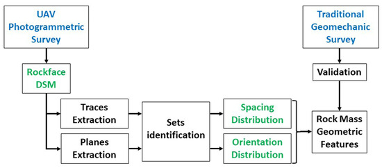
Figure 1.
Workflow of Phase 1: input data (blue) required by the process, operations (black) and output data (green) for Phase 2.
Non-contact survey methods for rock mass characterization have proliferated in the last decade [3,4,5,32,33,34,35,36], highlighting the advantages in terms of safety and time duration of the operations and allowing for the acquisition of large datasets. The data gathered by non-contact surveys need to be validated so that gross errors in set orientation are avoided. This is accomplished by comparing the results with measurements performed traditionally along the accessible portions of the rock face, using a compass and a scanline.
2.2. Phase 2: Data Processing
The processing of the data produced in Phase 1 is used to define three key characteristics of the studied rock mass: block volume, block shape and location of source areas of unstable blocks. Once they have been defined and identified, numerical simulations can be carried out. Details on these aspects will be provided in the following paragraphs.
2.2.1. Block Volume, Block Shape and Source Area Identification
Block kinetic energy is directly proportional to its mass, which in turn is directly proportional to its volume. Block size can be quantified through the use of different approaches, both deterministic and probabilistic. In this study, we follow the approach to block size description proposed by Lu & Latham (1999) [20], expanded in later works such as the one presented in Umili et al. (2023) [18]. In these works, the approach to the quantification of block size relies on probability distributions describing the spacing of the discontinuity sets identified in the rock mass: on their basis, the block volume distribution can be computed, employing the well-established Palmstrom’s formula [37]; this equation, which considers the block generated by the intersection of three discontinuity planes, is not geometrically proven and, actually, it tends to either underestimate or overestimate the block size, depending on the reciprocal orientation of the sets involved. A solution to this problem was recently found, and a new formulation was introduced [18]. Although apparently more complex than the one previously mentioned, this equation is geometrically proven and correctly estimates the block size. Applying the methodology described by Umili et al. (2023) [18], the IBSD can then be quantified. Both Palmstrom’s formula [38] and the new equation can be described as follows:
where Sp indicates the contribution provided by spacing, while Sh is the contribution of the block shape, i.e., that of the reciprocal orientation of the joint sets identified. It is worth mentioning that both Palmstrom’s expression and the new, geometrically proven one are only valid for three joint sets; a generalization of the algebraic equation for n joint sets is not yet available. To solve this issue, as mentioned in [18], a combinatory approach is suggested: if more than three joint sets are present in the analyzed rock mass, triplets of joint sets are selected, and the effect of their spacing distribution and orientation is quantified. Among all the outputs obtained in this manner, the most realistic one can be selected with reference to the field data gathered in Phase 1. This is also true for the block shape distribution assessment. It is important to mention that a clear advantage of the IBSD approach lies in the fact that the probabilistic description of block size provides a more complete vision of the problem: therefore, any choice made is intrinsically more reliable and, perhaps more importantly, backed by a rigorously determined quantitative description.
The block shape is an equally important parameter: the shape of a block influences how it moves downslope when involved in a rockfall, affecting the geometry of its trajectory and the tendency to roll rather than bounce. In some specific instances, it is even possible to witness rocks rolling upslope [23]. When implementing a probabilistic approach to block description, it is not sufficient to identify a representative block shape, but the analysis of the distribution of the shapes is required. This can be achieved following Umili et al. (2023) [18], where the authors present a way of assessing the real distribution of shapes associated with a given set of spacing probability density functions (pdf) and the derived IBSD. The output of this approach is the percentage of blocks pertaining to each of the four shape classes defined by Palmstrom (2001) [25]. In this way, it is possible to easily visualize the complex and articulated nature of any rock mass. Consequently, it is possible to choose one or more shapes to be considered in the trajectory simulations based on the rigid body method. It is worth mentioning that, as suggested by Umili et al. (2023) [18] and by other works analyzed there, a relation of sorts exists between the shape and size of rock blocks. In the present work, this concept is not treated, but we suggest referring to the cited research for more details.
To identify the source areas of potential rockfalls means to recognize those portions of the rockface where the detachment of the blocks is possible. Rock mass instability phenomena are generally classified according to four types of movement: Planar Sliding (PS), Tridimensional or Wedge Sliding (WS), Direct Toppling (DT) and Flexural Toppling (FT). The methods for verifying if one or more of these movements are kinematically possible are the well-known Markland’s Tests [39,40]: these tests assess if the geometrical configuration of the discontinuities within the rock mass and the orientation of the rockface, alongside the friction angle of the discontinuities, are compatible with the movement of blocks. The original version of the tests relies on stereographic projections and allows only for one rockface orientation to be tested at a time. A much more practical solution was proposed by Taboni et al. (2022) [37], who introduced an algorithm capable of performing Markland’s test requiring a DSM of the rockface and the geometric and mechanical features of the discontinuities. The advantage of this tool (named Automatic Markland’s Test Tool, AMTT) is clear: the complexity of the rockface geometry, which originally required the stereoplot tests to be replicated as many times as different orientations could be identified, is an overcome problem; the use of a DSM allows for inferring the orientation of the rockface in each of its points, the only limit being the spatial resolution and accuracy of the DSM itself. It should also be taken into account that, by definition, DSMs cannot reproduce hanging portions of a rock face; in this case, a traditional approach is still required. The tool, among other outputs, also maps the potential source areas of rockfall on the analyzed rockface. For the specific needs of this study, the AMTT tool will be used in its deterministic mode: in this case, the input data required to describe the discontinuities within the studied rock mass are simply the orientation and friction angle of each of the identified joint sets. The AMTT tool also requires two raster files describing the aspect and the slope of the investigated rockface, respectively. In the deterministic mode, the output files of the algorithm are four maps with the number of positive kinematic tests within each cell for each of the four types of movement, a map with the global number of positive kinematic tests for each cell and the map of source areas. The first set of maps is useful in identifying which areas are subjected to the different types of movement; the second map helps to identify which portions of the rockface are more potentially active; the last map identifies source areas as all cells where, at least once, a kinematic test has yielded positive results.
Figure 2 summarizes, in a workflow, this initial part of Phase 2.
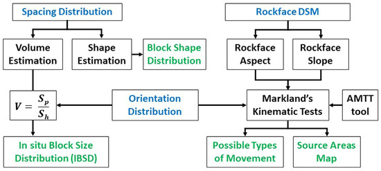
Figure 2.
Workflow detailing the definition of the IBSD, the block shape distribution and the identification of source areas (Phase 2); input data are in blue, operations in black and outputs in green.
2.2.2. 2D and 3D Rockfall Simulations
Once the block size, shape and source areas have been identified and properly described or quantified, numerical simulations can be performed. Two sets of simulations are presented in this paper: an initial 3D set and a more focused 2D one.
The 3D simulations have been performed using the raster-based Rockyfor3d software [27] aimed at mapping the runout and energetic features of the rockfall scenarios identified with respect to both the IBSD and block shape distribution. In this way, it is possible to recognize the most critical portions of the study area, on which the second set of numerical simulations is to be focused. Rockyfor3d maps many parameters: the number of passages per cell, kinetic energy and reach probability are only a small selection. The immediate usefulness of the last two parameters is self-evident, while the number of passages per cell can be used to identify preferential runoff paths, along which one can perform a deeper and more accurate analysis by employing 2D numerical simulations. The maps produced by Rockyfor3d are the base upon which to define the hazard scenarios of the study area. Considering the fact that the block shape distribution is to be accounted for, the following procedure is proposed: for each of the four possible shapes identified in Phase 2, a set of simulations is predisposed, the outcome of which will be weighted with reference to the relative abundance of each shape and then added together: this combination of partial outputs is defined by the following equation:
where SO indicates the global output of a given scenario, POe, POr, POs and POb represent the partial output for the equidimensional, rod-like, slab-like and blade-like shape, respectively, and e, r, s and b describe the relative abundance of the equidimensional, rod-like, slab-like and blade-like shape. This process needs to be replicated for every simulated volume derived from the IBSD. In fact, the approach just described can be applied only to the shape distribution, as it describes the relative abundance of the four different shapes by means of absolute frequencies; the same cannot be accomplished for the different volumes described by the IBSD, where each volume value is correlated to its probability of not being exceeded or to its cumulative frequency. It must be stressed how the evaluation of the shape distribution and its subsequent implementation in the numerical simulations is a methodological novelty introduced in this work. Although many software that are able to handle shapes exist, the use of the actual distribution of shapes to enhance the quality and accuracy of the results, as presented here, cannot be found anywhere else, to the authors’ knowledge. A schematic workflow describing these steps of Phase 2 is presented in Figure 3.
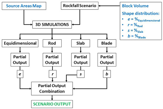
Figure 3.
Workflow detailing the approach employed for the 3D numerical simulations; input data are in blue, operations in black and outputs in green.
The last step of the data processing phase consists of the 2D numerical simulations, performed using a lumped mass software able to take an IBSD as the input data, such as Rocfall2 [41]. The topographic sections describe the preferential runout paths identified on the maps produced by Rockyfor3d and are directly extracted from the DSM of the study area. As mentioned, Rocfall2 allows for using as an input for the falling rock blocks a distribution of values, described in terms of the type of pdf, average value and standard deviation. These data are contained in the ISBD of the studied rock mass. Performing 2D simulations in this manner allows one to extract a probabilistic output. Therefore, the output of the 2D simulations allows for the construction of the kinetic energy probability distribution of any given point along the topographic section.
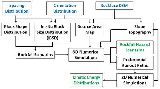
Figure 4 summarizes the entire Phase 2 as a workflow.
2.3. Phase 3: Interpretation and Design
By analyzing the maps obtained from the 3D numerical simulations, it is possible to derive a descriptor of the Rockfall Hazard of each portion of the study area. This can be accomplished by relying on the Reach Probability map provided as the output by Rockyfor3D. The software defines this quantity as follows [27]:
where Preach(x) is the reach probability of a given cell x, NB(x) is the number of blocks passing through the cell, Nsims is the number of simulations and Nsources(x) is the number of source cells from which a block reaches the considered cell. The map obtained in this manner describes the probability of a block reaching each cell of the analyzed area. By combining the contribution of each of the four shapes, as was carried out for each other output file of interest, it is possible to obtain a global map describing the tendency of falling blocks to reach each portion of the study area. By defining reasonable threshold values, it is possible to produce an easy-to-read map; in this study, the threshold values considered were:
- >10% = very high probability;
- 5–10% = high probability;
- 1–5% = moderate probability;
- <1% = low probability.
Although this map does not represent a true description of hazards due to the absence of the temporal distribution of the events of a given magnitude, it is still a very useful tool for identifying hazardous areas in a quantitative manner. With these scenarios available, and after the identification of the preferential runout paths in Phase 2, the design of mitigation and protection works is possible.
From the output of the 2D numerical simulations, a so-called Design Scenario can be defined; such a scenario can be visually described in terms of the energy of the phenomenon by a curve: the probability distribution of kinetic energy can be divided into portions, each of which identifies the range of effectiveness of a given passive or active countermeasure. In fact, the choice of a countermeasure directly depends on the energy involved in a given phenomenon, as that is the energy level it will be required to withstand; moreover, in the case of passive defensive works (i.e., embankments, flexible barriers), the structure has to be tall enough to capture the falling blocks. This means that the structure will have to be at least as high as the bounces those blocks produce along their path downslope. A probabilistic approach has the advantage of associating to each value a probability of not being exceeded, easily providing a well-structured and reliable method that avoids empirical choices of deterministic values but provides the full spectrum of possibilities. An example of a curve of the kind just described, named Design Scenario Curve (DSC), is visible in Figure 5. The curve is intended to be used in a twofold way: the first one consists of selecting a reference probability of not being exceeded on the vertical axis, intercepting the curve and identifying on the horizontal axis the correspondent parameter value (i.e., the kinetic energy in the figure). The second way, conversely, consists of entering a given parameter value on the horizontal axis (i.e., the kinetic energy, in the figure), intercepting the curve and quantifying the corresponding probability of not being exceeded. In the schematic diagram of Figure 5, we can see that two energy values are identified on the curve, corresponding to the maximum energy levels manageable by two types of mitigation techniques (active and passive): the Design Scenario allows one to visualize the effectiveness of a technique, based upon the extent of the portion of the DSC curve corresponding to energy values lower than the maximum service level of the technique. Everything above that level will require a different approach.
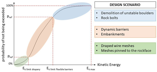
Figure 5.
Appearance of a generic DSC: the energy limits identified on the horizontal axis correspond to the maximum energy manageable by a given mitigation technique, described on the right.
A Design Scenario can be of great use for designers employing traditional and consolidated energy-based approaches: a DSC, in fact, describes the entire possible range of energy that a rockfall can potentially produce in a given context and, therefore, protection works have to account for. In other words, it is a quantitative and probabilistic description of the problem in its entirety. Here lies the innovation: instead of choosing a single, deterministic value for the key parameters required in the design phase, relying on empirical relations or heuristic methods, often overdependent on the professional experience of an individual, this choice can be justified purely in a quantitative way, relying on the robust and rigorous methodology underlying the results. In other words, the choice itself is not a matter of experience and subjectivity but of numbers and objective quantities. Similarly, the use of a probabilistic description of the key design parameters would prove significantly easier to regulate, as the lawmaker could define a minimum probability of not being exceeded to be used. Lastly, it is worth mentioning that a Design Scenario Curve can also function as input data for more sophisticated design approaches, such as those relying on the Reliability Analysis method [42,43,44].
Independent of the design approach employed, the first step always consists of the identification of the best site for the protection works: this choice has to take into account the falling rock’s trajectory, bounce height and kinetic energy. All these pieces of information can be derived from the 3D simulation outputs. The relative position of elements at risk also has to be accounted for: these data can be derived either from public databases or from the topographic survey performed in Phase 1. Once a suitable position has been identified, the distribution of values of kinetic energy and bounce height can be extracted from the 2D simulations; by calculating the cumulative frequency, it is possible to obtain a Cumulative Distribution Function (CDF), such as the one presented in Figure 5. The use of such a curve is, in the case of the kinetic energy one, as follows: with reference to the maximum energy value and the other issues related to the construction and installation of protection works (i.e., the value of the exposed buildings, logistic cost and feasibility, etc.), the designer is expected to choose one or more works; each of them will be certified as being efficient up to a certain energy level. By identifying that energy level on the curve, the designer can identify the correspondent probability of not being exceeded and its complementary probability of being exceeded, which in return provides an indication of the overall efficiency of the mitigation work. This can also be applied in the case of combined mitigation systems, where more than one solution is selected at once, as shown in Figure 5. A similar process is to be repeated with the bounces height distribution to define the height of the protection works, especially in the case of passive works such as flexible barriers or embankments. The key feature of this method lies in its quantitative nature: this is true both for the choice of the reference energy level to identify the best protection work and for the residual probability that is not mitigated by that structure.
3. Case Study
To test the methodology presented in the previous sections and to try out the effectiveness and efficiency of the workflow described, a suitable case study was identified in the Western Italian Alps (Upper Varaita Valley, Piedmont Region, Northwestern Italy), in the municipality of Bellino (province of Cuneo). The steep slope, including a large isolated rocky peak (Mt. Rocca Senghi), above a small cluster of old buildings named Grangia Cruset, is studied.
The area represents a typical glacial alpine valley, with a wide valley bottom currently occupied by a relatively small water stream, and steep or very steep slopes, generally carved into the bedrock. The slopes are widely affected by landslides, involving both the bedrock and the more recent sediment cover. This sector of the Upper Varaita Valley has an elevation beyond that of the vegetation, which is therefore mainly dominated by grass and very sparse larix trees. The geology of the area is dominated by metamorphic rocks, mainly quartzites and schists. These rocks appear heavily deformed, both with brittle and ductile behavior: this is recorded by the presence of both folds and faults. Consequently, the rock mass appears significantly fractured. A summary of the geographical, geomorphological and geological information regarding the case study area of Grangia Cruset is presented in Figure 6.
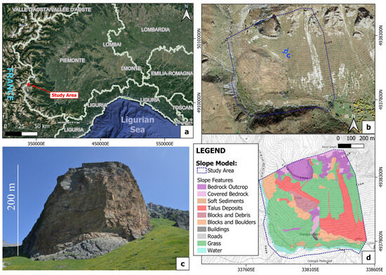
Figure 6.
(a) Location of the study area in the Western Italian Alps, (b) an aerial and (c) frontal view of the location and (d) the model of the slope features employed in the 3D simulations.
According to the Regional Landslide Inventory (SIFRAP) [30], the buildings of Grangia Cruset were hit in recent years by a large block detached from one of the rockfaces to the North. The event occurred on 22 July 2017: in total, a significant volume of rock of approximately 100 m3 detached from the peaks to the north of the location and fell towards the valley. Such a volume was most likely the result of different blocks detaching at the same time; moreover, these blocks fragmented into numerous smaller ones, with an average size ranging between 0.5 and 1.0 m3. Most notably, the largest intact block, with a volume of approximately 6.0 m3, ignored the local morphology: it rolled towards the buildings of Grangia Cruset, located on a small rise just above the main deposition area for rockfall, hitting the corner of one of them before proceeding towards the nearby water stream, where it stopped. The falling block caused only marginal damage to the building, but had it followed a different trajectory, it would have completely demolished any structure on its path. A small, flexible barrier has been installed not far from Grangia Cruset in the aftermath.
The slope to the north of Grangia Cruset is dominated by a large, isolated, rocky massif, located just southwest of Mt Rocca Senghi. This massif appears as the most likely source of rockfall in the area, alongside the smaller rockfaces to its east. Due to the special and interesting configuration of this peak, it has been chosen as the study subject of this paper: in fact, the area, in general, appears as a typical situation where the methodology presented in this paper could prove highly effective.
In this study, a photogrammetric survey of the investigated rockface was performed with a Parrot Anafi UAV. The rockface is more than 200 m high, almost vertically hanging over a slope whose steepness reaches 40 degrees in proximity to the rockface. Moreover, the shape of the rockface horizontal cross-section is almost circular. The need to reach a high altitude (about 2200 m asl) in order to acquire images of the whole rockface surface was required to be combined with the need to preserve the visual line of sight and fly the drone not higher than 120 m above the surface. These conditions, together with the variable wind conditions, made flight planning almost impossible and, therefore, the survey challenging. Images, whose resolution is 4608 × 3456 pixels, were shot through the manual control, keeping the focal length constant (4 mm, equivalent to 23 mm in a 35 mm full-frame sensor).
4. Results and Discussion
4.1. Phase 1
The image sequences obtained from the UAV flights were aligned by means of Agisoft Metashape, and the DSM of the rockface was obtained. The overall rockface area covered by the DSM is about 60,000 m2, and its average resolution is 40 points/m. The non-contact survey of discontinuity geometrical features (traces and planes) was performed on the DSM by means of the Rockscan code [45]. To validate these results, a series of traditional surveys was carried out on the rock mass itself. The discontinuities measured with both techniques are visible in the stereographic projection of Figure 7. Although with a certain variability, the studied rock mass features three main discontinuity sets (Table 1); among these, the one identified as K3 represents the main metamorphic foliation of the quartzite of the rock massif.
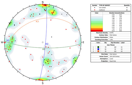
Figure 7.
Stereographic projection of the discontinuities measured through contact surveys (red dots) carried out along the sides of the rockface and through the analysis of the digital model of the rock mass (black dots). Three main sets of discontinuities are recognizable.

Table 1.
The three main discontinuity sets identified in the studied rock mass.
It is clear from Figure 7 that the data gathered on site, along scanlines located at the base of the rock face, and the data obtained from the digital model of the entire rock face are not perfectly matched. This is to be expected: as a consequence of where the traditional measurements were carried out, those data cannot be expected to completely describe a 200 m high rock face. To obtain a complete description would have required vertical scanlines to be carried out by a team of climbers. It is important to notice, though, that the two datasets are similar enough to convey the same information: the rock mass features three main sets of discontinuities, with reasonably clear orientations.
As can be observed from Table 1, the three sets clearly identify regular prismatic blocks, as the angles between them are always quite close to 90° (±20°). It should also be noted that the set identified as K1 is for all intents and purposes correspondent to the eastern-facing side of the rock mass, while K2 corresponds to its south-facing side. Other randomly oriented joints have been observed only in rare cases and can be considered, therefore, negligible for this work.
Regarding the spacing values, a statistical approach allowed for the quantitative choice of the best-fitting pdf for each set: details are visible in Table 2, in terms of the pdf type, mean value (μ) and variance (σ2).
Table 2.
Parameters of the best-fitting distributions of spacing samples.
4.2. Phase 2
Knowing the reference value of the orientation of each discontinuity set and their respective spacing distribution, it was possible to apply the methodology proposed by Umili et al. [18] and quantify the cumulative frequency distribution of the possible block volumes within the rock mass: namely, its IBSD (Figure 7).
The expected value (E[V]) and the variance (Var[V]) of the volume, under the assumption of constant Sh (E[Sh] = Sh, Var[Sh] = 0), can be explicitly calculated as follows [18]:
considering the spacing Si of the ith discontinuity set (i = 1, 2, 3) a continuous random variable, whose expected value and variance are μi and σi2, respectively.
The cumulative frequency corresponding to E[V], called F(E[V]), and the volume corresponding to 99% cumulative frequency in the IBSD, called V99%, can be adopted as descriptors of the IBSD [18]. Table 3 summarizes these data.
Table 3.
Uncertainty of the volume distribution and descriptors of the IBSD.
In this case, the probability of not being exceeded associated with the expected value of the volume is 80%, highlighting that the average volume does not necessarily correspond to the 50% probability of not being exceeded. V99% is a parameter describing the amplitude of the IBSD, truncated at 99% of cumulative frequency: in this case, it is equal to 70 m3, which is a realistic value in light of the recorded event.
As can be clearly seen in Figure 8, even for relatively low frequency values, the block size is significant. This fact is in line with the volume of the largest block involved in the event recorded on 22 July 2017, which, according to the IBSD, would have a frequency of approximately 74%. For convenience, for the following steps of Phase 2, we chose to rely on the block size corresponding to a frequency of 75%. This has a volume of 6.5 m3, just over the volume of the recorded event. From the three spacing distributions, the shape distribution can be derived: in Figure 9, a sample of one thousandblocks has been generated through a Monte Carlo simulation and classified. As can be seen, the most common types of blocks are the rod-like one (34%) and the slab-like one (30%), followed by the blade-like one (21%) and, lastly, the equidimensional or cubic one (15%).
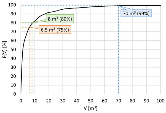
Figure 8.
IBSD of the studied rock mass with the volumes corresponding to 75%, 80% and 99% cumulative frequency F(V).
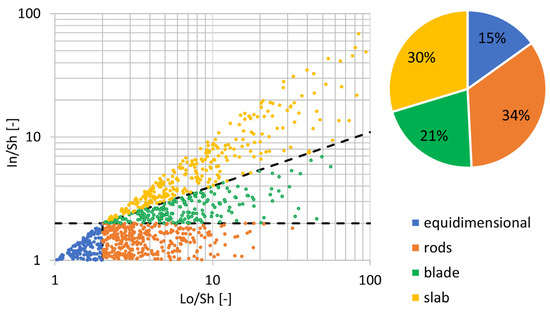
Figure 9.
Distribution of the four types of block shapes and their relative abundance.
Having selected the reference volume of 6.5 m3 and knowing the shape distribution, the 3D numerical simulations were performed. Rockyfor3d requires a set of ten grid files containing all the features of the slope, of the source area and of the blocks to be simulated. The features of the slope were derived from the model presented in Figure 6. A total of 10 types of surfaces were identified, ranging from water bodies to rocky outcrops, buildings and talus deposits and grass and dirt paths. From this surface classification, the soil type and roughness were defined according to the tables presented in the software manual. The slope was modeled by mapping out, both on-site and from satellite images, the distribution of the various types of surfaces; a map is visible in Figure 6. Ten classes were identified and are presented in the following Table 4 in terms of the soil type and equivalent normal restitution coefficient; this classification was carried out according to the approach described in Rockyfor3d’s manual [27].
Table 4.
The ten classes of soils and surfaces identified on the slope of the chase study area, their soil type and the range of normal restitution coefficient (Rn) values, as presented in the software’s manual [27].
To identify the source area, the AMTT tool [37] was used: this algorithm requires the reference orientation values for each of the three discontinuity sets, the slope angle and the aspect angle of the considered rock face. These two values were extracted from the DSM obtained in Phase 1. Figure 10 summarizes the grid outputs of the algorithm.
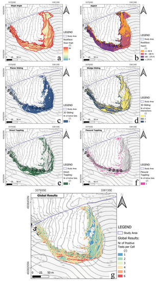
Figure 10.
From top to bottom: (a) slope and (b) aspect of the studied rock mass; the outputs of the AMTT algorithm, defining where each type of movement is possible: (c) planar sliding, (d) wedge sliding, (e) direct toppling and (f) flexural toppling; (g) how many sets or intersections are active.
It is clear how the most common type of movement is Wedge Sliding (or 3D Sliding), which corroborates what was derived from the simple observation of the orientation of the three main discontinuity sets. Planar Sliding (or 2D Sliding) is also very diffused, controlled, as previously said, by K1 and K2 on the east-facing and south-facing sides, respectively. Less common but still important is Direct Toppling, while Flexural Toppling appears as the least significant type of movement. The combined results shown in the last image of Figure 10 make clear that the most active side of the rock mass is the south-facing one, where locations with up to six positive tests can be found.
Each cell of the AMTT output grid files where at least one of the kinematic tests turns out positive is a possible source location for rockfall and as such has been considered in the 3D simulations. The values of the rock density, the block type (i.e., prismatic) and the three main dimensions of the reference block have to be associated with each source cell for Rockyfor3D to work. For the rock density, a standard of 2.700 kg/m3 was selected, as it represents a good approximation of the density of the quartzites identified on site. Regarding the block size, for each shape, a set of three values was extracted from the spacing distributions: the condition was that the product of the three spacings had to be equal to 6.5 m3 and the ratios between the lengths respected the distinctions imposed to identify each of the four block shapes [25]. Table 5 summarizes these data. All blocks were assumed to be prismatic, as testified by the ones visible in situ and the reciprocal orientation of the three joint sets identified in the rock mass.
Table 5.
Value of the length of the three sides of the prismatic block for each of the block shapes.
Lastly, a DSM of the area is required: for the scale of the study area, the DSM freely provided by the Piemonte Region [46] was deemed enough. This DSM has a cell size of 5 × 5 m and a vertical accuracy of 0.5–0.6 m in non-urban areas.
Four different simulations were performed to evaluate the contribution of every shape; each of these simulations accounted for 1.000 blocks falling from each source cell. Each of the outputs of the four simulations has been combined to obtain a global result. This is visible in Figure 11 for the Reach Probability map. Figure 12, Figure 13, Figure 14 and Figure 15 show the other output maps: the Number of Passages per cell, which highlights the preferential runout paths, the Number of Depositions per cell, which visualizes depositional areas, the Total Kinetic Energy and the Bounces Height. From the Number of Passages and Number of Depositions maps, it is clear that most of the blocks that fell from the studied rock mass are either stopped by the reliefs just upslope with respect to the buildings of Grangia Cruset or are channeled towards the wide slope to its east and then stop in the flat area next to the road. The distribution of the simulated depositions also maps quite precisely the real deposits, with large blocks and boulders mapped in the study area. Clearly, it is the east-facing side of the rock mass that is more likely to produce blocks that are able to reach the lowermost portion of the study area and the buildings located there. On the one hand, this is good: the exposed buildings are protected from the most cinematically active portion of the rock mass by the natural topographical features of the area. On the other hand, though, rockfall originating on the east-facing side of the rock mass has a significantly longer runout along a steep slope. This means that those blocks have a higher probability of reaching higher energy levels. This is corroborated by the Total Kinetic Energy map, where high energy values are mostly located in the lower half of the eastern slope, and by the Reach Probability map, where we see values above 1% in the lower sector of the study area only on the eastern slope.
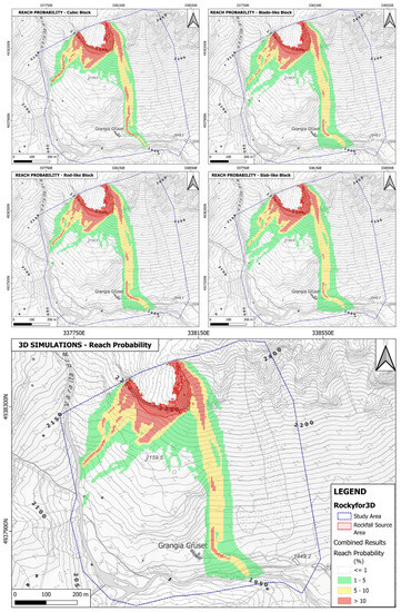
Figure 11.
The Reach Probability maps for each of the four shape types (cubic, blade, rod and slab) and the combined Global Map.
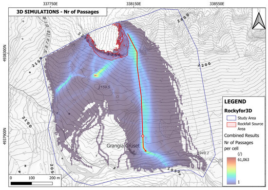
Figure 12.
The global map describing the number of blocks passing through each cell; the red arrow indicates the main runout path used to identify the topographic profile for the following 2D numerical simulations; the red and white dots correspond to the selected location to extract the DSCs from the 2D simulations.
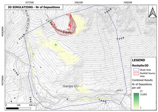
Figure 13.
The global map describing the number of blocks stopping in each cell.
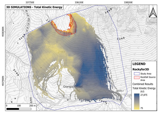
Figure 14.
The global map describing the Total Kinetic Energy in each cell.
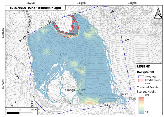
Figure 15.
The global map describing the Bounces Height in each cell.
As visible in Figure 12, on the Number of Passages map, the preferential runout path was selected. It is important to notice how that map shows actually more than one preferential path, both in the eastern portion of the slope and in the western portion. We focused only on the eastern one due to the fact that the other paths led only towards the depositional area above Grangia Cruset, without interacting with the existing buildings, while the eastern path ends up quite or very close to them. Moreover, as stated before, this portion of the slope shows higher energy values. Following the red arrow in Figure 12, a topographic profile was extracted from the 5 × 5 m DSM and plugged in Rocfall2 alongside the IBSD of the rock mass. A set of one thousand simulations was performed, and the data regarding the bounces height and total kinetic energy was extracted. To do so, a position of interest had to be selected, corresponding to the red and white dots in Figure 12. From the same slope model employed for the 3D simulations (in Figure 6), the restitution coefficients of the topographic profile were selected.
4.3. Phase 3
The Global Reach Probability map (Figure 11) allows the observer to appreciate two key features. First of all, the high (in red) and intermediate (in yellow) probability areas are very concentrated along the preferential run-out paths visible in Figure 12: this means that rockfall events show a significant tendency to follow those paths, only straying from them in very rare instances, a fact that is actually supported by the evidence of past recorded events and the arrangement of actual blocks found along the slope. Second, it appears that the buildings at Grangia Cruset are just outside a low-probability-of-being-reached area (in green in Figure 11). This suggests that what happened on 22 July 2017, when the 6 m3 block reached the buildings and than proceeded downslope towards the river, was a very unlikely event to occur, at least according to our models. It is important to know that the area outside the low-probability sectors in Figure 11 does have a very low Reach Probability, numbering between 0 and 1%.
From the output of the 2D numerical simulations, the two DSCs for the Total Kinetic Energy and for the Bounces Height were drawn (Figure 16 and Figure 17). As stated in Section 2.3, a DSC is intended to be used in different ways: to directly choose the energy level of the protection works and to quantify the protection provided by them or as direct input in advanced design methods. For instance, assuming that an acceptable level of residual probability of being exceeded cannot be higher than 10%, applying the first approach would mean designing a defensive structure capable of withstanding 27,000 kJ upon impact. In terms of the height of the structure, the same acceptable level of residual probability of being exceeded on the Bounces Height DSC would point towards a protection work at least 2.5 m high. Both values are visible in the respective figures. Considering the actual number and value of the exposed buildings, such a protection level would require the construction of an embankment, a solution far too costly and, therefore, unrealistic. For these reasons, other more economically viable solutions could be explored.
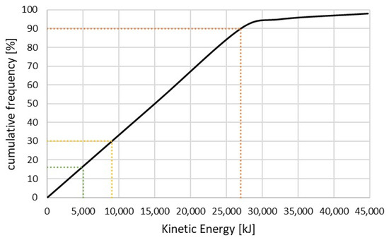
Figure 16.
DSC for the Total Kinetic Energy: to achieve a protection efficiency of 90%, a protection work has to be able to withstand energies of at least 27,000 kJ (in red). A 5000 kJ (in green) or 10,000 kJ (in orange) flexible barrier would not be particularly efficient.
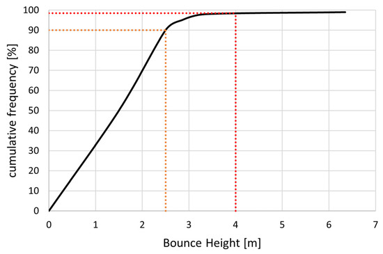
Figure 17.
DSC for the Bounces Height: to achieve a protection efficiency of 90%, a protection work has to be at least 2.5 m high (in orange). A 4 m high rockfall flexible barrier (in red) would be even more efficient.
To demonstrate how a DSC can be used to verify the efficiency of a protection work, the use of a standard flexible rockfall barrier has been considered. In fact, such a protection work was actually installed after the last recorded rockfall, just east with respect to the buildings of Grangia Cruset. The Service Energy Level (SEL) of that barrier is not known. In Figure 16, the effectiveness in terms of the probability of not being exceeded of the SEL of two barrier kits is presented, while in Figure 17, the effectiveness of a barrier 4 m high is shown. The service energy level of the two barriers corresponds to 10,000 and 5000 kJ: these are, respectively, the maximum energy level of commercial flexible barriers and 50% of it. Here, these two kits are presented purely as an example, but the values were selected because of the exceedingly high energy requirements, also portrayed in Figure 16. In fact, as can be seen, in terms of energy, none of the two selected kits provide significant levels of protection: the probability of not being exceeded is 18% for the 5000 kJ kit and 30% for the 10,000 kJ one, which is undoubtedly in favor of the second one but not even closely satisfactory. The chosen height of 4 m is instead exceedingly effective.
The last design approach made possible with DSCs is not discussed here: the actual implementation of these curves in terms of input values—for example, for a Reliability-Based Design method—is theoretically possible but has not yet been effectively tested.
It is important to clarify that the solutions explored here are intended only as an example: in reality, given the logistical issues of the study area, the position and the value of the exposed buildings, there would be no economically feasible solution to the problem. In fact, the existing flexible barriers were put in place to protect only from small or very small blocks, with volumes lower than 1.5 m3 at best.
5. Conclusions
The development of advanced terrestrial or aerial measurement techniques aimed at the definition of the geometrical features of rock slopes becomes a real asset for land management and landslide risk mitigation if supported by appropriate data analysis tools, extracting and quantifying the data necessary for the design phase. This work presents the developments of algorithms, codes and, particularly, procedures carried out by the authors and aimed at quantifying different ruling parameters in rockfall phenomena such as: the volume and shape of potentially unstable blocks, possible areas of detachment and types of kinematics. The results are then used as input data in the analysis of the trajectories based on bot 3D and 2D numerical simulations, performed with commercial codes: this allows for parametric analyses to be carried out in order to quantify, in statistical terms, the various parameters considered. The application of the methodology to a real case has shown its potential in terms of the statistical distribution of the main quantities, such as the kinetic energies of the blocks and the heights of bounces along the trajectories, which are necessary for the choice and sizing of the protection structures. The key aspect of this approach is its complete reliance on quantitative descriptions of the quantities involved, independent of the actual methodology used in the end, during the design phase.
The main innovative aspects of the methodology presented in this paper are summarized as follows:
- The use of an IBSD curve to describe in probabilistic terms the full spectrum of block sizes geometrically possible in a rock mass, compared to the deterministic and empirically based choice of a single value;
- The use of a shape distribution to describe the relative abundance of shapes geometrically possible in a rock mass and its implementation in the numerical simulations, compared to the deterministic choice of one reference shape;
- The use of probabilistic output descriptors for key design parameters, describing the full spectrum of possibilities. This allows for a quantitative choice of those parameters, for the evaluation of the efficiency of selected protection works and even for the implementation of more sophisticated non-standard design techniques.
This work is preparatory to a holistic development of the design of risk mitigation systems for mountain basins where the complexity of the phenomena requires a parametric analysis of the factors involved to achieve an optimal choice of the type of works, their location and their size, also accounting for their efficiency in terms of residual risk. The method is indeed based upon existing techniques and processes of proven value and reliability but is the first proposing combining and streamlining them into a complete workflow.
Author Contributions
Conceptualization, B.T. and G.U.; methodology, B.T. and G.U.; software, B.T. and G.U.; validation, G.U., A.M.F. and B.T.; formal analysis, G.U. and B.T.; investigation, G.U. and B.T.; resources, A.M.F. and G.U.; data curation, G.U. and B.T.; writing—original draft preparation, B.T. and G.U.; writing—review and editing, A.M.F., G.U. and B.T.; visualization, B.T. and G.U.; supervision, G.U. and A.M.F.; project administration, G.U. and A.M.F. All authors have read and agreed to the published version of the manuscript.
Funding
This research received no external funding.
Data Availability Statement
The data presented in this study are available on request from the corresponding author. The data are not yet publicly available due to ongoing research activities.
Conflicts of Interest
The authors declare no conflict of interest.
References
- Bemis, S.P.; Micklethwaite, S.; Turner, D.; James, M.R.; Akciz, S.; Thiele, S.T.; Bangash, H.A. Ground-based and UAV-Based photogrammetry: A multi-scale, high-resolution mapping tool for structural geology and paleoseismology. J. Struct. Geol. 2014, 69, 163–178. [Google Scholar] [CrossRef]
- Kong, D.; Saroglou, C.; Wu, F.; Sha, P.; Li, B. Development and application of UAV-SfM photogrammetry for quantitative characterization of rock mass discontinuities. Int. J. Rock Mech. Min. Sci. 2021, 141, 104729. [Google Scholar] [CrossRef]
- Herrero, M.J.; Pérez-Fortes, A.P.; Escavy, J.I.; Insua-Arévalo, J.M.; De la Horra, R.; López-Acevedo, F.; Trigos, L. 3D model generated from UAV photogrammetry and semi-automated rock mass characterization. Comput. Geosci. 2022, 163, 105121. [Google Scholar] [CrossRef]
- Mineo, S.; Caliò, D.; Pappalardo, G. UAV-Based Photogrammetry and Infrared Thermography Applied to Rock Mass Survey for Geomechanical Purposes. Remote Sens. 2022, 14, 473. [Google Scholar] [CrossRef]
- Riquelme, A.J.; Abellan, A.; Tomás, R. Discontinuity spacing analysis in rock masses using 3D point clouds. Eng. Geol. 2015, 195, 185–195. [Google Scholar] [CrossRef]
- Riquelme, A.; Tomás, R.; Cano, M.; Pastor, J.L.; Abellán, A. Automatic Mapping of Discontinuity Persistence on Rock Masses Using 3D Point Clouds. Rock Mech. Rock Eng. 2018, 51, 3005–3028. [Google Scholar] [CrossRef]
- Umili, G. Methods for sampling discontinuity traces on rock mass 3D models: State of the art. IOP Conf. Ser. Earth Environ. Sci. 2021, 833, 012050. [Google Scholar] [CrossRef]
- Chen, S.; Walske, M.L.; Davies, I.J. Rapid mapping and analysing rock mass discontinuities with 3D terrestrial laser scanning in the underground excavation. Int. J. Rock Mech. Min. Sci. 2018, 110, 28–35. [Google Scholar] [CrossRef]
- Saricam, I.T.; Ozturk, H. Joint roughness profiling using photogrammetry. Appl. Geomat. 2022, 14, 573–587. [Google Scholar] [CrossRef]
- Chen, K.; Jiang, Q. A non-contact measurement method for rock mass discontinuity orientations by smartphone. J. Rock Mech. Geotech. Eng. 2022. [Google Scholar] [CrossRef]
- Migliazza, M.; Carriero, M.T.; Lingua, A.; Pontoglio, E.; Scavia, C. Rock Mass Characterization by UAV and Close-Range Photogrammetry: A Multiscale Approach Applied along the Vallone dell’Elva Road (Italy). Geosciences 2021, 11, 436. [Google Scholar] [CrossRef]
- Caliò, D.; Mineo, S.; Pappalardo, G. Digital Rock Mass Analysis for the Evaluation of Rockfall Magnitude at Poorly Accessible Cliffs. Remote Sens. 2023, 15, 1515. [Google Scholar] [CrossRef]
- Mineo, S.; Pappalardo, G.; Onorato, S. Geomechanical Characterization of a Rock Cliff Hosting a Cultural Heritage through Ground and UAV Rock Mass Surveys for Its Sustainable Fruition. Sustainability 2021, 13, 924. [Google Scholar] [CrossRef]
- Giordan, D.; Manconi, A.; Tannant, D.D.; Allasia, P. UAV: Low-cost remote sensing for high-resolution investigation of landslides. In Proceedings of the International Geosciences and Remote Sensing Symposium (IGARSS), Milan, Italy, 26–31 July 2015; pp. 5344–5347. [Google Scholar] [CrossRef]
- Rodriguez, J.; Macciotta, R.; Hendry, M.T.; Roustaei, M.; Gräpel, C.; Skirrow, R. UAVs for monitoring, investigation, and mitigation design of a rock slope with multiple failure mechanisms—A case study. Landslides 2020, 17, 2027–2040. [Google Scholar] [CrossRef]
- Abbruzzese, J.M.; Labiouse, V. New Cadanav Methodology for Rock Fall Hazard Zoning Based on 3D Trajectory Modelling. Geosciences 2020, 10, 434. [Google Scholar] [CrossRef]
- Wang, W.; Zhao, W.; Chai, B.; Du, J.; Tang, L.; Yi, X. Discontinuity interpretation and identification of potential rockfalls for high-steep slopes based on UAV nap-of-the-object photogrammetry. Comput. Geosci. 2022, 166, 105191. [Google Scholar] [CrossRef]
- Umili, G.; Taboni, B.; Ferrero, A.M. Influence of uncertainties: A focus on block volume and shape assessment for rockfall analysis. J. Rock Mech. Geotech. Eng. 2023, 15, 2250–2263. [Google Scholar] [CrossRef]
- Umili, G.; Bonetto, S.M.R.; Mosca, P.; Vagnon, F.; Ferrero, A.M. In Situ Block Size Distribution Aimed at the Choice of the Design Block for Rockfall Barriers Design: A Case Study along Gardesana Road. Geosciences 2020, 10, 223. [Google Scholar] [CrossRef]
- Lu, P.; Latham, J.-P. Developments in the Assessment of In-situ Block Size Distributions of Rock Masses. Rock Mech. Rock Eng. 1999, 32, 29–49. [Google Scholar] [CrossRef]
- Wang, H.; Latham, J.-P.; Poole, A.B. In situ block size assessment from discontinuity spacing data. Int. J. Rock Mech. Min. Sci. Geomech. Abstr. 1993, 30, A106. [Google Scholar] [CrossRef]
- Wang, H.; Latham, J.-P.; Poole, A.B. Predictions of block size distribution for quarrying. Q. J. Eng. Geol. 1991, 24, 91–99. [Google Scholar] [CrossRef]
- Leine, R.I.; Capobianco, G.; Bartelt, P.; Christen, M.; Caviezel, A. Stability of rigid body motion through an extended intermediate axis theorem: Application to rockfall simulation. Multibody Syst. Dyn. 2021, 52, 431–455. [Google Scholar] [CrossRef]
- Lu, G.; Ringenbach, A.; Caviezel, A.; Sanchez, M.; Christen, M.; Bartelt, P. Mitigation effects of trees on rockfall hazards: Does rock shape matter? Landslides 2021, 18, 59–77. [Google Scholar] [CrossRef]
- Palmstrom, A. Measurement and characterization of rock mass jointing. In In-Situ Characterization of Rocks; Sharma, V.M., Saxena, K.R., Eds.; A. A. Balkema Publishers: Rotterdam, The Netherlands, 2001; pp. 49–97. [Google Scholar]
- Kalenchuk, K.S.; Diederichs, M.S.; McKinnon, S. Characterizing block geometry in jointed rockmasses. Int. J. Rock Mech. Min. Sci. 2006, 43, 1212–1225. [Google Scholar] [CrossRef]
- Dorren, L.K.A. Rockyfor3D, Revealed—Transparent Description of the Complete 3D Rockfall Model; ecorisQ paper (www.ecorisq.org); Int. ecorisQ Association: Geneva, Switzerland, 2016; p. 33. [Google Scholar]
- Noël, F.; Cloutier, C.; Jaboyedoff, M.; Locat, J. Impact-Detection Algorithm That Uses Point Clouds as Topographic Inputs for 3D Rockfall Simulations. Geosciences 2021, 11, 188. [Google Scholar] [CrossRef]
- Leine, R.I.; Schweizer, A.; Christen, M.; Glover, J.; Bartelt, P.; Gerber, W. Simulation of rockfall trajectories with consideration of rock shape. Multibody Syst. Dyn. 2014, 32, 241–271. [Google Scholar] [CrossRef]
- Sistema Informativo Fenomeni Franosi Piemonte (SIFRAP). Available online: https://webgis.arpa.piemonte.it/geodissesto/sifrap/iilivelli.php (accessed on 24 May 2023).
- Bourrier, F.; Toe, D.; Garcia, B.; Baroth, J.; Lambert, S. Experimental investigations on complex block propagation for the assessment of propagation models quality. Landslides 2021, 18, 639–654. [Google Scholar] [CrossRef]
- Vöge, M.; Lato, M.J.; Diederichs, M.S. Automated rockmass discontinuity mapping from 3-dimensional surface data. Eng. Geol. 2013, 164, 155–162. [Google Scholar] [CrossRef]
- Riquelme, A.J.; Abellán, A.; Tomás, R.; Jaboyedoff, M. A new approach for semi-automatic rock mass joints recognition from 3D point clouds. Comput. Geosci. 2014, 68, 38–52. [Google Scholar] [CrossRef]
- Gomes, R.K.; De Oliveira, L.P.L.; Gonzaga, L.; Tognoli, F.M.W.; Veronez, M.R.; De Souza, M.K. An algorithm for au-tomatic detection and orientation estimation of planar structures in LiDAR-scanned outcrops. Comput. Geosci. 2016, 90, 170–178. [Google Scholar] [CrossRef]
- Buyer, A.; Aichinger, S.; Schubert, W. Applying photogrammetry and semi-automated joint mapping for rock mass characterization. Eng. Geol. 2020, 264, 105332. [Google Scholar] [CrossRef]
- Kong, D.; Wu, F.; Saroglou, C. Automatic identification and characterization of discontinuities in rock masses from 3D point clouds. Eng. Geol. 2020, 265, 105442. [Google Scholar] [CrossRef]
- Taboni, B.; Tagliaferri, I.D.; Umili, G. A Tool for Performing Automatic Kinematic Analysis on Rock Outcrops. Geosciences 2022, 12, 435. [Google Scholar] [CrossRef]
- Palmstrøm, A. Characterizing rock masses by the RMi for use in practical rock engineering. Tunn. Undergr. Space Technol. 1996, 11, 175–188. [Google Scholar] [CrossRef]
- Widmann, R. International Society for Rock Mechanics (ISRM) commission on standardization of laboratory and field tests. Suggested methods for the quantitative description of discontinuities in rock masses. Int. J. Rock Mech. Min. Sci. 1978, 15, 319–368. [Google Scholar]
- Markland, J.T. A usefull technique for estimating the stability of rock slopes when the rigid wedge slide type of failure is expected. In Interdepartment Rock Mechanics Project; Imperial College of Science and Technology: London, UK, 1972. [Google Scholar]
- Rocscience. Rocfall2. Available online: https://www.rocscience.com/software/rocfall (accessed on 5 March 2023).
- Low, B.K. Reliability-Based Design in Soil and Rock Engineering: Enhancing Partial Facctor Design Approaches, 1st ed.; CRC Press: Boca Raton, FL, USA, 2021. [Google Scholar] [CrossRef]
- Low, B. Reliability analysis of rock slopes involving correlated nonnormals. Int. J. Rock Mech. Min. Sci. 2007, 44, 922–935. [Google Scholar] [CrossRef]
- Low, B.K.; Tang, W.H.; Low, M.B.K.; Member, A.; Fellow, A. Efficient Reliability Evaluation Using Spreadsheet. J. Eng. Mech. 1997, 123, 749–752. [Google Scholar] [CrossRef]
- Ferrero, A.M.; Forlani, G.; Roncella, R.; Voyat, H.I. Advanced Geostructural Survey Methods Applied to Rock Mass Characterization. Rock Mech. Rock Eng. 2009, 42, 631–665. [Google Scholar] [CrossRef]
- Regione Piemonte, Digital Terrain Model (DTM). Available online: https://www.geoportale.piemonte.it/geonetwork/srv/ita/catalog.search#/metadata/r_piemon:224de2ac-023e-441c-9ae0-ea493b217a8e (accessed on 3 March 2023).
Disclaimer/Publisher’s Note: The statements, opinions and data contained in all publications are solely those of the individual author(s) and contributor(s) and not of MDPI and/or the editor(s). MDPI and/or the editor(s) disclaim responsibility for any injury to people or property resulting from any ideas, methods, instructions or products referred to in the content. |
© 2023 by the authors. Licensee MDPI, Basel, Switzerland. This article is an open access article distributed under the terms and conditions of the Creative Commons Attribution (CC BY) license (https://creativecommons.org/licenses/by/4.0/).