


Applying High-Resolution Satellite and UAS Imagery for Detecting Coldwater Inputs in Temperate Streams of the Iowa Driftless Region


Abstract
:1. Introduction
2. Materials and Methods
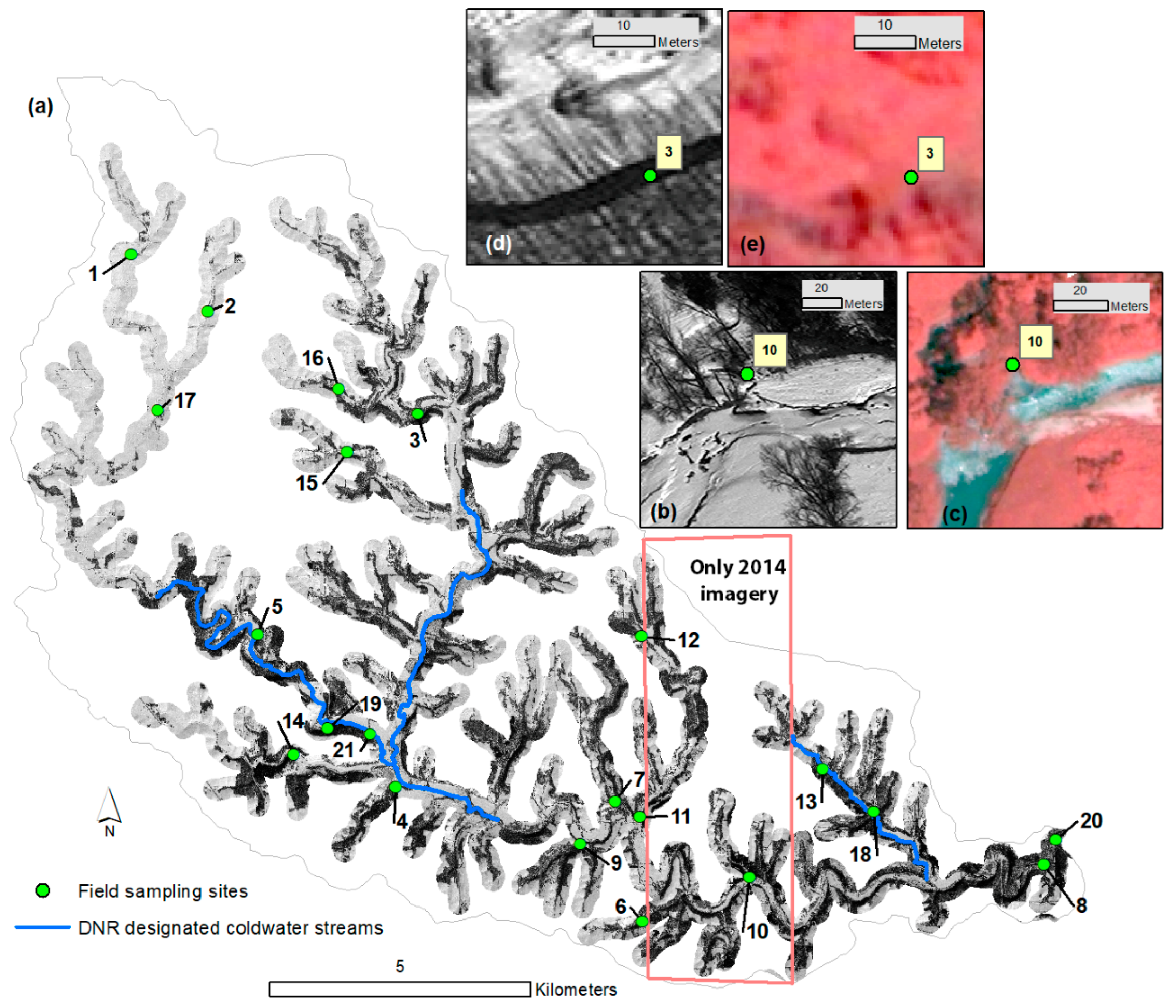
2.1. Study Area
2.2. Water Temperature Assessments
2.3. Fish Community Assessments
2.4. Uncrewed Aerial System (UAS) Survey
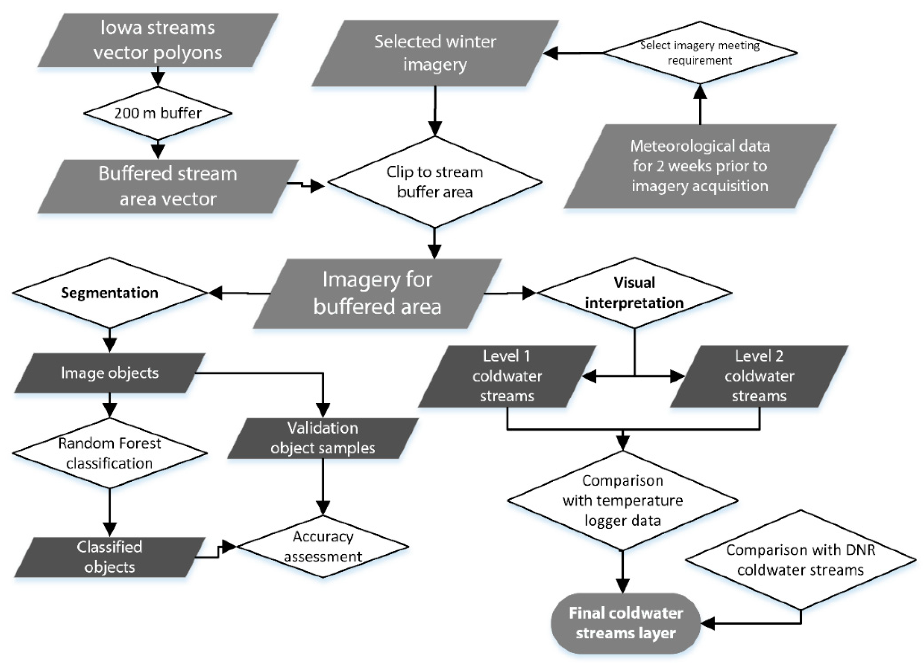
2.5. Image Selection, Pre-Processing, and Analysis
3. Results
3.1. Water Temperature Monitoring
3.2. Fish Communities
3.3. UAS Imagery Assessment
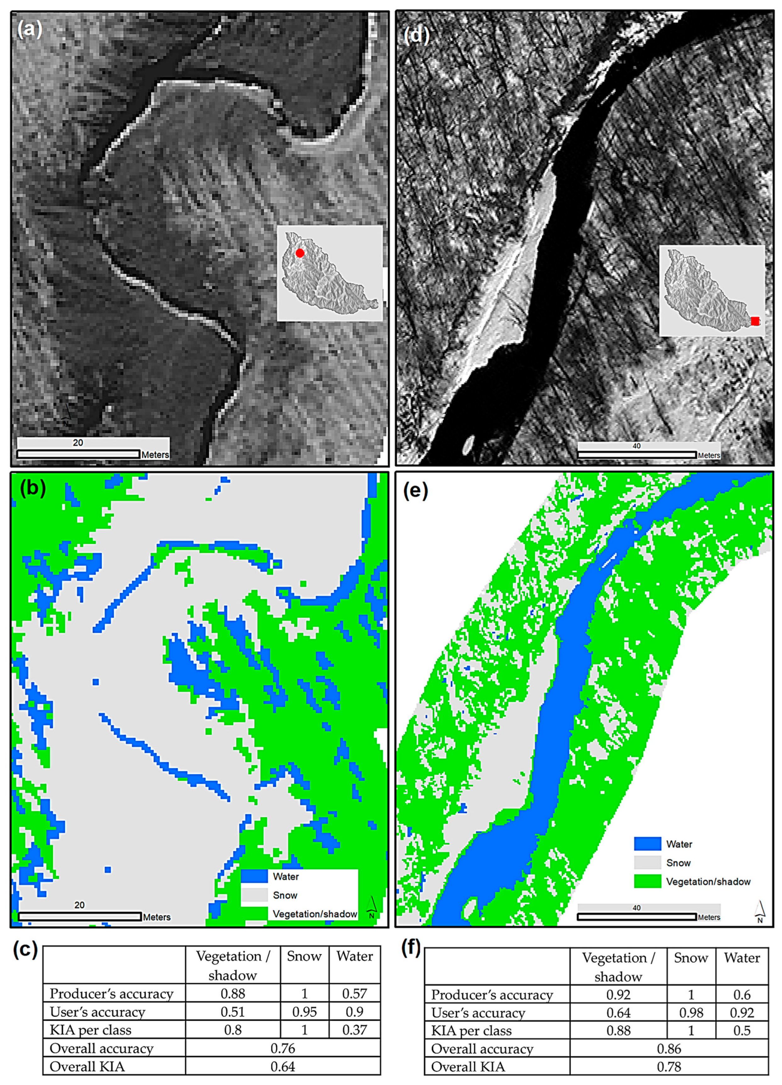
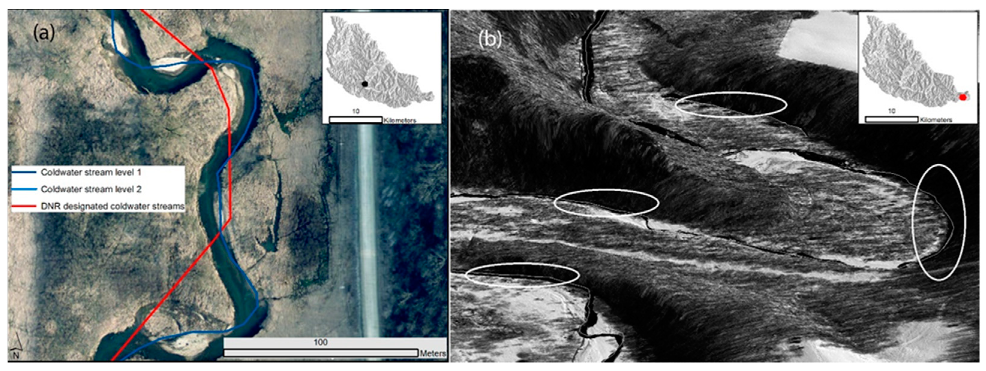
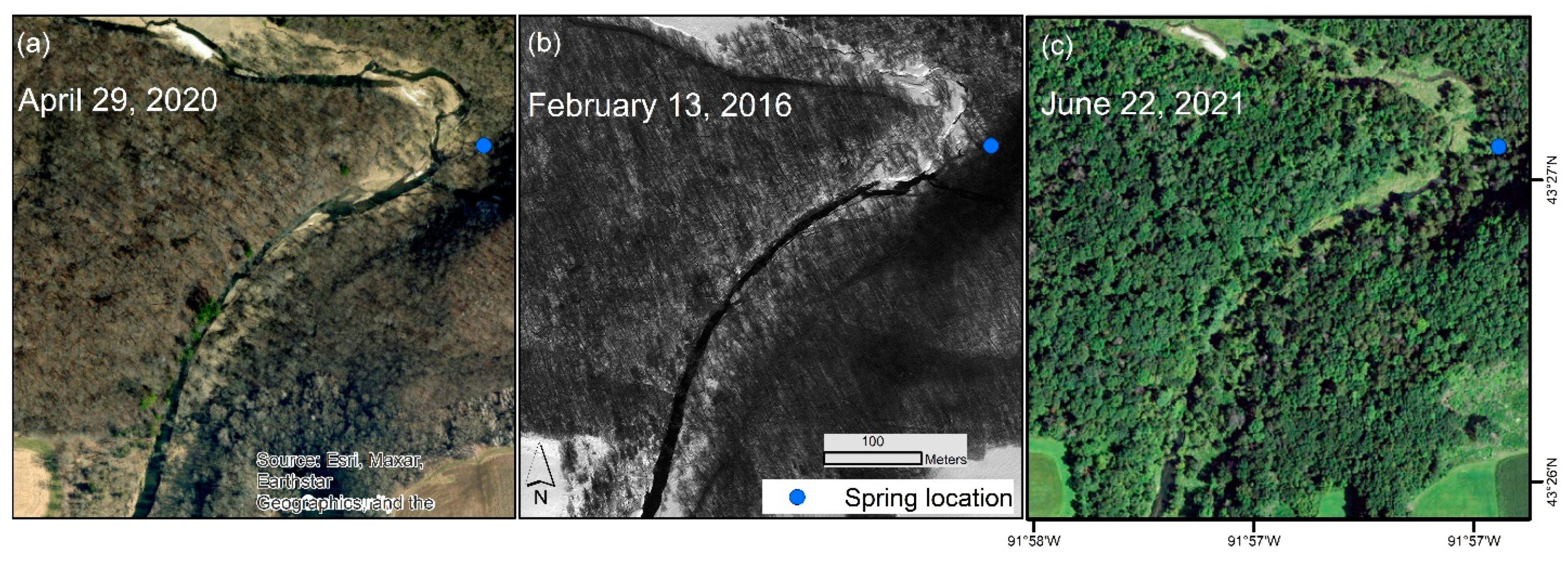
3.4. VHR Winter Imagery Assessment
4. Discussion
5. Conclusions
Supplementary Materials
Author Contributions
Funding
Data Availability Statement
Acknowledgments
Conflicts of Interest
References
- Allan, J.D.; Castillo, M.M.; Capps, K.A. Stream Ecology: Structure and Function of Running Waters; Springer Nature: Berlin, Germany, 2020. [Google Scholar]
- Muhlfeld, C.C. Cold-water species need warm water too. Nat. Clim. Change 2021, 11, 297–299. [Google Scholar] [CrossRef]
- Linnansaari, T.; Cunjak, R.A. Patterns in apparent survival of Atlantic salmon (Salmo salar) parr in relation to variable ice conditions throughout winter. Can. J. Fish. Aquat. Sci. 2010, 67, 1744–1754. [Google Scholar] [CrossRef]
- Kurylyk, B.; MacQuarrie, K.; Caissie, D.; McKenzie, J. Shallow groundwater thermal sensitivity to climate change and land cover disturbances: Derivation of analytical expressions and implications for stream temperature projections. Hydrol. Earth Syst. Sci. Discuss. 2014, 11, 12573–12626. [Google Scholar] [CrossRef]
- Lyons, J.; Zorn, T.; Stewart, J.; Seelbach, P.; Wehrly, K.; Wang, L. Defining and characterizing coolwater streams and their fish assemblages in Michigan and Wisconsin, USA. N. Am. J. Fish. Manag. 2009, 29, 1130–1151. [Google Scholar] [CrossRef]
- Gresswell, R.E.; Vondracek, B. Coldwater Streams. In Inland Fisheries Management in North America, 3rd ed.; American Fisheries Society: Bethsda, MD, USA, 2010; pp. 587–618. [Google Scholar]
- McCullough, D.A.; Bartholow, J.M.; Jager, H.I.; Beschta, R.L.; Cheslak, E.F.; Deas, M.L.; Ebersole, J.L.; Foott, J.S.; Johnson, S.L.; Marine, K.R. Research in thermal biology: Burning questions for coldwater stream fishes. Rev. Fish. Sci. 2009, 17, 90–115. [Google Scholar] [CrossRef]
- Isaak, D.J.; Young, M.K.; Nagel, D.E.; Horan, D.L.; Groce, M.C. The cold-water climate shield: Delineating refugia for preserving salmonid fishes through the 21st century. Glob. Change Biol. 2015, 21, 2540–2553. [Google Scholar] [CrossRef]
- Wang, L.; Kanehl, P. Influences of watershed urbanization and instream habitat on macroinvertebrates in cold water streams 1. JAWRA J. Am. Water Resour. Assoc. 2003, 39, 1181–1196. [Google Scholar] [CrossRef]
- Barquín, J.; Scarsbrook, M. Management and conservation strategies for coldwater springs. Aquat. Conserv. Mar. Freshw. Ecosyst. 2008, 18, 580–591. [Google Scholar] [CrossRef]
- Santiago, J.M.; Muñoz-Mas, R.; Solana-Gutiérrez, J.; Garcia de Jalon, D.; Alonso, C.; Martínez-Capel, F.; Pórtoles, J.; Monjo, R.; Ribalaygua, J. Waning habitats due to climate change: The effects of changes in streamflow and temperature at the rear edge of the distribution of a cold-water fish. Hydrol. Earth Syst. Sci. 2017, 21, 4073–4101. [Google Scholar] [CrossRef]
- Hauer, R.; Lamberti, G.A. Methods in Stream Ecology; Academic Press: Cambridge, MA, USA, 2011. [Google Scholar]
- Chapin, T.P.; Todd, A.S.; Zeigler, M.P. Robust, low-cost data loggers for stream temperature, flow intermittency, and relative conductivity monitoring. Water Resour. Res. 2014, 50, 6542–6548. [Google Scholar] [CrossRef]
- Nelson, K.C.; Palmer, M.A. Stream temperature surges under urbanization and climate change: Data, models, and responses 1. JAWRA J. Am. Water Resour. Assoc. 2007, 43, 440–452. [Google Scholar] [CrossRef]
- Webb, B.W.; Hannah, D.M.; Moore, R.D.; Brown, L.E.; Nobilis, F. Recent advances in stream and river temperature research. Hydrol. Process. Int. J. 2008, 22, 902–918. [Google Scholar] [CrossRef]
- O’Sullivan, A.M.; Linnansaari, T.; Curry, R.A. Ice cover exists: A quick method to delineate groundwater inputs in running waters for cold and temperate regions. Hydrol. Process. 2019, 33, 3297–3309. [Google Scholar] [CrossRef]
- Sass, G.; Creed, I.; Riddell, J.; Bayley, S. Regional-scale mapping of groundwater discharge zones using thermal satellite imagery. Hydrol. Process. 2014, 28, 5662–5673. [Google Scholar] [CrossRef]
- Vanderhoof, M.K.; Burt, C. Applying high-resolution imagery to evaluate restoration-induced changes in stream condition, Missouri River Headwaters Basin, Montana. Remote Sens. 2018, 10, 913. [Google Scholar] [CrossRef]
- Dugdale, S.J. A practitioner’s guide to thermal infrared remote sensing of rivers and streams: Recent advances, precautions and considerations. Wiley Interdiscip. Rev. Water 2016, 3, 251–268. [Google Scholar] [CrossRef]
- Murphy Jr, R.D.; Hagan, J.A.; Harris, B.P.; Sethi, S.A.; Smeltz, T.S.; Restrepo, F. Can Landsat Thermal Imagery and Environmental Data Accurately Estimate Water Temperatures in Small Streams? J. Fish Wildl. Manag. 2021, 12, 12–26. [Google Scholar] [CrossRef]
- Martí-Cardona, B.; Prats, J.; Niclòs, R. Enhancing the retrieval of stream surface temperature from Landsat data. Remote Sens. Environ. 2019, 224, 182–191. [Google Scholar] [CrossRef]
- Handcock, R.N.; Torgersen, C.E.; Cherkauer, K.A.; Gillespie, A.R.; Tockner, K.; Faux, R.N.; Tan, J.; Carbonneau, P. Thermal infrared remote sensing of water temperature in riverine landscapes. Fluv. Remote Sens. Sci. Manag. 2012, 1, 85–113. [Google Scholar]
- Huang, C.; Chen, Y.; Zhang, S.; Wu, J. Detecting, extracting, and monitoring surface water from space using optical sensors: A review. Rev. Geophys. 2018, 56, 333–360. [Google Scholar] [CrossRef]
- Dugdale, S.J.; Kelleher, C.A.; Malcolm, I.A.; Caldwell, S.; Hannah, D.M. Assessing the potential of drone-based thermal infrared imagery for quantifying river temperature heterogeneity. Hydrol. Process. 2019, 33, 1152–1163. [Google Scholar] [CrossRef]
- Caldwell, S.; Kelleher, C.; Baker, E.; Lautz, L.K. Relative information from thermal infrared imagery via unoccupied aerial vehicle informs simulations and spatially-distributed assessments of stream temperature. Sci. Total Environ. 2019, 661, 364–374. [Google Scholar] [CrossRef] [PubMed]
- Casas-Mulet, R.; Pander, J.; Ryu, D.; Stewardson, M.J.; Geist, J. Unmanned Aerial Vehicle (UAV)-Based Thermal Infra-Red (TIR) and Optical Imagery Reveals Multi-Spatial Scale Controls of Cold-Water Areas Over a Groundwater-Dominated Riverscape. Front. Environ. Sci. 2020, 8, 64. [Google Scholar] [CrossRef]
- Briggs, M.A.; Dawson, C.B.; Holmquist-Johnson, C.L.; Williams, K.H.; Lane, J.W. Efficient hydrogeological characterization of remote stream corridors using drones. Hydrol. Process. 2018, 33, 316–319. [Google Scholar] [CrossRef]
- Morgan, A.M.; O’Sullivan, A.M. Cooler, bigger; warmer, smaller: Fine-scale thermal heterogeneity maps age class and species distribution in behaviourally thermoregulating salmonids. River Res. Appl. 2023, 39, 163–176. [Google Scholar] [CrossRef]
- Kuhn, J.; Casas-Mulet, R.; Pander, J.; Geist, J. Assessing stream thermal heterogeneity and cold-water patches from UAV-based imagery: A matter of classification methods and metrics. Remote Sens. 2021, 13, 1379. [Google Scholar] [CrossRef]
- Marcus, W.A.; Fonstad, M.A. Optical remote mapping of rivers at sub-meter resolutions and watershed extents. Earth Surf. Process. Landf. J. Br. Geomorphol. Res. Group 2008, 33, 4–24. [Google Scholar] [CrossRef]
- Dufour, S.; Bernez, I.; Betbeder, J.; Corgne, S.; Hubert-Moy, L.; Nabucet, J.; Rapinel, S.; Sawtschuk, J.; Trollé, C. Monitoring restored riparian vegetation: How can recent developments in remote sensing sciences help? Knowl. Manag. Aquat. Ecosyst. 2013, 410, 10. [Google Scholar] [CrossRef]
- Espel, D.; Courty, S.; Auda, Y.; Sheeren, D.; Elger, A. Submerged macrophyte assessment in rivers: An automatic mapping method using Pléiades imagery. Water Res. 2020, 186, 116353. [Google Scholar] [CrossRef]
- Ade, C.; Khanna, S.; Lay, M.; Ustin, S.L.; Hestir, E.L. Genus-level mapping of invasive floating aquatic vegetation using Sentinel-2 satellite remote sensing. Remote Sens. 2022, 14, 3013. [Google Scholar] [CrossRef]
- Chaudhuri, G.; Mishra, N.B. Detection of Aquatic Invasive Plants in Wetlands of the Upper Mississippi River from UAV Imagery Using Transfer Learning. Remote Sens. 2023, 15, 734. [Google Scholar] [CrossRef]
- Sagan, V.; Peterson, K.T.; Maimaitijiang, M.; Sidike, P.; Sloan, J.; Greeling, B.A.; Maalouf, S.; Adams, C. Monitoring inland water quality using remote sensing: Potential and limitations of spectral indices, bio-optical simulations, machine learning, and cloud computing. Earth-Sci. Rev. 2020, 205, 103187. [Google Scholar] [CrossRef]
- Yigit Avdan, Z.; Kaplan, G.; Goncu, S.; Avdan, U. Monitoring the water quality of small water bodies using high-resolution remote sensing data. ISPRS Int. J. Geo-Inf. 2019, 8, 553. [Google Scholar] [CrossRef]
- He, B.; Oki, K.; Wang, Y.; Oki, T.; Yamashiki, Y.; Takara, K.; Miura, S.; Imai, A.; Komatsu, K.; Kawasaki, N. Analysis of stream water quality and estimation of nutrient load with the aid of Quick Bird remote sensing imagery. Hydrol. Sci. J. 2012, 57, 850–860. [Google Scholar] [CrossRef]
- Krider, L.A.; Magner, J.A.; Perry, J.; Vondracek, B.; Ferrington, L.C., Jr. Air-water temperature relationships in the trout streams of southeastern Minnesota’s carbonate-sandstone landscape. J. Am. Water Resour. Assoc. 2013, 49, 896–907. [Google Scholar] [CrossRef]
- Power, G.; Brown, R.; Imhof, J. Groundwater and fish—Insights from northern North America. Hydrol. Process. 1999, 13, 401–422. [Google Scholar] [CrossRef]
- IA-DNR. Iowa Administrative Codes. Available online: https://www.iowadnr.gov/Environmental-Protection/Water-Quality/Water-Quality-Standards (accessed on 15 January 2023).
- Iowa-DNR. Stream Channels of Iowa; IA-DNR: Des Moines, IA, USA, 2020. [Google Scholar]
- Kelly, B.; Siepker, M.J.; Weber, M.J. Factors associated with detection and distribution of native Brook Trout and introduced Brown Trout in the Driftless Area of Iowa. Trans. Am. Fish. Soc. 2021, 150, 388–406. [Google Scholar] [CrossRef]
- Judson, S.; Andrews, G.W. Pattern and form of some valleys in the Driftless Area, Wisconsin. J. Geol. 1955, 63, 328–336. [Google Scholar] [CrossRef]
- Mutel, C.F. The Emerald Horizon: The History of Nature in Iowa; University of Iowa Press: Iowa City, IA, USA, 2008. [Google Scholar]
- Dauwalter, D. A look back at Driftless Area science to plan for resiliency in an uncertain future. In Proceedings of the Special Publication of the 11th Annual Driftless Area Symposium, La Crosse, WI, USA, 5–6 February 2019. [Google Scholar]
- Glisan, J. Iowa Annual Weather Summary—2021; Iowa Department of Agriculture and Land Stewardship: Des Moines, IA, USA, 2021. [Google Scholar]
- Hay, G.J.; Castilla, G. Geographic Object-Based Image Analysis (GEOBIA): A new name for a new discipline. In Object-Based Image Analysis; Springer: Berlin/Heidelberg, Germany, 2008; pp. 75–89. [Google Scholar]
- Baatz, M. Multi resolution segmentation: An optimum approach for high quality multi scale image segmentation. In Beutrage zum AGIT-Symposium; Salzburg: Heidelberg, Germany, 2000; pp. 12–23. [Google Scholar]
- Breiman, L. Random forests. Mach. Learn. 2001, 45, 5–32. [Google Scholar] [CrossRef]
- Dassargues, A. Hydrogeology: Groundwater Science and Engineering; CRC Press: Boca Raton, FL, USA, 2018. [Google Scholar]
- Brunner, P.; Therrien, R.; Renard, P.; Simmons, C.T.; Franssen, H.J.H. Advances in understanding river-groundwater interactions. Rev. Geophys. 2017, 55, 818–854. [Google Scholar] [CrossRef]
- Ayers, J.R.; Villarini, G.; Jones, C.; Schilling, K. Changes in monthly baseflow across the US Midwest. Hydrol. Process. 2019, 33, 748–758. [Google Scholar] [CrossRef]
- Ayers, J.R.; Villarini, G.; Schilling, K.; Jones, C. Projected changes in monthly baseflow across the US Midwest. Int. J. Climatol. 2021, 41, 5536–5549. [Google Scholar] [CrossRef]
- Dauwalter, D.C.; Gatewood, T.; Jackson, Z.J.; Barney, J.; Beard, Z.S. Digital hydrography underestimates stream length and leads to underestimates of trout population size. N. Am. J. Fish. Manag. 2022, 42, 994–1002. [Google Scholar] [CrossRef]


| Site ID | Stream Width (m) from 2016 Imagery | Temperatures Support Coldwater Status? (Years that Support Classification) | Imagery Ice-Free? | Canopy or Terrain Shade Obstruction? | Image Interpretation Correctly Predicted Coldwater Status? |
|---|---|---|---|---|---|
| A | 13.7 | YES | YES (Level 1) | NO | YES |
| B | 4.3 | YES | YES (Level 1) | NO | YES |
| C | 3.4 | YES | YES (Level 1) | NO | YES |
| D | 1.5 | YES | YES (Level 1) | NO | YES |
| E | 3.9 | YES | YES (Level 1) | NO | YES |
| F | 2 | YES | YES (Level 1) | NO | YES |
| G | 2.6 | YES | YES (Level 2) | YES | YES |
| H | 3 | YES | YES (Level 2) | NO | YES |
| I | 4.2 | YES | YES (Level 1) | NO | YES |
| J | 12.5 | YES (1 out of 2) | YES (Level 1) | NO | YES |
| K | 8.5 | YES | YES (Level 2) | NO | YES |
| L | 2.9 | YES | YES (Level 1) | NO | YES |
| M | 8.7 | NO (1 out of 6) | NO | NO | YES |
| N | 3.1 | YES | YES (Level 2) | YES | YES |
| O | 2.5 | YES | YES (Level 1) | YES | YES |
| P | 2.6 | YES | YES (Level 1) | NO | YES |
| Q | 2.9 | YES | YES (Level 1) | NO | YES |
| R | 7.5 | NO (2 out of 8) | NO | NO | YES |
| S | 6.4 | YES (1 out of 1) | NO | NO | NO |
| T | 3.8 | YES (1 out of 1) | YES (Level 1) | NO | YES |
| U | 4 | YES (1 out of 1) | YES (Level 2) | YES (some bank shading) | YES |
| V | 4.1 | YES (2 out of 2) | YES (Level 2) | YES (some bank shading) | YES |
| W | 2.7 | YES (2 out of 2) | NO | YES (some bank shading) | NO |
| Site ID | Field-Derived Stream Width (m) | Fishery Supports Coldwater Status? | Imagery Ice-Free? | Canopy or Terrain Shade Obstruction? | Image Interpretation Correctly Predicted Coldwater Status? |
|---|---|---|---|---|---|
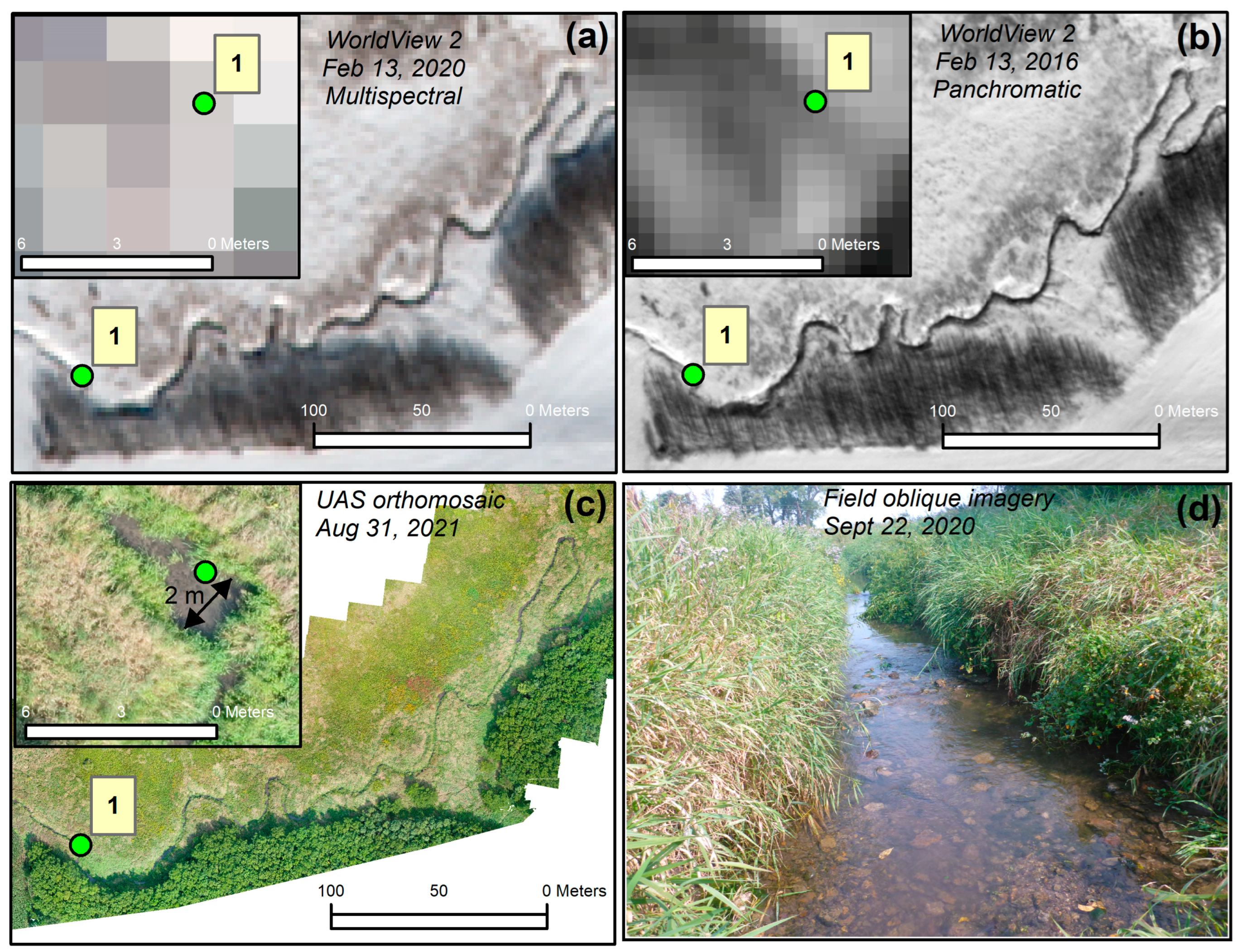
| 1 | 2.2 | YES | YES (Level 1) | NO | YES |
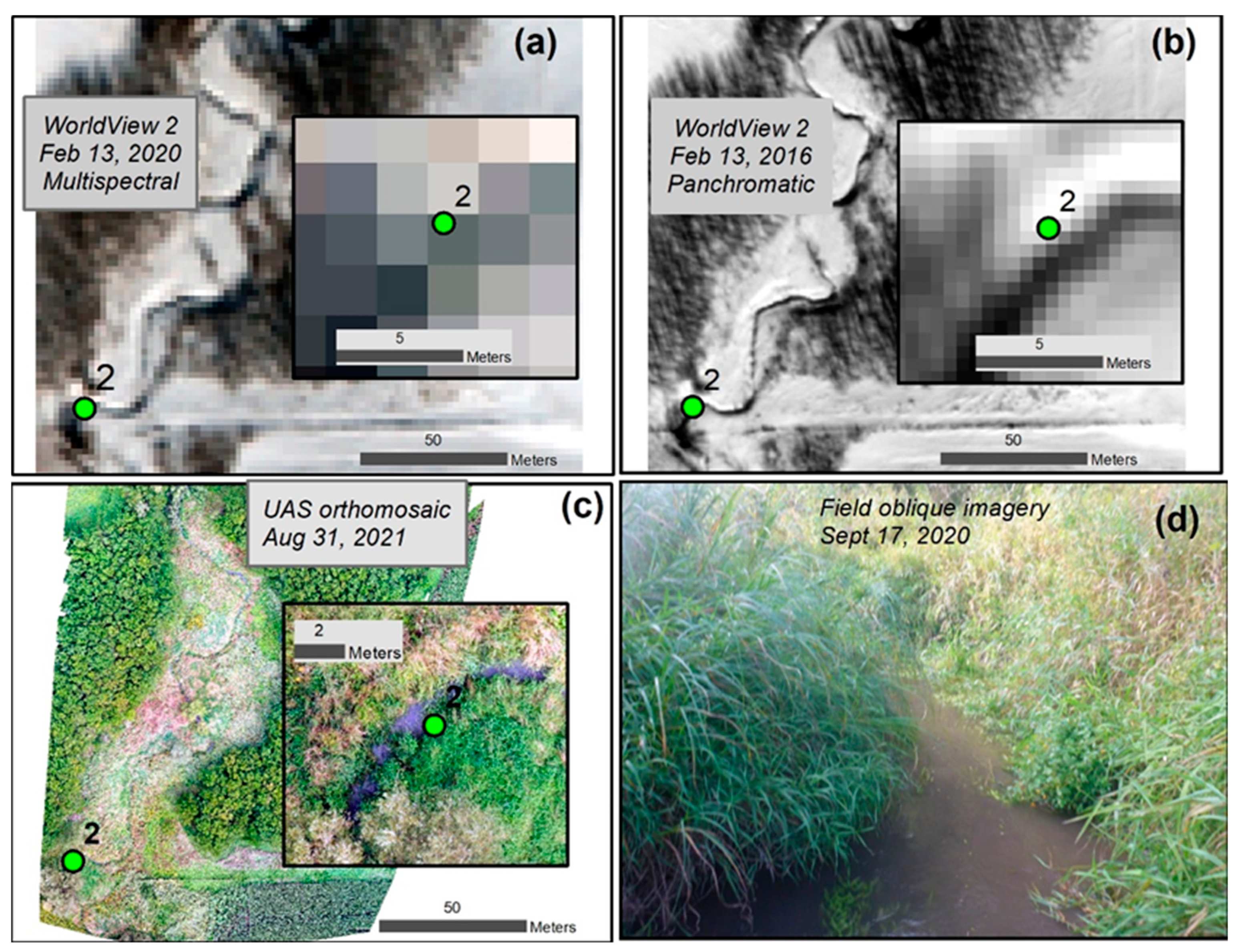
| 2 | 1.9 | YES | YES (Level 2) | YES (some bank shading) | YES |
| 3 | 4.9 | YES | YES (Level 1) | YES (some bank shading) | YES |
| 4 | 2.3 | YES | YES (Level 2) | YES | NO |
| 5 | 1.5 | YES | YES (Level 2) | YES | YES |
| 6 | 2.3 | NO | NO | YES | YES |
| 7 | 5.5 | YES | YES (Level 1) | NO | YES |
| 8 | 5.6 | YES | YES (Level 1) | NO | YES |
| 9 | - | NO (location dry) | NO | YES | YES |
| 10 | 2 | YES | YES (Level 2) | YES | YES |
| 11 | 3.4 | YES | YES (Level 1) | NO | YES |
| 12 | 1.1 | YES (watercress observed) | NO | YES | NO |
| 13 | 2.7 | YES | YES (Level 1) | NO | YES |
| 14 | 2.9 | YES | YES (Level 1) | NO | YES |
| 15 | 4 | YES | YES (Level 1) | NO | YES |
| 16 | 4.1 | YES | YES (Level 2) | YES | YES |
| 17 | 2.7 | NO (1 brown trout sampled) | NO | NO | YES |
| 18 | 4.3 | YES | YES (Level 1) | NO | YES |
| 19 | 7.1 | YES | NO | YES | NO |
| 20 | 13.7 | YES | YES (Level 1) | NO | YES |
| 21 | 6 | YES | YES (Level 1) | NO | YES |
Disclaimer/Publisher’s Note: The statements, opinions and data contained in all publications are solely those of the individual author(s) and contributor(s) and not of MDPI and/or the editor(s). MDPI and/or the editor(s) disclaim responsibility for any injury to people or property resulting from any ideas, methods, instructions or products referred to in the content. |
© 2023 by the authors. Licensee MDPI, Basel, Switzerland. This article is an open access article distributed under the terms and conditions of the Creative Commons Attribution (CC BY) license (https://creativecommons.org/licenses/by/4.0/).
Share and Cite
Mishra, N.B.; Siepker, M.J.; Simmons, G. Applying High-Resolution Satellite and UAS Imagery for Detecting Coldwater Inputs in Temperate Streams of the Iowa Driftless Region. Remote Sens. 2023, 15, 4445. https://doi.org/10.3390/rs15184445
Mishra NB, Siepker MJ, Simmons G. Applying High-Resolution Satellite and UAS Imagery for Detecting Coldwater Inputs in Temperate Streams of the Iowa Driftless Region. Remote Sensing. 2023; 15(18):4445. https://doi.org/10.3390/rs15184445
Chicago/Turabian StyleMishra, Niti B., Michael J. Siepker, and Greg Simmons. 2023. "Applying High-Resolution Satellite and UAS Imagery for Detecting Coldwater Inputs in Temperate Streams of the Iowa Driftless Region" Remote Sensing 15, no. 18: 4445. https://doi.org/10.3390/rs15184445
APA StyleMishra, N. B., Siepker, M. J., & Simmons, G. (2023). Applying High-Resolution Satellite and UAS Imagery for Detecting Coldwater Inputs in Temperate Streams of the Iowa Driftless Region. Remote Sensing, 15(18), 4445. https://doi.org/10.3390/rs15184445