Communication

Improved Amplitude-Phase Calibration Method of Nonlinear Array for Wide-Beam High-Frequency Surface Wave Radar

1
Hubei Key Laboratory of Intelligent Vision Based Monitoring for Hydroelectric Engineering, China Three Gorges University, Yichang 443002, China
2
College of Computer and Information Technology, China Three Gorges University, Yichang 443002, China
3
Hubei Zhongnan Pengli Ocean Detection System Engineering Co., Ltd., Yichang 430000, China
4
Zhuhai Marine Environment Monitoring Center Station of State Oceanic Administration, Zhuhai 519000, China
*
Author to whom correspondence should be addressed.
Remote Sens. 2023, 15(18), 4405; https://doi.org/10.3390/rs15184405
Submission received: 6 July 2023 / Revised: 31 August 2023 / Accepted: 4 September 2023 / Published: 7 September 2023

Abstract

:
The amplitude and phase errors in array elements lead to uncertainties in the estimation of arrival angles (DOA), which, in turn, affect the accuracy of current measurements for high-frequency surface wave radar (HFSWR). To address this issue, this paper proposes a passive amplitude-phase self-calibration method for a wide-beam HFSWR system with a nonlinear array. This method utilizes the aggregation of the amplitude ratio among array elements to screen reception matrices of single DOA sources. Based on the differences in reception matrices, the amplitude error is calibrated. Moreover, the cost function is calculated using the multiple signal classification (MUSIC) algorithm, and the initial phase error is first obtained after triangular array dimensionality reduction. Then, the phase error is further calibrated through quadratic-form iterative optimization. This method has been validated through simulations and real measurements. An approximately 4-day dataset obtained via HFSWR is reanalyzed in this paper. After data calibration, the radar-estimated currents were in good agreement with the buoy-measured results, with a root mean square error (RMSE) as low as 0.06 m/s and a correlation coefficient (CC) of up to 0.88. The results indicate that this method is suitable for the amplitude and phase error calibration of nonlinear arrays in wide-beam HFSWR systems.

Graphical Abstract

1. Introduction

Since the pioneering work of electromagnetic scattering from the ocean surface, high-frequency surface wave radars (HFSWR) located on the coast have been widely applied in marine environment monitoring over the world for wave, wind, and especially current measurements [1,2,3]. The resonance scattering mechanism between electromagnetic waves and the sea surface results in two discrete peaks in the Doppler spectrum [4,5]. The radial current maps can be obtained from these backscattering echoes [6].
The accuracies of the obtained current are influenced by many factors such as radio wavelength, power spectrum frequency resolution, and the direction of arrival (DOA) estimation performance of the first-order ocean echoes [7,8]. Radio wavelength and power spectrum frequency resolution can be easily determined via radar waveform parameters, while the DOA is always estimated by the multiple signal classification (MUSIC) algorithm and beamforming algorithm [9,10]. The algorithms have high resolution performance under the premise that the echo signal satisfies the hypothesis of ideal model. However, the array performances in practical applications will be significantly reduced for the array errors resulting from position, mutual coupling effect, or channel amplitude and phase errors [11]. Without effective calibration, a HF radar system not only estimates spurious directions but also provides a poor azimuth resolution for wave, wind, and especially current measurements. As a consequence, the array calibration algorithm has become increasingly important for HF radar ocean surface remote sensing.
A common method for array calibration can effectively correct the array manifold by placing a responder on the shore or ship as an auxiliary calibration source [12,13]. However, this method struggles to provide continuous real-time calibration values, and the installation and maintenance of the transponder are also relatively expensive in terms of economic costs. In recent years, the passive amplitude and phase calibration has been widely applied. Under the passive mode, without the installation of auxiliary equipment or the acquisition of prior information, self-calibration of amplitude and phase errors can be achieved by directly processing radar echo information. Meanwhile, the calibration will be approximately real-time while the ocean echo is stable. Friedlander and Weiss proposed a classical method for amplitude-phase error self-calibration by utilizing the orthogonality of noise subspace and signal subspace [14,15]. Subsequently, Solomon extended this method and took ionized meteor trajectories as single sources for passive amplitude and phase calibration [16]. In 2006, Wu Xiongbin utilized the shift-invariant antenna pairs to select the single sources in ocean echoes, and calibrated it through the maximum likelihood (ML) cost function [17]. The search for single DOA signals using shift-invariant antenna pairs is a relatively reliable method, while the maximum likelihood cost function requires multi-dimensional search for both direction of arrival and amplitude-phase error, which leads to the problem of overestimation of the parameters. In addition, not all arrays of HF radar have shift-invariant antenna pairs [18,19]. Similar to the ML method, Chen et al. proposed another appoach based on the multiple signal classification (MU) algotithm for amplitude and phase calibration using the reception matrices of single DOA sources [20]. Later, Zhao Chen validated and compared the ML method and the MU method, and the results showed that both methods can effectively improve the accuracy of ocean current estimation [21].
In summary, the passive amplitude and phase calibration method can provide better application prospects for estimating ocean current parameters for HF radar. Based on the perspective of orthogonality between noise subspace and signal subspace, this paper proposes a method for amplitude and phase calibration of nonlinear arrays in wide-beam HF radar. The reception matrices of single DOA sources are screened by the aggregation of the amplitude ratio between array elements. Combining triangular array dimensionality reduction with the MUSIC method, stable and accurate estimation of the initial phase values was achieved. To validate this method, the datasets collected with a OSMAR071G radar deployed at Pearl River Estuary in April 2021 were reanalyzed.
The article is organized as follows. Section 2 provides a description of the array signal model. The amplitude and phase calibration method is also given in this section. In Section 3, the method is tested using a simulated dataset. To validate the proposed method, four-day comparisons between radar-retrieved and buoy-measured current velocities are made in Section 4. Conclusions and perspectives on future work are presented in Section 5.

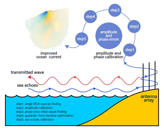
2. Array Signal Model and Amplitude and Phase Calibration Method

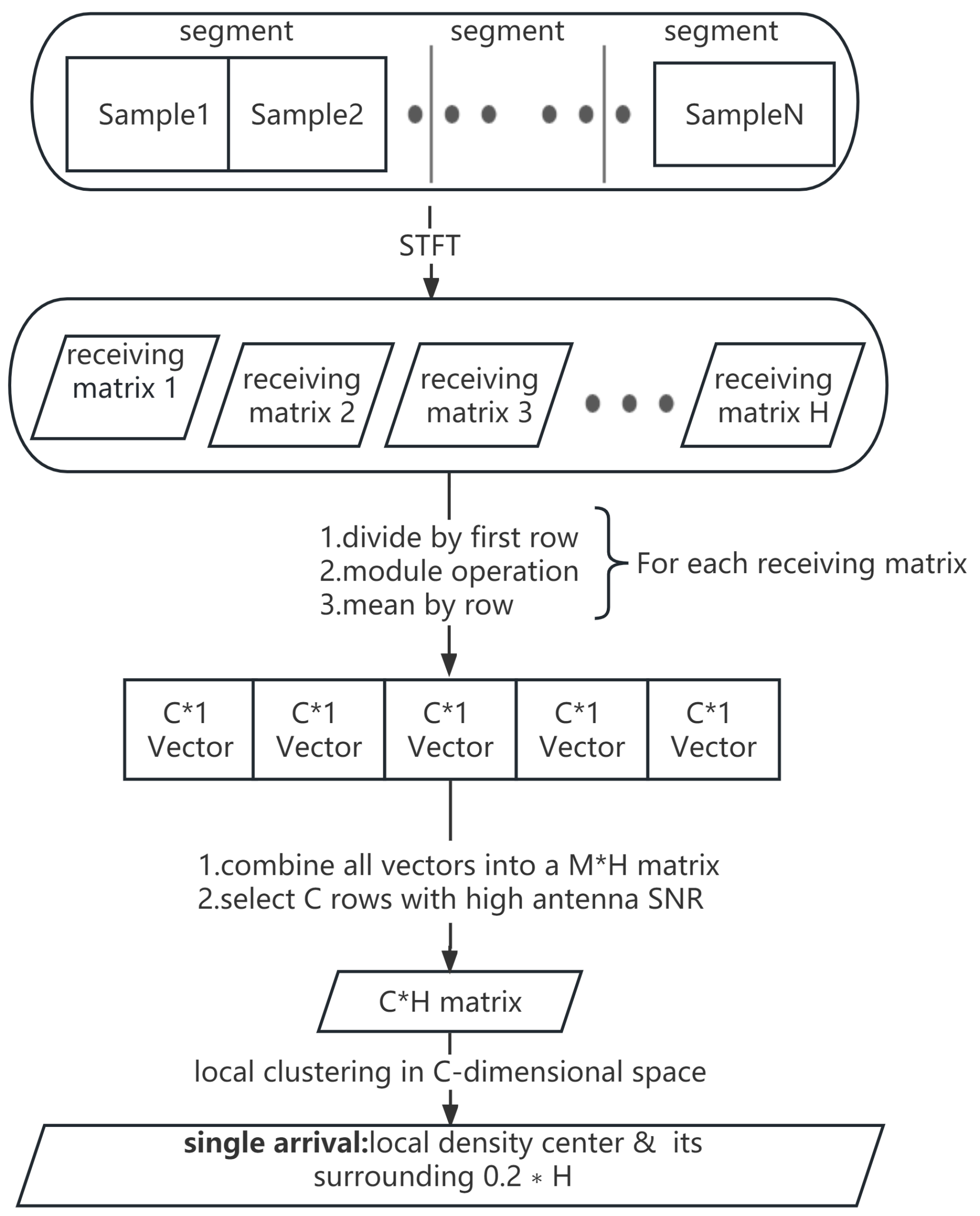
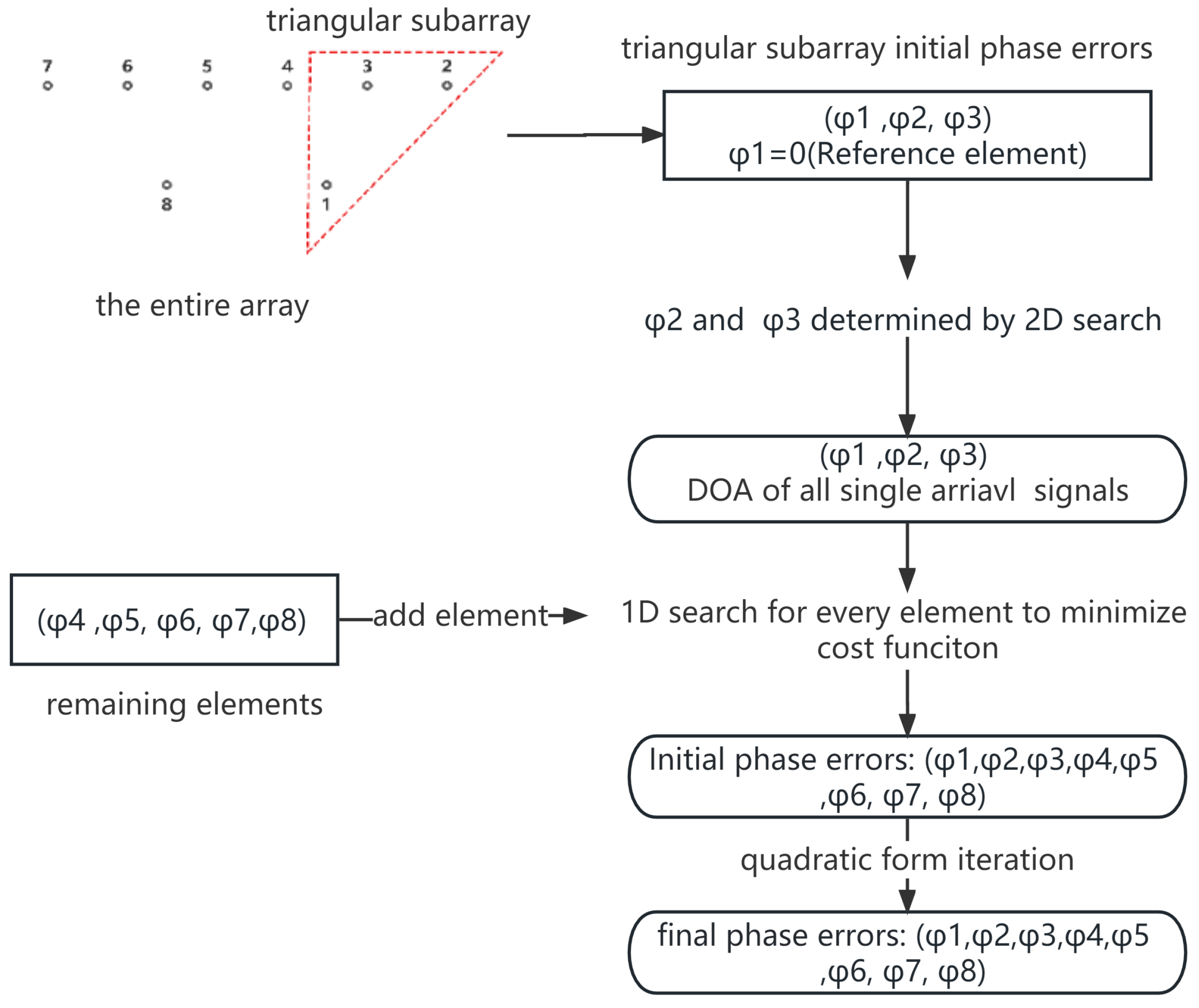
2.1. Array Signal Model

Assuming the array HF radar has M array elements, and the coordinates of array element i are ( x i , y i ) ( i = 1 , 2 M ), x 1 = 0 , y 1 = 0 . After two fast Fourier transforms (FFTs), the echo signal model on channel i can be simply described as:
z i ( m , o ) = g i e ( j φ i ) k = 1 K S k ( m , o ) a i ( θ k ) + n i ( m , o )
where m is the discrete frequency on the distance dimension; o is the Doppler frequency shift; g i and e j φ i are the amplitude and phase errors, respectively; S k represents a two-dimensional echo signal of an arrival angle of θ k ; and n i is the additive noise. The steering vector a ( θ k ) can be represented by
a ( θ k ) = [ 1 a 2 ( θ k ) a M ( θ k ) ] T ,
where a i ( θ k ) = e j 2 π λ ( x M sin θ k + y M cos θ k ) , λ is the radio wavelength.
The response of the receiving array is
X = G Φ A S + N ,
where X = [ Z 1 Z 2 Z M ) ] T , which represents an array snapshot during the coherent accumulation period; G = d i a g ( [ 1 g 1 g M ] T ) , Φ = d i a g ( [ 1 e j φ 2 e j φ M ) ] T ) , which are amplitude and phase error matrix, respectively; S = [ S 1 S 2 S k ] T , is the signal vector; N = [ n 1 n 2 n M ) ] T , is the array additive noise; and A is the theoretical manifold, A = [ a ( θ 1 ) a ( θ 2 ) a ( θ k ) ]

2.2. Amplitude and Phase Calibration Method
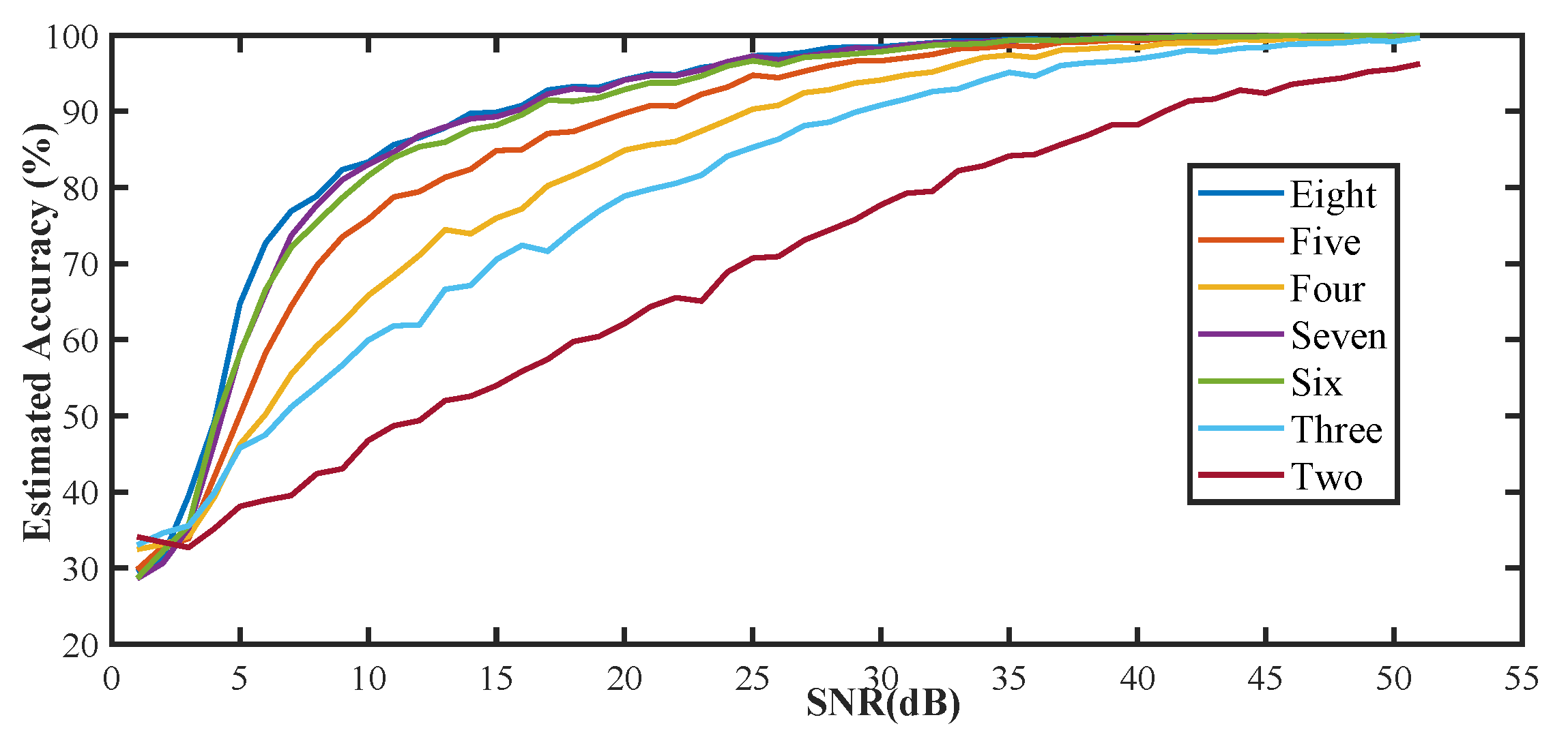
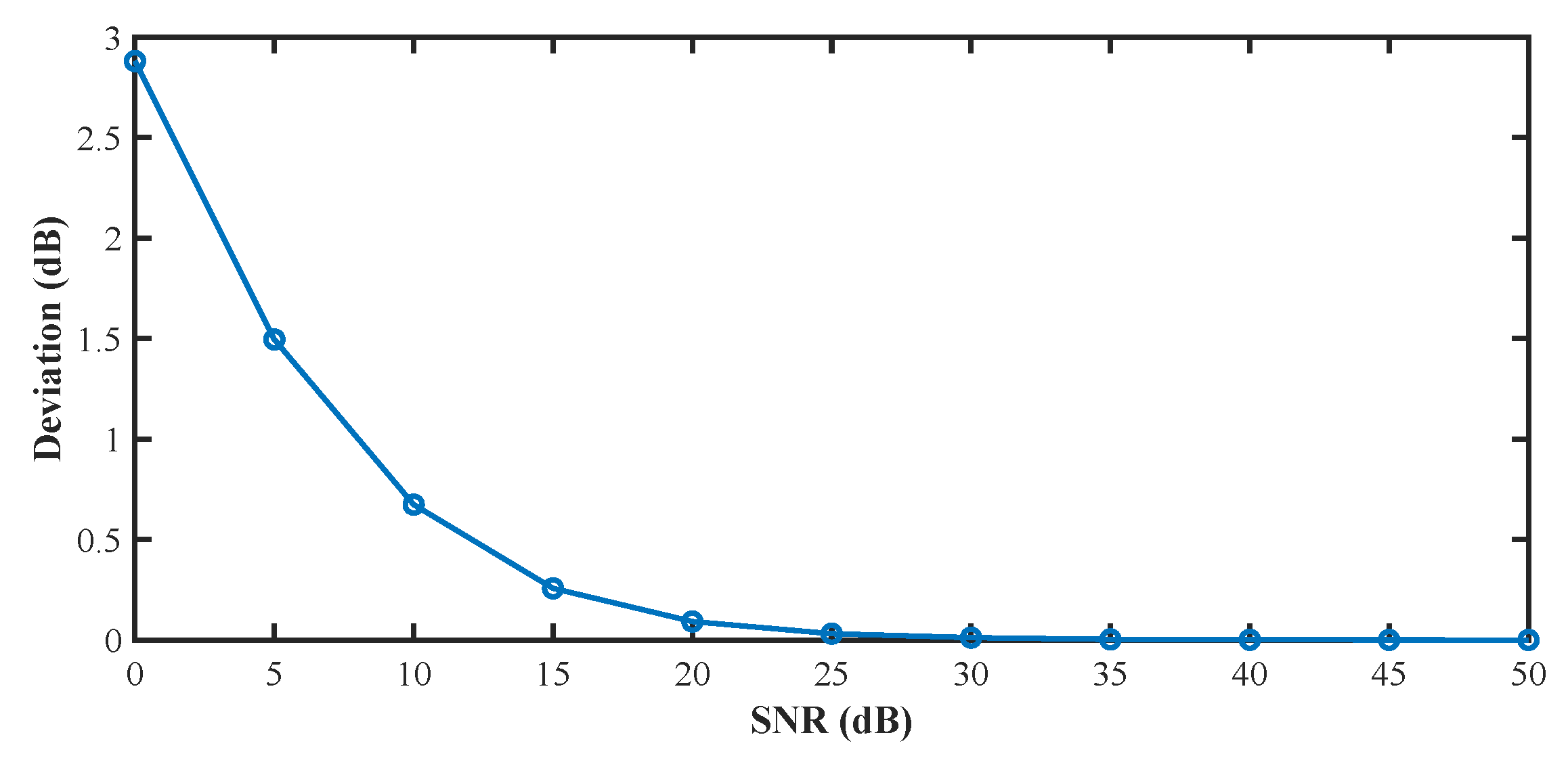
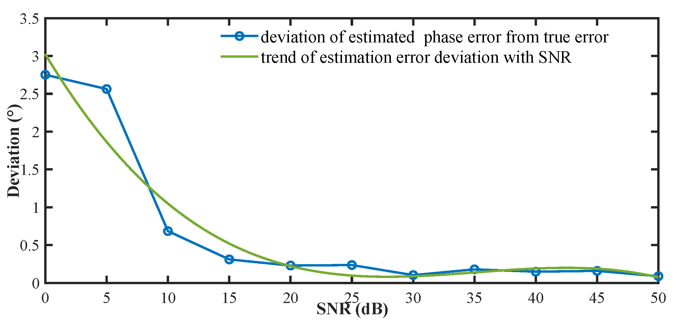
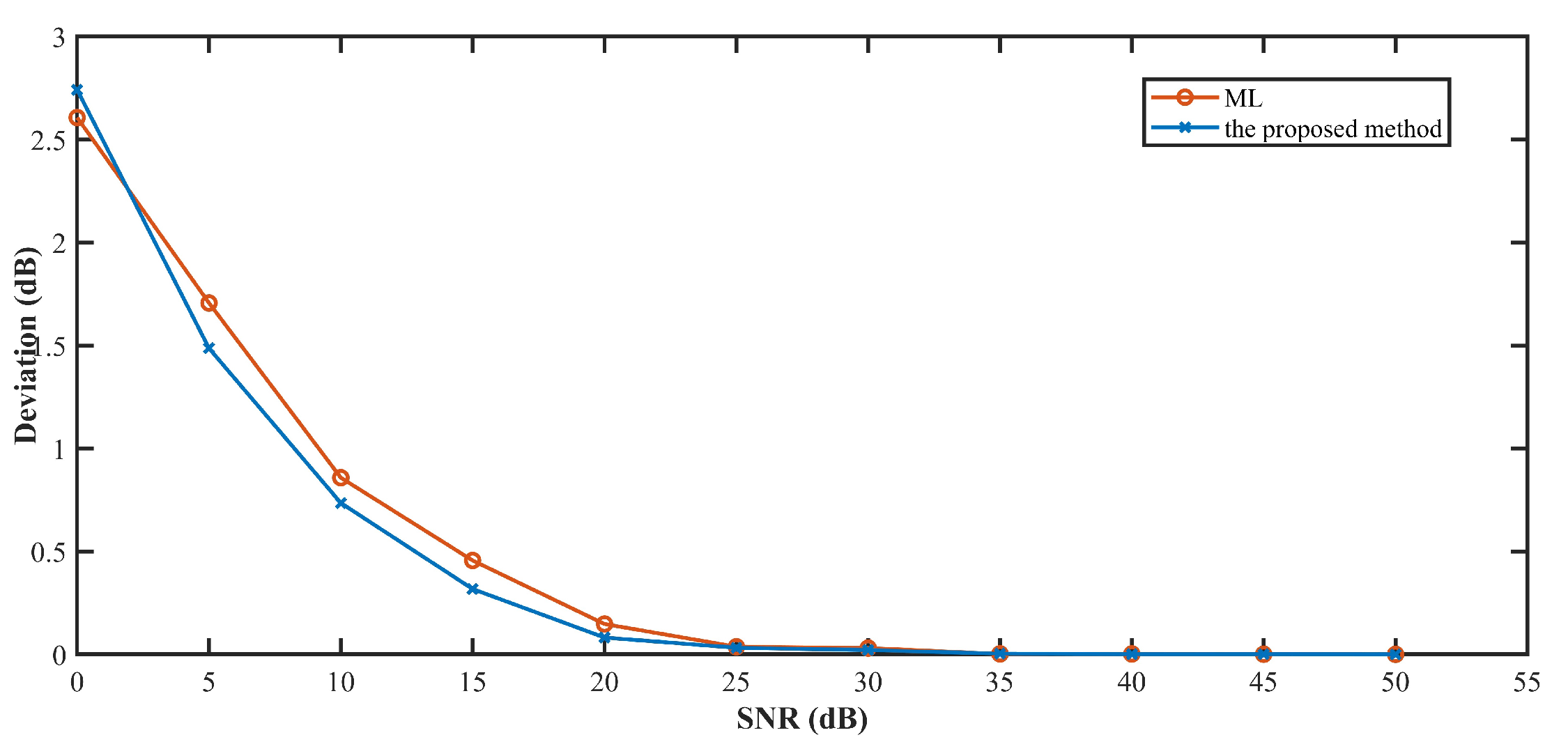
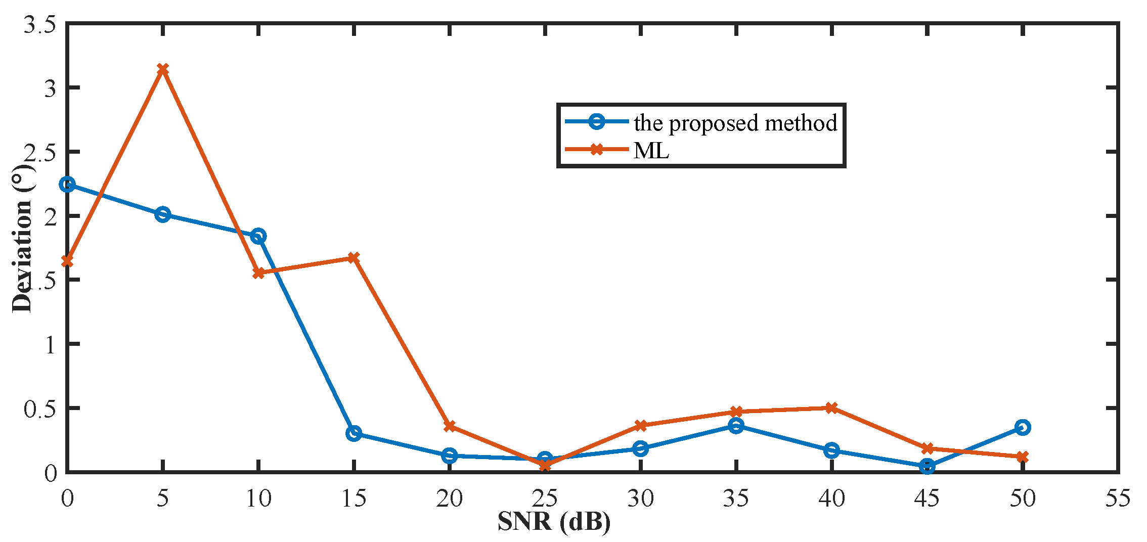
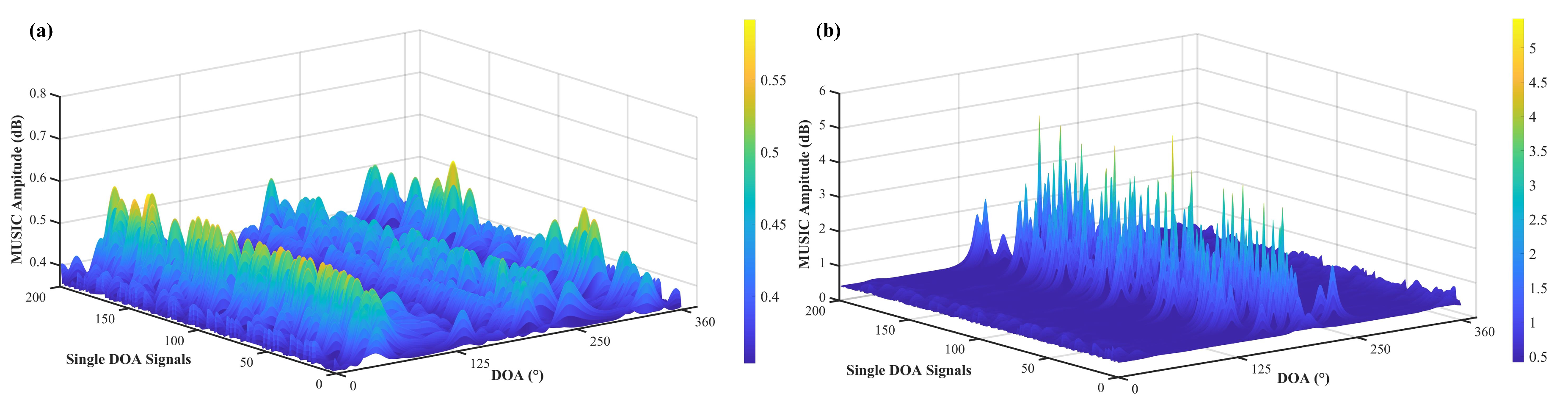
According to Equation (1), when K = 1, the two-dimensional echo is a single direction of arrival signal:
z i ( m , o ) = g i e j φ i S ( m , o ) a i ( θ ) + n i ( m , o ) .
If noise is ignored (i.e., n i ( m , o ) = 0 ), the above equation is simplified as
z i ( m , o ) = g i e j φ i S ( m , o ) a i ( θ ) .
Due to g 1 = e j φ 1 = a 1 ( θ ) = 1 ,
z 1 ( m , o ) = g 1 e j φ 1 S ( m , o ) a 1 ( θ ) = S ( m , o ) .
Therefore, for a specific single direction of arrival signal, the amplitude error of array element i is
g i = z i z 1 = g i e j φ i s ( m , o ) a i ( θ ) s ( m , o ) = g i e j φ i a i ( θ ) .
In fact, noise always exists, which results in different amplitude errors for different single direction of arrival signals. Taking the statistical average of the amplitude errors of multiple single arrival angles can further improve accuracy:
g i ˜ = l t z i ( l , t ) 2 l t z 1 ( l , t ) . 2
After amplitude error correction, the array covariance matrix corresponding to any single arrival signal can be expressed as
R = E [ X ( t ) X ( t ) H ] = Φ a ( θ l ) σ l 2 a H ( θ l ) Φ H + σ n 2 I ,
where ( . ) H is the conjugate transposition; σ l 2 and σ n 2 are the signal power and noise power, respectively; and X ( t ) is the recieved matrices corresponding to signal l. Decompose on R:
R = m = 1 M λ m μ m μ m H = E s ( l ) Λ s E s H ( l ) + E n ( l ) Λ n E n H ( l ) ,
where E n H ( l ) is the noise subspace.
Due to E n H ( l ) [ Φ a ( θ l ) ] = 0 , the MUSIC sum cost function based on the orthogonal principle of noise subspace under single direction of arrival conditions is [22]
P = a r g min Φ , θ l l = 1 L E n H ( l ) Φ a ( θ l ) 2 .
Based on the eigenvalue structure of the cost function P, sufficient reception matrices of single DOA sources can be selected to ensure the universality and anisotropy of the arrival angle distribution in the case of uncertain single DOA sources.
When K 1 ,
z i z 1 = g i e j φ i k = 1 K S k ( m , o ) a i ( θ k ) k = 1 K S k ( m , o ) .
Compare (12) with (7), for single DOA sources, the amplitude ratio between two antennae is exactly the amplitude error g i if noise is ignored, while it will concentrate around the amplitude error if noise is considered. However, for multi-DOA sources, the ratio does not show aggregation an effect since the modulus of ratio is random for the uncertainty of the arrival angle.
The aggregation effect mentioned above can be used for the selection of single arrival signals. Ideally, only two antennae are needed to find the single direction of arrival signal. However, the signal-to-noise ratio (SNR) for HF radar is usually around 20 dB or even lower. Therefore, if only two antennae are used, the above clustering effect will be weakened. Here, multiple antennae for joint estimation are considered.
A method is proposed by which to construct and screen reception matrices of single DOA sources in this article, utilizing the aggregation effect for multiple antennae mentioned above. Without considering phase information, the single DOA sources can be obtained solely through amplitude information, which means that there are no specific requirements on the antenna array layout. Figure 1 shows the algorithm flow. The steps are as follows.
Step 1: Divide sampling frames into multiple segments.
Step 2: Build a reception matrix via short-rime Fourier transform (STFT) for each segment. The frequency of the reception matrix corresponds to a two-dimensional frequency point after two FFTs. Set the number of receiving matrices as H.
Step 3: Construct a multidimensional spatial point set. For the reception matrix, divide each row of the matrix by the reference element row (generally the first row) and then take the modulus to form a new matrix. Average the matrix by rows to form a column vector of M * 1 . Combine all vectors into a M*H matrix. Select C (C > 2) rows with high-antenna SNR; then, a set of C-dimensional spatial points of size H will be formed for all the reception matrices.
Step 4: Find the single DOA sources by local clustering. Calculate the sum of squares of the distances from p i to the points which are the nearest 0.2 * H points, denoted as s u m _ p i . When taking the minimum value of s u m _ p i , the p i is the local density center. p i and its surrounding 0.2 * H points are identified as a single arrival.
To approximate the true phase error and the corresponding single arrival signal azimuth, it is necessary to optimize the minimum value of Equation (11). Based on the maximum likelihood cost function of the snapshot, the shift-invariant antenna pairs can be used to accurately determine whether a certain snapshot of the two-dimensional echo is a single arrival. However, due to the eigenvalue structure of the cost function P, the single arrival signal is not a specific snapshot but a reception matrix composed of continuous snapshots; and for L reception matrices, if the arrival angle distribution is limited to a too small interval, it will lead to ambiguity in the calibration values. Therefore, in the case of uncertain single DOA sources, sufficient reception matrices should be screened to ensure the universality and anisotropy of the arrival angle distribution.
In addition, to find a more accurate initial value of phase error, a triangular array dimensionality reduction and initial value-finding method based on the sum MUSIC cost function was designed. Figure 2 shows the algorithm flow. By constructing triangular subarrays and gradually adding elements, the complexity of the initial value estimation in Equation (11) will be reduced. Moreover, whether a signal is strictly a single arrival or not is not a necessary condition based on the idea of least squares. The setailed steps are as follows.
Step 1: Construct a nonlinear subarray (triangular subarray) with phase errors of ( φ 1 , φ 2 , φ 3 ) . φ 1 is the reference element phase error (typically set to 0). φ 2 and φ 3 are ergodically searched with a fixed step through [ π , π ] [23].
Step 2: Search for the arrival angle θ as well as the corresponding MUSIC spectral value.
Step 3: Obtain the initial phase error values of the array ( φ 1 , φ 2 , φ 3 ) and the arrival angles of each single source via Equation (11).
Step 4: Add the phase error of an adjacent array element with a fixed step from [ π , π ] to the array ( φ 1 , φ 2 , φ 3 ) and substitute the phase error values of the newly generated subarray determined via each traversal into Equation (11). Determine the phase error of the new array element by minimizing the cost function. Add array elements one by one until all the initial errors are determined.
Step 5: Calculate the optimal solution of phase error after quadratic-form iteration via Equation (11).

3. Simulation

Figure 3 shows a schematic diagram for an antenna, which has an eight-element dual nonlinear array. The horizontal spacing d 1 of array elements for the first row is set to be 18 m, for the second row, d 2 , it is 36 m, and the vertical spacing d 3 between the two rows is 15 m.
Assuming the operating frequency of the radar is 8 MHz. Simulate the reception matrix corresponding to the two-dimensional echo spectral points using an 8 * 32 complex matrix. Amplitude errors from g 1 to g 8 are [0, 1.2, 2.85, −3, 0.92, 3.1, −2,5], respectively, and phase errors ranging from φ 1 to φ 8 are [ 0 ° , 25 ° , 37.2 ° , 78 ° , 120.5 ° , 31 ° , 50 ° , 77 ° ]. The flow pattern resolution of the spatial array used for estimating azimuth is 1 ° , the number of two-dimensional ocean echo signals is 2000, the arrival angle is randomly distributed between 1 and 4, and the single source ratio is one third. The triangular subarray used for estimating the initial value of phase error is 1-4-8, and the subsequent expanded antenna sequence is 2-3-5-6-7. Perform 50 Monte Carlo experiments using the method described in 2.2 under the SNR of 0 dB ∼ 50 dB and take the average of the calculated results as the amplitude and phase error result.
The accuracies of estimating single DOA sources when selecting different numbers of array elements under different signal-to-noise ratio conditions are shown in Figure 4. To maintain high accuracy, a sufficiently high signal-to-noise ratio is required for selecting single arrival sources from fewer array elements, while at lower signal-to-noise ratios, a large number of the array elements is needed. However, an increase in the number of antennae will lead to an increase in the computational complexity of the algorithm, and when the number of antennae reaches a certain threshold beyond which the improvement in accuracy is no longer significant. Therefore, practically, it is common to select a small number of array elements (≥3) with high SNR to estimate single DOA sources.
Figure 5 and Figure 6 show the trends of the estimation deviations of the amplitude error and phase error under different SNR conditions. As the signal-to-noise ratio increases, the deviation of amplitude error estimation decreases sharply. While the deviation of phase error estimation is not significantly reduced, it still shows a downward trend. Moreover, when the SNR is higher than 10 dB, the phase error estimation deviation is <1° and the amplitude error is ≤0.7 dB.
To further evaluate the performance of the proposed method, the impact of antenna position errors were taken into account. In Figure 3, the coordinates of antenna 1 changed from (−27, −15) to (−27.2, −15), the coordinates of antenna 4 changed from (−36, 0) to (−36.2, 0), and the coordinates of antenna 8 changed from (−63, −15) to (−63.1, −15). Although these errors are often neglected in engineering when the deviations are small, they still have a certain impact on amplitude and phase calibration.
Figure 7 and Figure 8 show the trends of estimation deviations for amplitude and phase errors under different signal-to-noise ratio (SNR) conditions for both the existing maximum likelihood (ML) method and the method proposed in this paper. Clearly, both the ML method and the proposed method demonstrate good calibration performance when the SNR is high (>20 dB). However, when the SNR is low, the ML method exhibits greater fluctuations, resulting in unstable calibration performance. This is because the ML method requires specific array layouts and the determination of the (or more) single arrival signals when searching for the initial values, which imposes certain limitations.

4. Validation

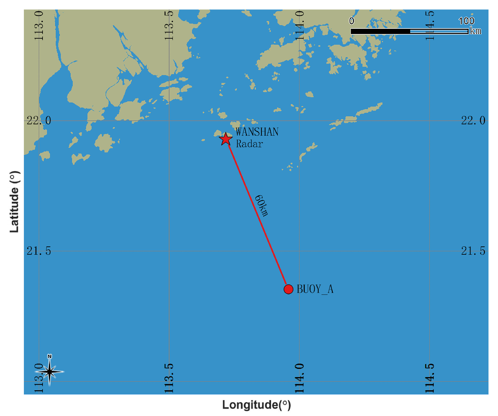
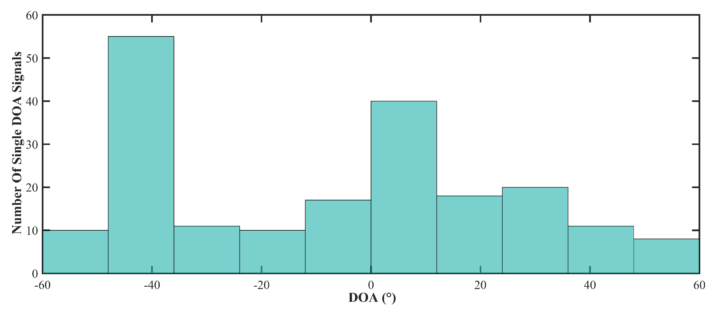
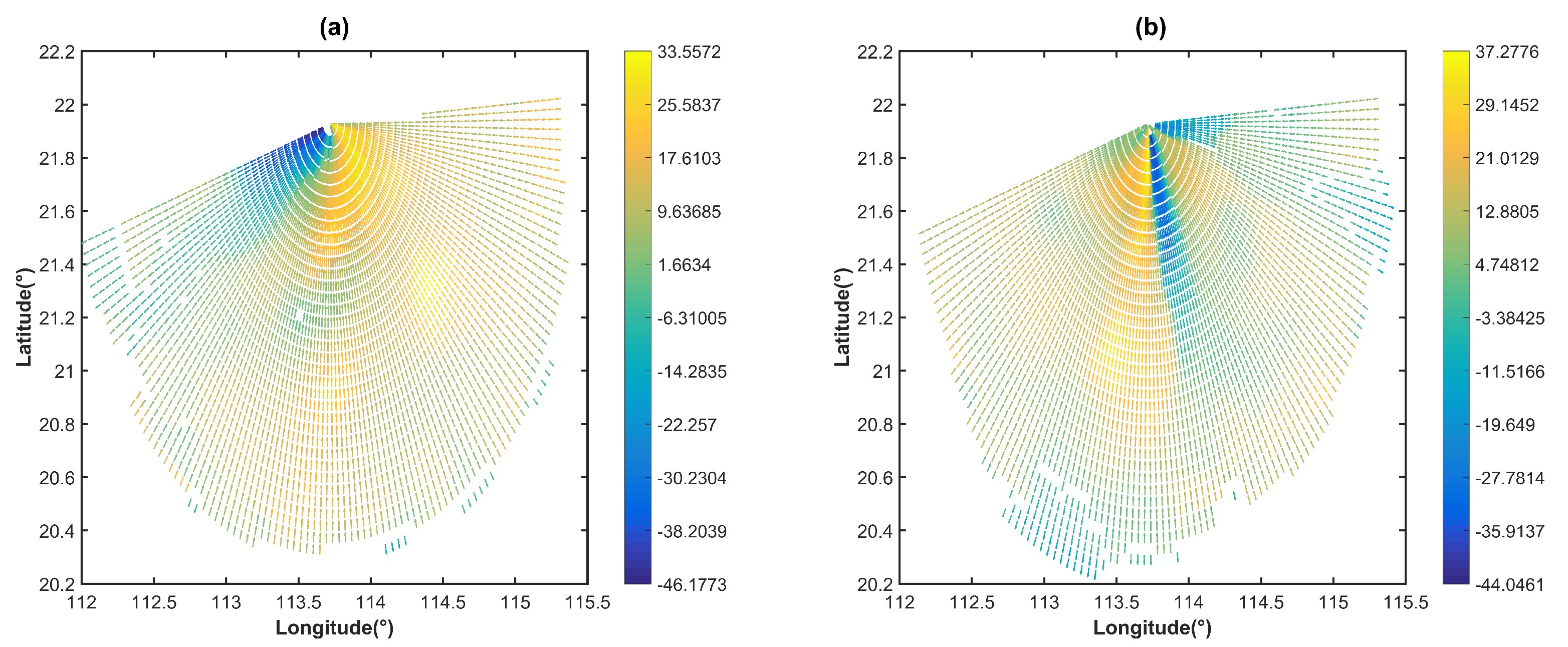
4.1. Equipment and Setup

From 30 April to 3 May 2021, an experiment was carried out to validate the amplitude-phase calibration method at Pearl River Estuary via a OSMAR071G radar. To realize monostatic operation, the radar employs frequency-modulated interrupted continuous wave (FMICW) chirps for radio energy radiation and uses a nonlinear array-receiving antenna, as shown in Figure 3, to receive ocean echoes. The radar waveform parameters are listed in Table 1.
By measuring the projection of surface currents at any point on the sea surface towards the radar direction, radial currents can be obtained. A wave buoy was deployed about 60 km from the OSMAR071G. The positions of the radar and buoy are shown in Figure 9. The buoy-derived current measurements are presented as “sea-truth”. For convenience, both the buoy and radar produce current velocity every 10 min for comparison.

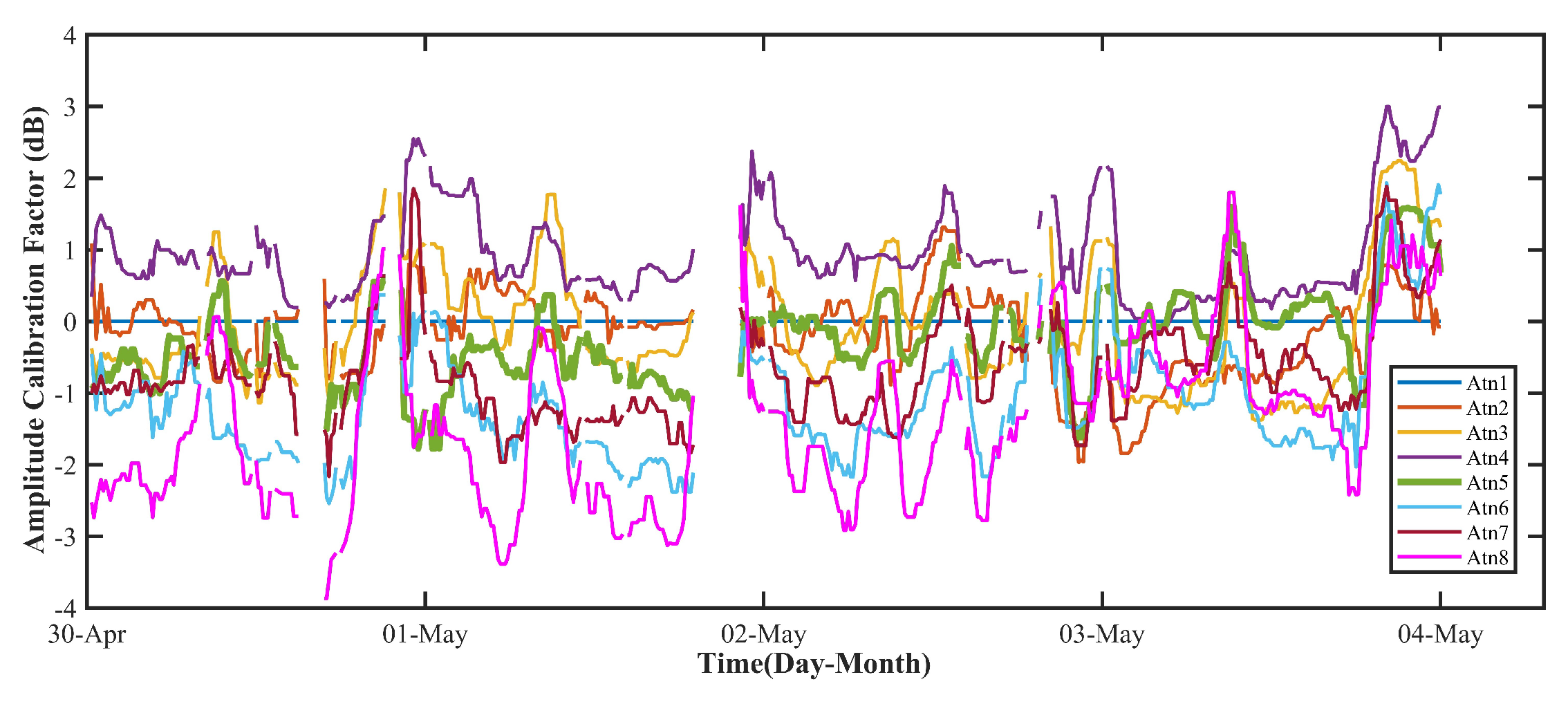
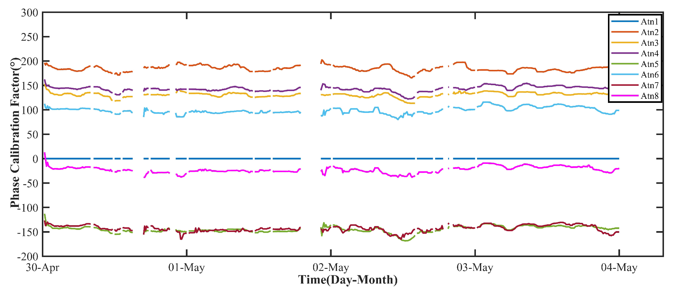
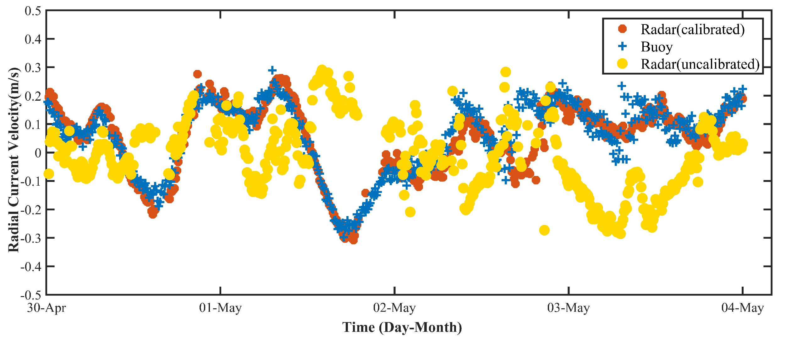
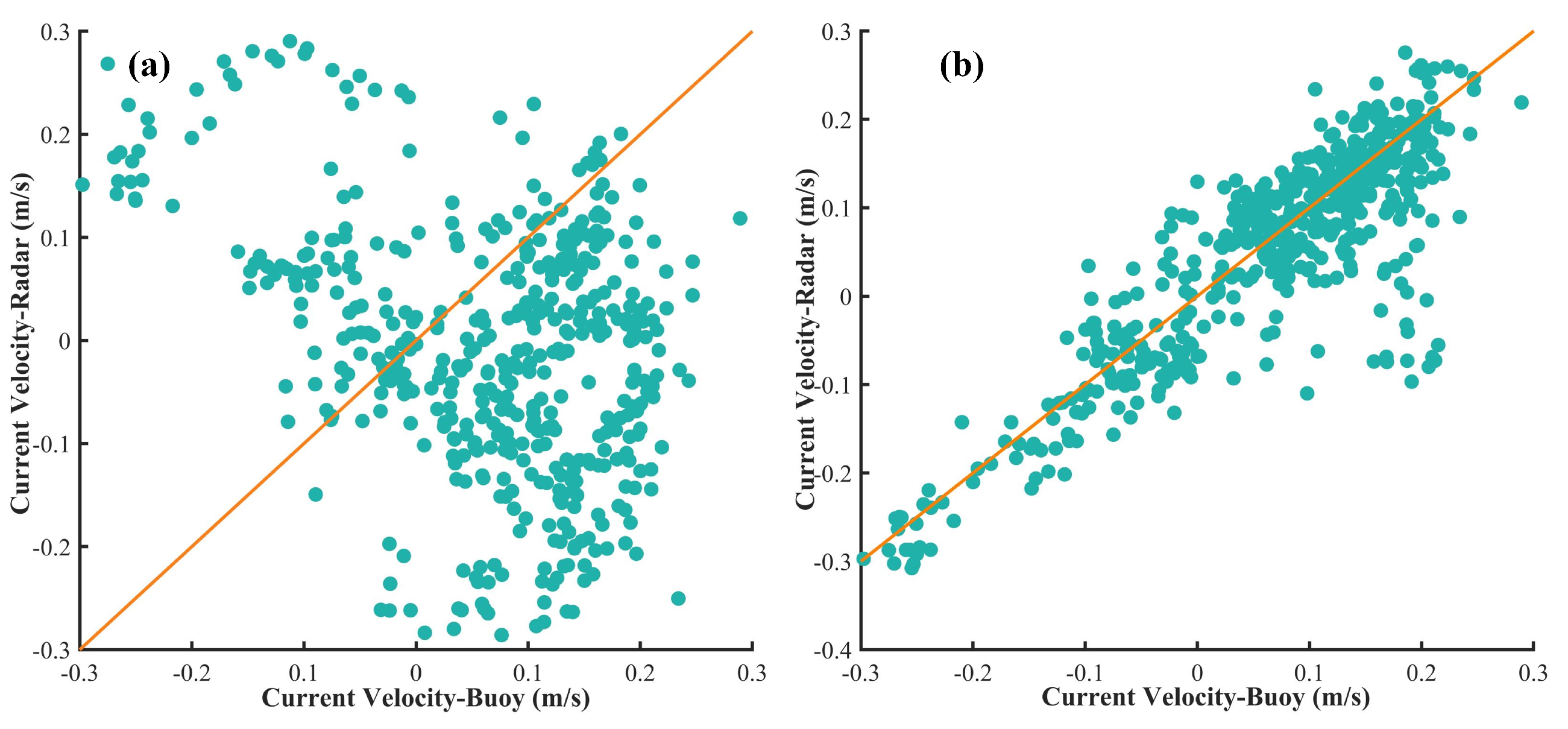
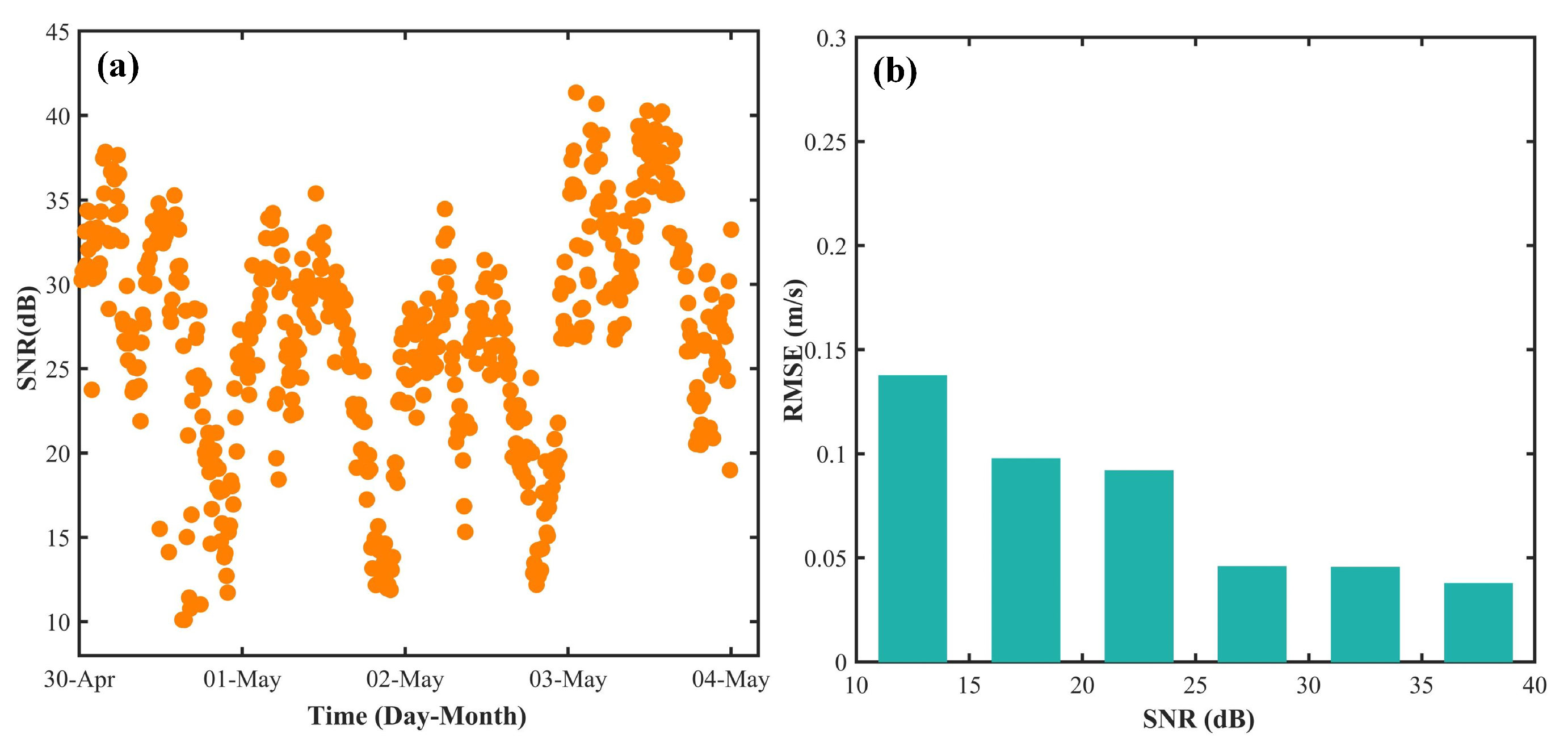
4.2. Observations and Discussion

We performed amplitude and phase calibration on echo data based on the method proposed in this article. Figure 10 and Figure 11 show the amplitude and phase calibration factors, respectively. Due to the weak signal-to-noise ratio (SNR) of the echo information from the single arrival angle used for calibration (below 12 dB), the datasets from 19:00 on 1 May to 22:00 on 1 May are not considered here.
A total of 200 single sources were selected at 14:30 on 1 May for amplitude and phase calibration via the method proposed in this article; then, we performed a MUSIC estimation on these 200 calibrated sources. Figure 8b and Figure 12a show the uncalibrated and calibrated MUSIC estimation spectra, respectively. There are many pseudo peaks in the uncalibrated MUSIC spectrum. It will be difficult to obtain the correct DOA since the spectrum has low SNR and wide beams, while the calibrated MUSIC spectrum, with high SNR, generally only has one peak and needle-like narrow beams, which makes it easy to determine the DOA.
Figure 13 shows the histogram statistics of the MUSIC-estimated arrival angles for the 200 single sources mentioned above after amplitude and phase calibration. Obviously, the arrival angle distribution of a single source is within the range of [−60, 60] centered on the array normal, which is also the radiation field angle range of the electromagnetic waves for the radar deployed at Wanshan. This demonstrates the rationality of the arrival angle distribution of a single source and further verifies the accuracy of amplitude and phase error estimation.
Comparisons of current velocity between the RADAR and the wave buoy have been undertaken. The comparison of radial flow fields of ocean currents with and without calibration at 9:10 am on 3 May is displayed in Figure 14. Due to the post-processing involved in ocean current inversion, the flow fields appear relatively smooth and well-defined under both calibrated and uncalibrated conditions. The radial flow field obtained from calibrated data gradually moves away from the radar as the longitude decreases, while the radial flow field obtained from uncalibrated data exhibits a very chaotic distribution in terms of flow velocity and direction. The time series are shown in Figure 15, including the buoy-measured results (blue-plus sign), the Radar-estimated results using the uncalibrated data (yellow-circle), and the Radar-estimated results using the data calibrated via the method proposed in this article (red-asterisk). The statistical characteristics are summarized in Table 2. Compared with the uncalibrated results, the current velocities extracted from the RADAR using the calibrated data agree better with the buoy-derived current measurements, with a CC of 0.88, an RMSE of 0.06 m/s and a mean difference (MD) of 0.05 m/s. The scatter plots of the uncalibrated and calibrated results are shown in Figure 16a and Figure 16b, respectively.
The signal-to-noise ratio (SNR) time series for the radar is shown in Figure 17a. The SNR varied between 10 and 40 dB. The relationship between the RMSE of the current measurements and SNR is also shown in Figure 17b. Obviously, the RMSE of the current velocities is less than 0.14 m/s and decreases with the increase in SNR.

5. Conclusions

An improved amplitude-phase self-calibration nonlinear array method based on a wide-beam HF radar system is proposed in this paper. As well as a simulation validation, a nearly four-day observation and intercomparison based on the OSMAR071G radar and buoy installed at Pearl River Estuary along the coast of Shen Zhen province in China has been analyzed in detail. The results indicate that the radar-derived measurements, after calibrating the echo data using the proposed method, have good agreement with the buoy-measured current velocity. To further validate the effectiveness of this method, we will consider the datasets under different sea conditions.

Author Contributions

Conceptualization, W.F. and H.L.; methodology, W.F. and H.L.; software, W.F. and S.Y.; validation, H.L. and Z.C.; formal analysis, H.L. and F.W.; investigation, W.F.; resources, Z.C. and Y.H.; writing—original draft preparation, W.F. and H.L.; supervision, H.L.; project administration, H.L.; funding acquisition, H.L. All authors have read and agreed to the published version of the manuscript.

Funding

This research was funded in part by Hubei Provincial Department of Science and Technology under grant 2022CFB786, and in part by Yichang City Science and Technology Bureau under grant A23-2-013.

Data Availability Statement

Not applicable.

Acknowledgments

The authors are grateful to the Hubei Zhongnan Pengli Ocean Detection System Engineering Co., Ltd., and the Zhuhai Marine Environment Monitoring Center Station of State Oceanic Administration for providing data resourses.

Conflicts of Interest

The authors declare no conflict of interest.

References

  1. Zhao, C.; Deng, M.; Chen, Z.; Ding, F.; Huang, W. Ocean Wave Parameters and Nondirectional Spectrum Measurements Using Multifrequency HF Radar. IEEE Trans. Geosci. Remote Sens. 2022, 60, 4204413. [Google Scholar] [CrossRef]
  2. Bourg, N.; Molcard, A. Northern boundary current variability and mesoscale dynamics: A long-term HF RADAR monitoring in the North-Western Mediterranean Sea. Ocean Dyn. 2021, 71, 851–870. [Google Scholar] [CrossRef]
  3. Lai, Y.; Zhou, H.; Wen, B. Surface Current Characteristics in the Taiwan Strait Observed by High-Frequency Radars. IEEE J. Ocean. Eng. 2016, 42, 449–457. [Google Scholar] [CrossRef]
  4. Zhao, C.; Chen, Z.; He, C.; Xie, F.; Chen, X. A Hybrid Beam-Forming and Direction-Finding Method for Wind Direction Sensing Based on HF Radar. IEEE Trans. Geosci. Remote. Sens. 2018, 56, 6622–6629. [Google Scholar] [CrossRef]
  5. Crombie, D.D. Doppler Spectrum of Sea Echo at 13.56 Mc./s. Nature 1955, 175, 681–682. [Google Scholar] [CrossRef]
  6. Li, M.; Zhang, L.; Wu, X.; Yue, X.; Emery, W.J.; Yi, X.; Liu, J.; Yang, G. Ocean Surface Current Extraction Scheme With High-Frequency Distributed Hybrid Sky-Surface Wave Radar System. IEEE Trans. Geosci. Remote. Sens. 2018, 56, 4678–4690. [Google Scholar] [CrossRef]
  7. Lai, Y.; Zhou, H.; Zeng, Y.; Wen, B. Accuracy Assessment of Surface Current Velocities Observed by OSMAR-S High-Frequency Radar System. IEEE J. Ocean. Eng. 2017, 43, 1068–1074. [Google Scholar] [CrossRef]
  8. Zhang, Z.; Wen, F.; Shi, J.; He, J.; Truong, T.K. 2D-DOA Estimation for Coherent Signals via a Polarized Uniform Rectangular Array. IEEE Signal Process. Lett. 2023, 30, 893–897. [Google Scholar] [CrossRef]
  9. Yang, S.; Ke, H.; Wu, X.; Tian, J.; Hou, J. HF radar ocean current algorithm based on MUSIC and the validation experiments. IEEE J. Ocean. Eng. 2006, 30, 601–618. [Google Scholar] [CrossRef]
  10. Wang, X.; Guo, Y.; Wen, F.; He, J.; Truong, T.K. EMVS-MIMO Radar with Sparse Rx Geometry: Tensor Modeling and 2D Direction Finding. IEEE Trans. Aerosp. Electron. Syst. 2023. Early Access. [Google Scholar] [CrossRef]
  11. Barrick, D.E.; Lipa, B.J. Correcting for distorted antenna patterns in CODAR ocean surface measurements. IEEE J. Ocean. Eng. 1986, 11, 304–309. [Google Scholar] [CrossRef]
  12. Chen, Z.; Zhang, L.; Zhao, C.; Li, J. Calibration and Evaluation of a Circular Antenna Array for HF Radar Based on AIS Information. IEEE Geosci. Remote. Sens. Lett. 2019, 17, 988–992. [Google Scholar] [CrossRef]
  13. Paduan, J.D.; Kim, K.C.; Cook, M.S.; Chavez, F.P. Calibration and Validation of Direction-Finding High-Frequency Radar Ocean Surface Current Observations. IEEE J. Ocean. Eng. 2007, 31, 862–875. [Google Scholar] [CrossRef]
  14. Friedlander, B.; Weiss, A.J. Direction Finding in the Presence of Mutual Coupling. IEEE Trans. Antennas Propag. 1991, 39, 273–284. [Google Scholar] [CrossRef]
  15. Friedlander, B.; Weiss, A.J. Performance of direction-finding systems with sensor gain and phase uncertainties. Circuits Syst. Signal Process. 1993, 12, 3–35. [Google Scholar] [CrossRef]
  16. Solomon, I.S.D.; Gray, D.A.; Abramovich, Y.I.; Anderson, S.J. Over-the-horizon radar array calibration using echoes from ionised meteor trails. Radar Signal Process. IEE Proc. F 1998, 145, 173–180. [Google Scholar] [CrossRef]
  17. Xiongbin, W.; Feng, C.; Zijie, Y.; Hengyu, K. Broad Beam HFSWR Array Calibration Using Sea Echoes. In Proceedings of the 2006 CIE International Conference on Radar, Shanghai, China, 16–19 October 2006. [Google Scholar]
  18. Barrick, D.; Snider, J. The statistics of HF sea-echo Doppler spectra. IEEE Trans. Antennas Propag. 1977, 25, 19–28. [Google Scholar] [CrossRef]
  19. Rockah, Y.; Messer, H.; Schultheiss, P.M. Localization performance of arrays subject to phase errors. IEEE Trans. Aerosp. Electron. Syst. 1988, 24, 402–410. [Google Scholar] [CrossRef]
  20. Chen, Z.; Zeng, G.; Zhao, C.; Zhang, L. A Phase Error Estimation Method for Broad Beam High-Frequency Radar. IEEE Geosci. Remote Sens. Lett. 2015, 12, 1526–1530. [Google Scholar] [CrossRef]
  21. Zhao, C.; Chen, Z.; Zeng, G.; Zhang, L. Evaluating Two Array Autocalibration Methods with Multifrequency HF Radar Current Measurements. J. Atmos. Ocean. Technol. 2015, 32, 1088–1097. [Google Scholar] [CrossRef]
  22. Schmidt, R.; Schmidt, R.O. Multiple emitter location and signal parameter estimation. IEEE Trans. Antennas Propag. 1986, 34, 276–280. [Google Scholar] [CrossRef]
  23. Wen, F.; Shi, J.; He, J.; Truong, T.K. 2D-DOD and 2D-DOA Estimation Using Sparse L-Shaped EMVS-MIMO Radar. IEEE Trans. Aerosp. Electron. Syst. 2023, 59, 2077–2084. [Google Scholar] [CrossRef]
Figure 1. Algorithm flowchart for single DOA signals searching.
Remotesensing 15 04405 g001
Figure 2. Algorithm flowchart for finding the initial value of phase errors.
Remotesensing 15 04405 g002
Figure 3. Array diagram.
Remotesensing 15 04405 g003
Figure 4. Single DOA source estimation accuracy for different number of arraies.
Remotesensing 15 04405 g004
Figure 5. Estimation deviations of amplitude error.
Remotesensing 15 04405 g005
Figure 6. Estimation deviations of phase error.
Remotesensing 15 04405 g006
Figure 7. Estimation deviations of amplitude error for the ML method and the proposed method.
Remotesensing 15 04405 g007
Figure 8. Estimation deviations of phase error for the ML method and the proposed method.
Remotesensing 15 04405 g008
Figure 9. Map showing positions of radars and the wave buoy.
Remotesensing 15 04405 g009
Figure 10. Amplitude calibration factor.
Remotesensing 15 04405 g010
Figure 11. Phase calibration factor.
Remotesensing 15 04405 g011
Figure 12. MUSIC estimation spectra: (a) uncalibrated; (b) calibrated. The X-, Y-, and Z-axis represent the azimuth angle, different single DOA sources, and the MUSIC power spectral density, respectively.
Remotesensing 15 04405 g012
Figure 13. The histogram statistics of MUSIC-estimated arrival angles for the 200 single DOA sources mentioned above after amplitude and phase calibration.
Remotesensing 15 04405 g013
Figure 14. Radial flow field diagram of ocean current (a) calibrated; (b) uncalibrated.
Remotesensing 15 04405 g014
Figure 15. Current velocity time series obtained from the RADAR and the wave buoy.
Remotesensing 15 04405 g015
Figure 16. Scatter plot of current velocities for (a) uncalibrated (b) calibrated data.
Remotesensing 15 04405 g016
Figure 17. (a) Mean SNR series of the radar Doppler spectra. (b) RMSE of the radar measurements against SNR.
Remotesensing 15 04405 g017
Table 1. Radar waveform parameters.
ParametersValues
Operating frequency8 MHz
Sweep bandwidth30 kHz
Sweep period0.6528 s
Arrary normal (based on due north clockwise)170°
Range resolution5 km
Angular resolution1.5°
Detection range250 km
Time resolution for current measurement10 min
Table 2. Statistical properties resulting from the comparisons of current velocities with the wave buoy.
UncalibratedCalibrated
MD (m/s)0.170.05
RMSE (m/s)0.210.06
CC−0.360.88
Disclaimer/Publisher’s Note: The statements, opinions and data contained in all publications are solely those of the individual author(s) and contributor(s) and not of MDPI and/or the editor(s). MDPI and/or the editor(s) disclaim responsibility for any injury to people or property resulting from any ideas, methods, instructions or products referred to in the content.

