Communication

Synthetic Aperture Anomaly Imaging for Through-Foliage Target Detection

by
Rakesh John Amala Arokia Nathan
and
Oliver Bimber
*
Institute of Computer Graphics, Johannes Kepler University Linz, 4040 Linz, Austria
*
Author to whom correspondence should be addressed.
Remote Sens. 2023, 15(18), 4369; https://doi.org/10.3390/rs15184369
Submission received: 30 May 2023 / Revised: 26 August 2023 / Accepted: 31 August 2023 / Published: 5 September 2023

Abstract

:
The presence of foliage is a serious problem for target detection with drones in application fields such as search and rescue, surveillance, early wildfire detection, or wildlife observation. Visual as well as automatic computational methods, such as classification and anomaly detection, fail in the presence of strong occlusion. Previous research has shown that both benefit from integrating multi-perspective images recorded over a wide synthetic aperture to suppress occlusion. In particular, commonly applied anomaly detection methods can be improved by the more uniform background statistics of integral images. In this article, we demonstrate that integrating the results of anomaly detection applied to single aerial images instead of applying anomaly detection to integral images is significantly more effective and increases target visibility as well as precision by an additional 20% on average in our experiments. This results in enhanced occlusion removal and outlier suppression, and consequently, in higher chances of detecting targets that remain otherwise occluded. We present results from simulations and field experiments, as well as a real-time application that makes our findings available to blue-light organizations and others using commercial drone platforms. Furthermore, we outline that our method is applicable for 2D images as well as for 3D volumes.

Graphical Abstract

1. Introduction

Several time-critical aerial imaging applications, such as search and rescue (SAR), early wildfire detection, wildlife observation, border control, and surveillance, are affected by occlusion caused by vegetation, particularly forests. In the presence of strong occlusion, targets like lost people, animals, vehicles, architectural structures, or ground fires cannot be detected in aerial images (neither visually nor automatically). With Airborne Optical Sectioning (AOS) [1,2,3,4,5,6,7], we have introduced a synthetic aperture imaging technique that removes occlusion in real time (cf. Figure 1a). AOS offers a notable advantage besides its real-time capability: it is wavelength-independent, making it adaptable across a range of spectrums, including the visible, near-infrared, and far-infrared. This adaptability extends its applications into diverse domains. AOS has found practical use in various fields, encompassing ornithological bird censuses [8], autonomous drone-based search and rescue operations [9,10,11], acceleration-aware path planning [12], and through-foliage tracking for surveillance and wildlife observation purposes [13,14,15]. Our prior research has demonstrated the advantageous impact of employing integral images, particularly in image processing techniques like deep learning-based classification [9,10,11] and anomaly detection [12,16].
AOS utilizes conventional camera drones to capture a sequence of single images (RGB or color-mapped thermal images, as depicted in Figure 1b,c) with telemetry data while flying along a path that defines an extremely wide synthetic aperture (SA). As explained in detail in [1], these images are then computationally registered (i.e., relative to the corresponding drones’ poses) and integrated (i.e., averaged) based on defined visualization parameters, such as a virtual focal plane. Aligning this focal plane with the forest floor, for instance, results in a shallow depth-of-field integral image of the ground surface (cf. Figure 1a). It approximates the image that a physically impossible optical lens of the SA’s size would capture. In this integral image, the optical signal of out-ot-focus occluders is suppressed, while focused targets, such as an occluded person on the ground, are emphasized, as shown in Figure 1d. AOS relies on the statistical probability that a specific point on the forest ground remains clear of vegetation obstruction when observed from different perspectives. This fundamental principle is investigated in detail with the help of a statistical probability model, as presented in [3].
The principle of synthetic aperture sensing is commonly applied in domains where sensor size correlates to signal quality. Physical size limitations of sensors are overcome by computationally combining multiple measurements of small sensors to improve signal quality. This principle has found application in various fields, including (but not limited) to radar [17,18,19,20,21,22,23,24,25,26,27,28,29,30,31,32,33,34,35,36,37,38,39,40,41,42,43], radio telescopes [44,45], interferometric microscopy [46], sonar [47,48,49,50], ultrasound [51,52], LiDAR [53,54], and imaging [55,56,57,58,59,60,61,62]. AOS utilizes this principle in the optical domain.
Computational techniques, such as anomaly detection or classification, are often applied to aerial images to support visual searches by automatic target detection. One advantage of model-based anomaly detection over machine learning-based classification is its robustness and invariance to training data. A classical unsupervised anomaly detector for multispectral images is Reed–Xiaoli (RX) detection [63,64], which is often considered as the benchmark for anomaly detection. It calculates global background statistics over the entire image and then compares individual pixels based on the Mahalanobis distance:
α r = r μ T K n × n T r μ ,
where K n × n is the covariance matrix of the image with n input channels, the n-dimensional vector r is the pixel being tested, and the n-dimensional vector μ is the image mean. The t% of all image pixels with the highest anomaly scores α are detected as abnormal by the RX detector, where t is referred to as the RX threshold.
In [13], we demonstrated that RX detection performs significantly better when applying it to integral images (i.e., applying it after integrating multiple aerial images, as illustrated in Figure 2, top row) compared to applying it to single aerial images without integration. The reason for this is that the image integration results in defocused occluders, which leads to much more uniform background statistics [13].
In this article, we demonstrate that integrating anomalies (i.e., applying anomaly detection to single aerial images before integration, as shown in Figure 2, bottom row) even outperforms the detection of anomalies in integral images (Figure 2, top row). We refer to this principle as Synthetic Aperture Anomaly Imaging (SAAI).
In Section 2, we explain how the results are computed for our simulated experiments and introduce an application that has been developed for capturing the results during our field experiments. It is compatible with the latest DJI enterprise platforms, such as the Mavic 3T or the Matrice 30T, is operational in real time on DJI’s Plus and Pro smart controllers, and is freely available (https://github.com/JKU-ICG/AOS/, accessed on 30 August 2023) to support blue-light organizations (BOS) and other entities. In Section 3, we present quantitative results from simulations using ground truth data, along with visual outcomes derived from field experiments. We discuss our results in Section 4 and provide a conclusion as well as an outlook for future work in Section 5—including the initial results of SAAI being applied to 3D volumes instead of to 2D images.

2. Materials and Methods
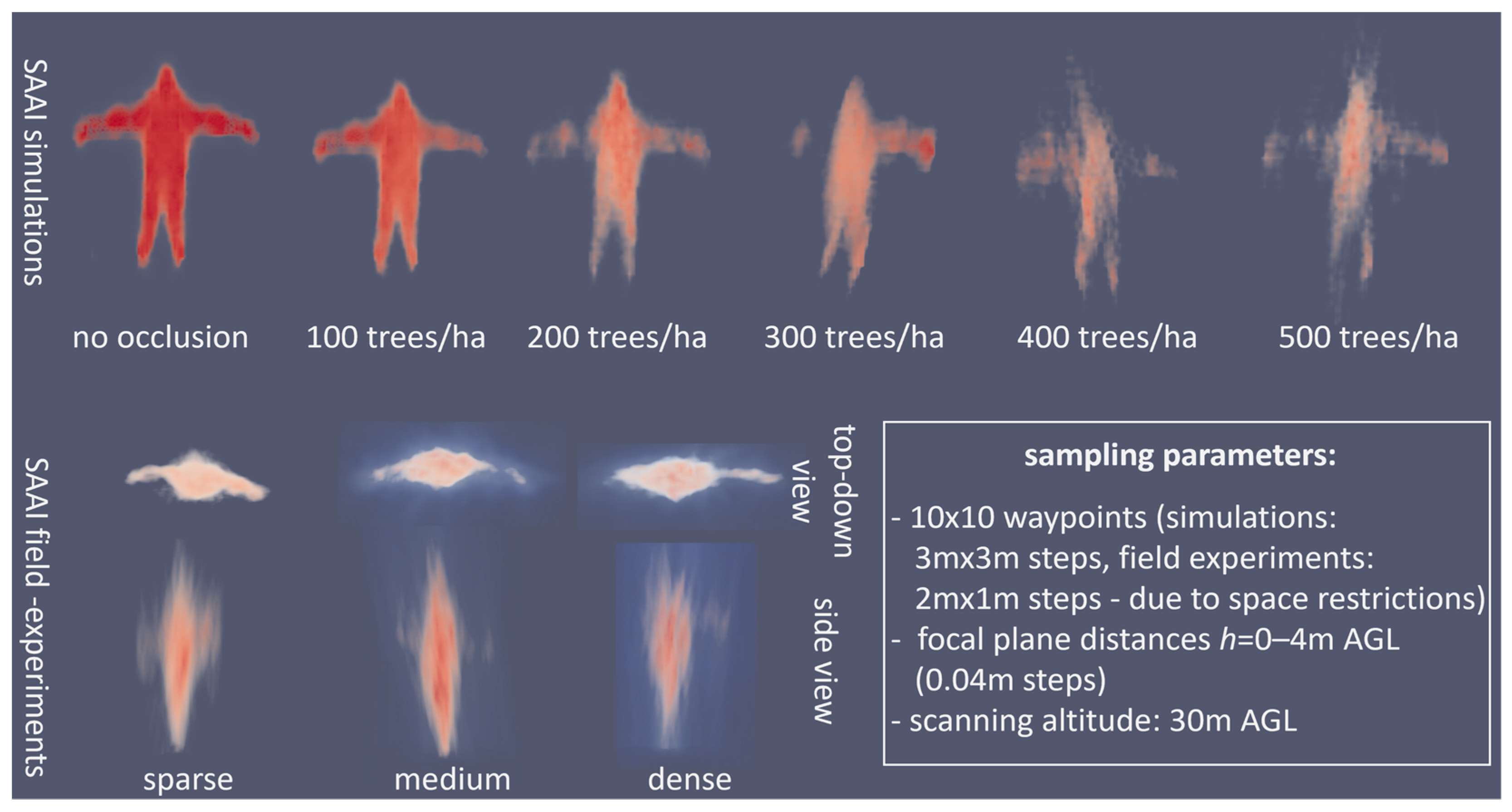
2.1. Simulation

Our simulations were realized with a procedural forest algorithm called ProcTree (https://github.com/supereggbert/proctree.js, accessed on 30 August 2023) and was implemented using WebGL. We computed 512 × 512 px aerial images (color-mapped thermal images) for drone flights over a predefined area using defined sampling parameters (e.g., waypoints, altitudes, and camera fields-of-view). Figure 1 shows examples of such simulated images. The virtual rendering camera (FOV = 50 deg in our case) applied perspective projection and was aligned with its look-at vector orthogonal to the ground surface normal (i.e., pointing downwards). Procedural tree parameters, such as tree height (20–25 m), trunk length (4–8 m), trunk radius (20–50 cm), and leaf size (5–20 cm), were used to generate a representative mixture of tree species. Finally, a seeded random generator was applied to generate a variety of trees at defined densities and degrees of similarity. Besides the thermal effects of direct sunlight on the tree crowns, other environmental properties, such as varying tree species, foliage, and time of year, were assumed to be constant. The simulated forest densities were considered sparse with 300 trees/ha, medium with 400 trees/ha, and dense with 500 trees/ha. The simulated environment was a 1 ha procedural forest with one hidden avatar lying on the ground. Since the maximal visibility of the target (i.e., the maximal pixel coverage of the target’s projected footprint in the simulated images under no occlusion) is known, the simulation allows for quantitative comparisons in target visibility and precision, as presented in Section 3.

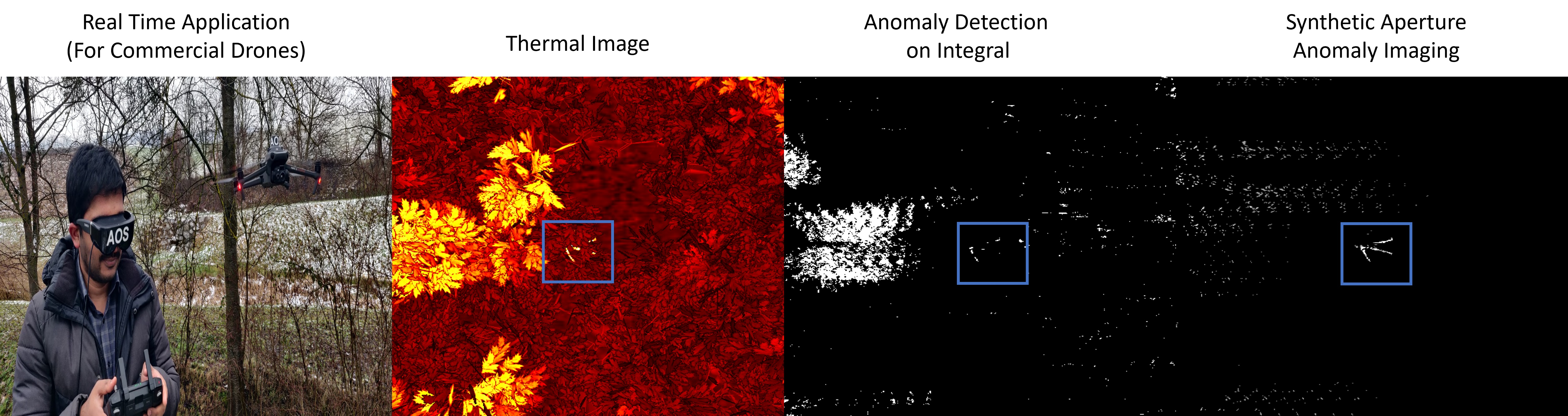
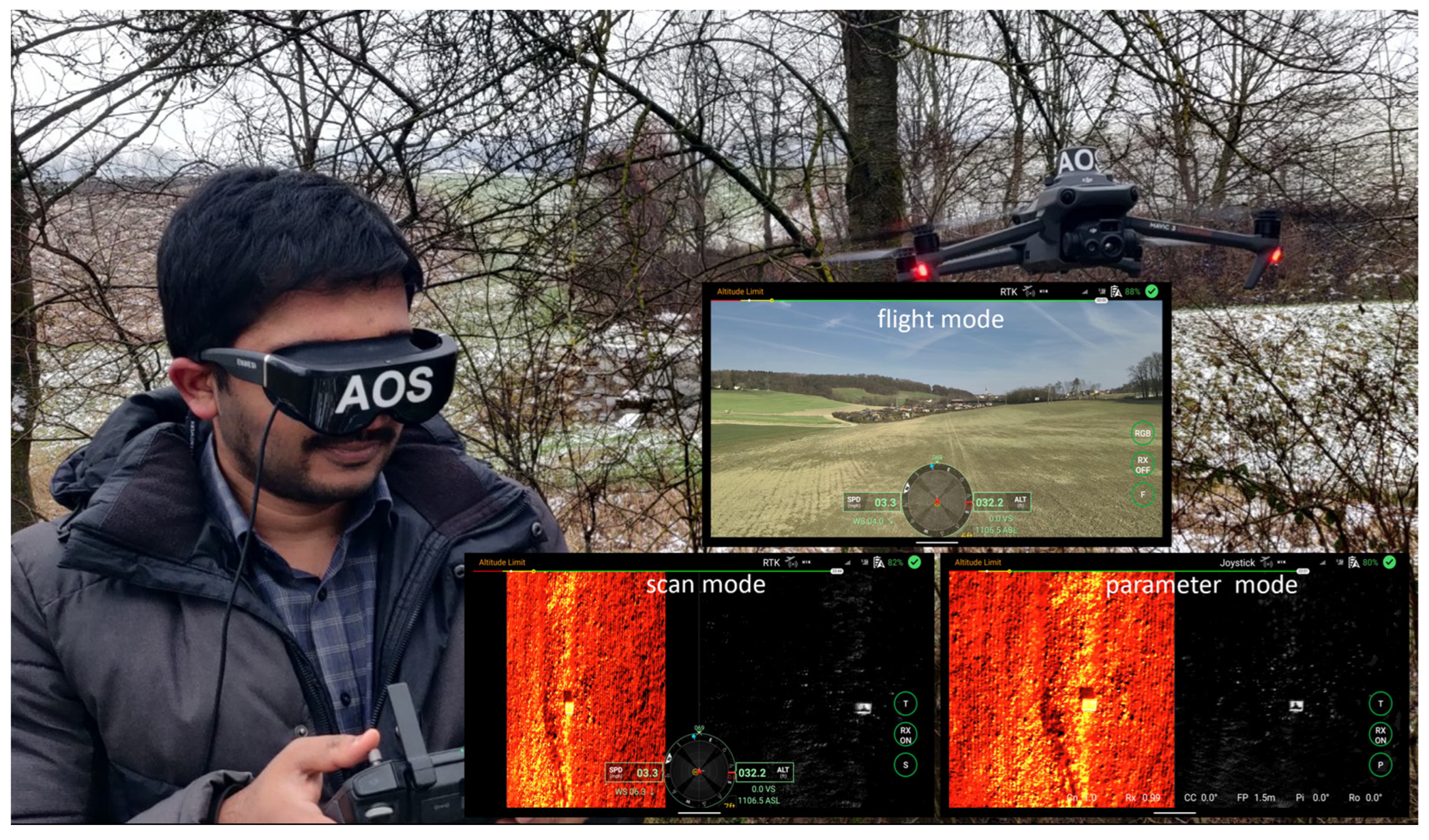
2.2. Real-Time Application on Commercial Drones
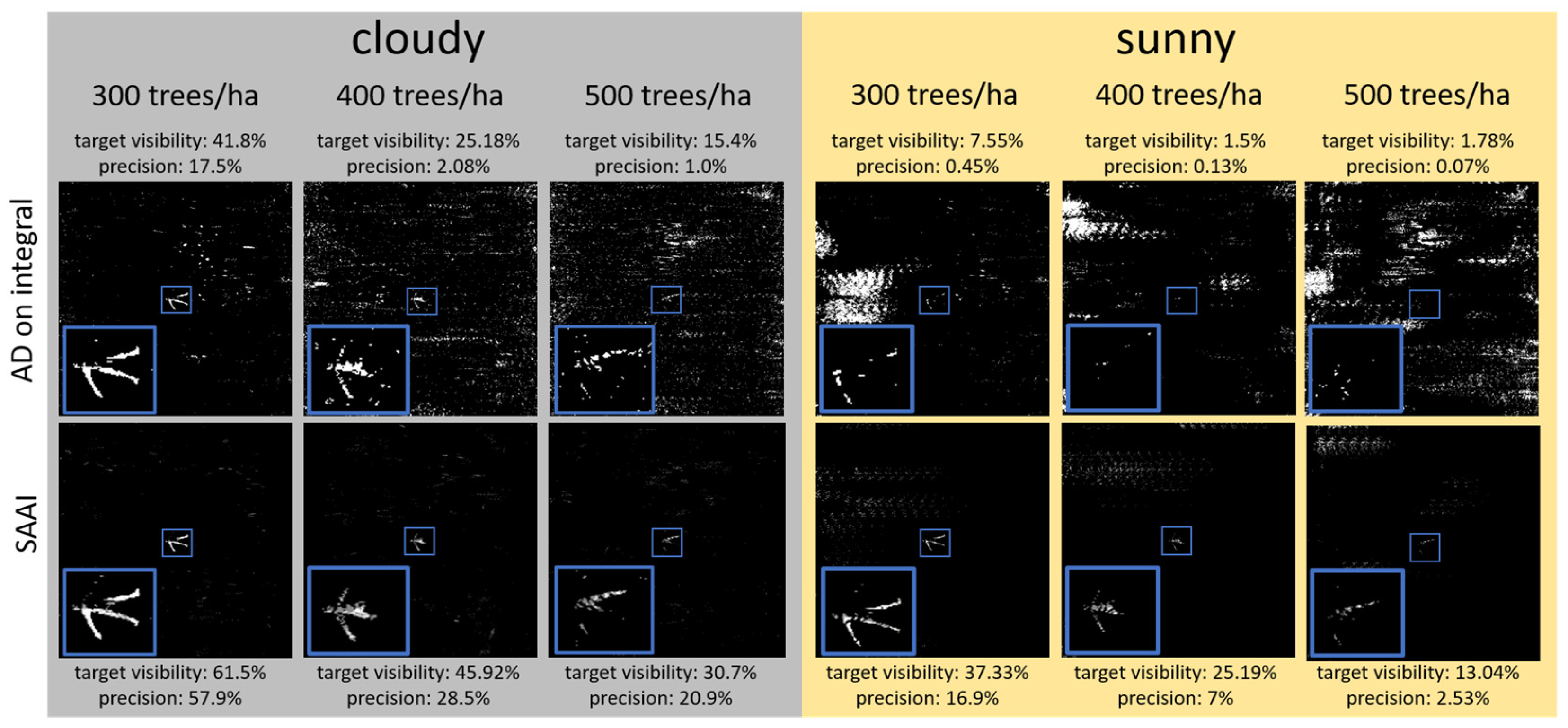
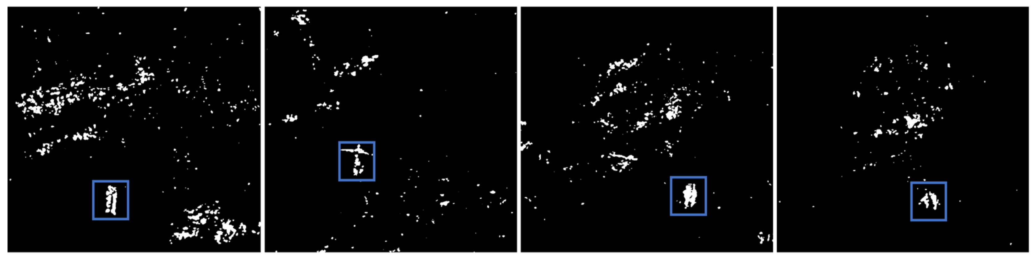
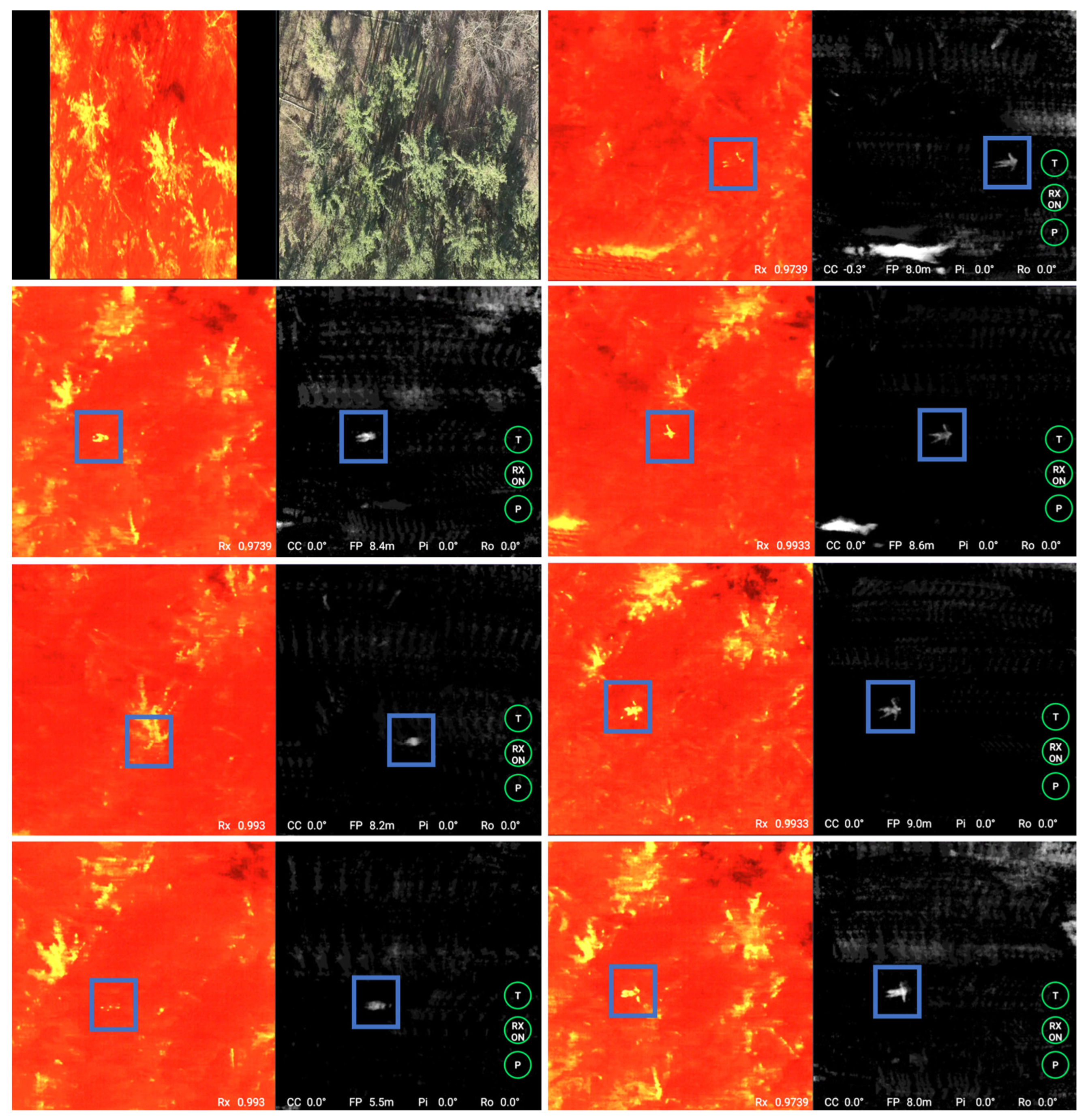
The real-time application used for our field experiments was developed using DJI’s Mobile SDK 5, which currently supports the new DJI enterprise series, such as Mavic 3T and Matric 30T. For the results of the field experiments presented in Section 3, we applied a DJI Mavic 3T with a 640 × 512@30 Hz thermal camera (61 deg FOV, f/1.0, 5 m-infinity focus) at an altitude of 35 m AGL. The application is executed on the Android 10 smart controllers (DJI RC Plus and Pro) and, as shown in Figure 3, supports three modes of operation: a flight mode that displays the live video stream of either the wide FOV, thermal, or zoom RGB camera, and a scan mode and parameter mode, in which single aerial images are recorded and integrated, the visualization parameters are interactively adjusted, and the live video stream (RGB or thermal) is displayed on the left side, while the resulting integral image (thermal, RGB, or RX = SAAI/AD on integral image) is shown on the right side. The application supports networked Real-Time Kinematics (RTK), if available. The application, including details on installation and operation, is freely available (https://github.com/JKU-ICG/AOS/ accessed on 30 August 2023).
Figure 4 illustrates a schematic overview of the application’s main software system components. It consists of three parallelly running threads that share images and telemetry data through queues. This is essential for buffering slight temporal differences in the runtime of these threads. The first thread (implemented in Java) receives raw (RGB or thermal) video and telemetry data (RTK corrected GPS, compass direction, and gimbal angles) from the drone, decodes the video data, and selects frames (video-telemetry pairs) based on the defined sampling distance. Thus, if the selected sampling distance is 0.5 m, for example, only frames at a flight distance of 0.5 m are selected and pushed into the queue. Note that, while video streams are delivered at 30 Hz, GPS sampling is limited to a maximum of 10 Hz (10 Hz with RTK, 5 Hz with conventional GPS). Therefore, SAAI results are displayed at a speed of 10 Hz/5 Hz. The next thread (implemented in PyTorch for C++) computes a single image RX detection on the GPU of the smart controller. It receives the preselected frames from the first queue and computes the per-pixel anomalies based on the selected RX threshold t (which is called Rx in the application’s GUI). These frames are then forwarded through the second queue to the third thread. The last thread (implemented in C++) registers a window of images (i.e., the n latest frames, where n is the integral window size of the SA). This registration is performed based on telemetry data and the provided visualization parameters, as described in Table 1.
The final integral image is displayed on the right side of the split screen. Note that FP, Ro, Pi, CC, Cn, and Rx can be interactively changed in parameter mode, as explained above. The sampling distance and integral window size are defined in the application’s settings. Note that sampling distance times integral window size equals the SA size (a in Figure 1).
Performance measures were timed on a DJI RC Pro Enterprise running on Android 10: the initial thread required 10–20 ms, the second thread required 5–10 ms, and the last thread took approximately 40 ms. Overall, this led to approximately a 45–75 ms processing time. However, the maximum GPS sampling speed of 10 Hz (RTK) defers the processing time to 100 ms in practice.

3. Results

The results presented in Figure 5 are based on simulations conducted as described in Section 2.1, using procedural forests of different densities (300–500 trees/ha) with a hidden avatar lying on the ground. The far-infrared (thermal) channel is computed for cloudy and sunny environmental conditions, and is color-mapped (hot color bar, as shown in Figure 2). We compare two cases: First, the thermal channel is integrated, and the RX detector is applied to the integral image (AD on integral image), as performed in [13]. Second, the RX detector is applied to the single images and the resulting anomalies are then integrated (SAAI).
Since the ground truth projection of the unoccluded target can be computed in the simulation, its maximum visibility without occlusion is known. This is the area of the target’s projected footprint in the simulated images. One quality metric that can be considered is the remaining target visibility in case of occlusion. Thus, a target visibility of 61.5%, for instance, indicates that 61.5% of the complete target’s footprint is still visible in presence of occlusion. However, target visibility considers only true positives (i.e., if a pixel that belongs to the target is visible or not). To consider false positives as well (i.e., pixels that are indicated abnormal but do not belong to the target), we use precision as a second metric, which is the intensity integral of all true positives divided by the sum of true positives and false positives intensity integrals. High precision values indicate more true positives and fewer false positives.
As shown in Figure 5, integrating anomalies (SAAI) always outperforms anomaly detections on integral images (AD on integral images), both in target visibility and precision. This is the case for all forest densities and also for cloudy and sunny environmental conditions. Target visibility and precision generally drop with higher densities due to more severe occlusion. In particular, under sunny conditions, many and large false positive areas are detected. This is due to the higher thermal radiation of non-target objects, such as on tree-tops, that appear as hot as the target. Under cloudy and cool conditions, the highest thermal radiation is mainly from the target itself.
One major difference between AD on integral images and SAAI is that the first case results in a binary mask, as pixels are being indicated to be abnormal if they belong to the t% of pixels with the highest anomaly scores α (Equation (1)), while for the latter case, the detections of the t% most abnormal pixels of each single image are integrated. This leads to a non-binary value per pixel, which corresponds to visibility (i.e., how often an abnormal point on the focal plane was captured free of occlusion).
Note that, because the background models of single and integral images differ significantly [13], two different RX thresholds had to be applied to compare the two cases in Figure 5 (t = 99% for AD on integral images, and t = 90% for SAAI). They have been chosen such that the results of both cases approach each other as well as possible. For all other thresholds, SAAI outperforms AD on integral images even more. Section 4 discusses in more detail why SAAI outperforms AD on integral images.
Figure 6 illustrates the results of real field experiments (with individual experiment values) under the more difficult (i.e., sunny) conditions for thermal imaging. For these experiments, we implemented real-time SAAI on commercially available drones, as explained in Section 2.2. In contrast to the simulated results, a ground truth does not exist here. Consequently, the results can only be presented and compared visually.
Compared to single thermal aerial images, where the target is partially or fully occluded and its fractional footprint is often indistinguishable from false heat signals in the surrounding area, SAAI clearly reveals the target’s shape and suppresses false heat signals well. Figure 7 shows that applying AD on integral images under the same conditions results in many false detections that form large pixel clusters, just as in our simulations. Identifying the target can be challenging under these conditions.

4. Discussion

It was previously shown that, in the presence of foliage occlusion, anomaly detection performs significantly better in integral images resulting from synthetic aperture imaging than in conventional single aerial images [13]. The reason for this is the much more uniform background statistics of integral images compared to single images. In this article, we demonstrate that integrating detected anomalies (i.e., applying anomaly detection to single aerial images first and then integrating the results) significantly outperforms detecting anomalies in integral images (i.e., integrating single aerial images first and then applying anomaly detection to the result). This leads to enhanced occlusion removal and outlier suppression, and consequently to higher chances for detecting otherwise occluded targets visually (i.e., by a human observer) or computationally (e.g., by an automatic classification method). The RX detector applied in our experiment serves as a proof-of-concept and can be substituted with more advanced anomaly detectors. Nonetheless, we believe that the pronounced effectiveness of integrating detected anomalies over applying anomaly detection to integral images will remain. We achieved an increase in target visibility as well as in precision of an additional 20% on average in our experiments.
This finding can be explained as follows: with respect to Figure 1, the integral signal of a target point F is the sum of all registered ray contributions of all overlapping aerial images. This integral signal consists of a mixture of unoccluded (signal of target) and occluded (signal of forest background) ray contributions. Only if the unoccluded contributions dominate, the resulting integral pixel can robustly be detected as an anomaly. On the one hand, applying anomaly detection before integration zeros out occluding rays initially, while assigning the highest possible signal contribution of one to the target rays. Thus, integrating detected anomalies reduces background noise in the integrated target signal. In fact, the integrated target signal corresponds directly to visibility (i.e., how often an abnormal point on the focal plane was captured free of occlusion). On the other hand, the integral signals of occluders (e.g., O in Figure 1) can also be high (e.g., tree crowns that are headed by sunlight). They would be considered as anomalies if they differ too much from the background model and would be binary masked just like the targets. Consequently, anomaly detection applied to integral images can lead to severe false positives that are indistinguishable from true positives, as shown in Figure 5 (top row) and Figure 7. Certainly, this is also the case when anomaly detection is applied to single images. But integrating the anomaly masks suppresses the contribution of false positives, as their rays are not registered on the focal plane, as shown in Figure 5 (bottom row) and Figure 6. Only the false positives located directly on the focal plane (e.g., open ground patches that are heated by sunlight, as the large bright patches shown by the two top-right examples in Figure 6) remain registered and can lead to classification confusion. For dense forests, however, we can expect that large open ground patches are rare, and that most of the sunlight that could cause false detections is reflected by the tree crowns.

5. Conclusions and Future Work

Reliable visual and automatic target detection is essential for many drone-based applications encompassing search and rescue operations, early wildfire detection, wildlife observation, border control, and surveillance. Nonetheless, the persistent challenge of substantial occlusion remains a critical concern that can be addressed through occlusion removal techniques, such as the one presented in this article.
Derived from our experimental findings performed under different environmental conditions and varying forest densities, the precision range for Anomaly Detection applied to integral images (AD on integral images) spans from 0.07% to 17.5%, whereas in the case of Synthetic Aperture Anomaly Imaging (SAAI) it extends from 2.53% to 57.9%. Similarly, our experiments reveal that the minimum and maximum target visibility for AD on integral images are 1.5% and 41.8%, respectively. Here, SAAI leads to superior results of 13.04% and 61.5%, respectively. Overall, SAAI achieves an average enhancement of 20% over AD on integral images in both target visibility and precision through our experiments.
Our previous investigations have shown that the utilization of additional channels, such as the fusion of RGB and thermal data (instead of relying solely on RGB or thermal data), yields a significant enhancement in anomaly detection [16]. Therefore, our future work will involve extending anomaly detection to incorporate even more channels—including optical flow. In line with this, we will be conducting in-depth studies of anomalies triggered by motion patterns. Together with synthetic aperture sensing, this holds the potential of amplifying the signal of strongly occluded moving targets.
Moreover, we are actively exploring the integration of advanced deep-learning classification methods [11] and believe that applying classification to the results derived from SAAI will yield a superior performance compared to its application to conventional integral images. This enhancement should result from the initial suppression of false positive pixels by SAAI.
Using the same scanned single images, SAAI can easily be extended to 3D volume integration by simply repeating the 2D anomaly image integration process, as explained in Section 1, for different focal plane distances (h). This results in a volumetric focal stack of integrated anomalies at each volumetric position in space, as shown with initial results from simulations and field experiments in Figure 8. However, whether target classification in 3D is more efficient than in 2D needs to be explored.
As we progress, our objective is to leverage these findings to continually elevate the efficacy of target detection within the realm of aerial imaging.

Supplementary Materials

Supporting information and the AOS application for DJI can be downloaded at: https://github.com/JKU-ICG/AOS/ (AOS for DJI), accessed on 30 August 2023. The supplementary video is available at: https://user-images.githubusercontent.com/83944465/217470172-74a2b272-2cd4-431c-9e21-b91938a340f2.mp4, accessed on 30 August 2023.

Author Contributions

Conceptualization, O.B.; methodology, O.B. and R.J.A.A.N.; software R.J.A.A.N.; validation, R.J.A.A.N. and O.B.; formal analysis, R.J.A.A.N. and O.B.; investigation, R.J.A.A.N.; resources, R.J.A.A.N.; data curation, R.J.A.A.N.; writing—original draft preparation, O.B.; writing—review and editing, O.B. and R.J.A.A.N.; visualization, O.B. and R.J.A.A.N.; supervision, O.B.; project administration, O.B.; funding acquisition, O.B. All authors have read and agreed to the published version of the manuscript.

Funding

This research was funded by the Austrian Science Fund (FWF) and German Research Foundation (DFG) under grant numbers P 32185-NBL and I 6046-N, and by the State of Upper Austria and the Austrian Federal Ministry of Education, Science and Research via the LIT–Linz Institute of Technology under grant number LIT-2019-8-SEE-114. Open Access Funding by the Austrian Science Fund (FWF).

Data Availability Statement

All experimental data presented in this article are available at: https://doi.org/10.5281/zenodo.7867080, accessed on 30 August 2023.

Acknowledgments

We thank Francis Seits, Rudolf Ortner, and Indrajit Kurmi for contributing to the implementation of the application, and Mohammed Abbass for supporting the field experiments.

Conflicts of Interest

The authors declare no conflict of interest.

References

  1. Indrajit, K.; Schedl, D.C.; Bimber, O. Airborne Optical Sectioning. J. Imaging 2018, 4, 102. [Google Scholar] [CrossRef]
  2. Oliver, B.; Kurmi, I.; Schedl, D.C. Synthetic aperture imaging with drones. IEEE Comput. Graph. Appl. 2019, 39, 8–15. [Google Scholar] [CrossRef]
  3. Indrajit, K.; Schedl, D.C.; Bimber, O. A statistical view on synthetic aperture imaging for occlusion removal. IEEE Sens. J. 2019, 19, 9374–9383. [Google Scholar] [CrossRef]
  4. Indrajit, K.; Schedl, D.C.; Bimber, O. Thermal airborne optical sectioning. Remote Sens. 2019, 11, 1668. [Google Scholar] [CrossRef]
  5. Indrajit, K.; Schedl, D.C.; Bimber, O. Fast automatic visibility optimization for thermal synthetic aperture visualization. IEEE Geosci. Remote Sens. Lett. 2020, 18, 836–840. [Google Scholar] [CrossRef]
  6. Indrajit, K.; Schedl, D.C.; Bimber, O. Pose error reduction for focus enhancement in thermal synthetic aperture visualization. IEEE Geosci. Remote Sens. Lett. 2021, 19, 1–5. [Google Scholar] [CrossRef]
  7. Seits, F.; Kurmi, I.; Nathan, R.J.A.A.; Ortner, R.; Bimber, O. On the Role of Field of View for Occlusion Removal with Airborne Optical Sectioning. arXiv 2022, arXiv:2204.13371. [Google Scholar]
  8. David, C.S.; Kurmi, I.; Bimber, O. Airborne optical sectioning for nesting observation. Sci. Rep. 2020, 10, 7254. [Google Scholar] [CrossRef]
  9. David, C.S.; Kurmi, I.; Bimber, O. Search and rescue with airborne optical sectioning. Nat. Mach. Intell. 2020, 2, 783–790. [Google Scholar] [CrossRef]
  10. David, C.S.; Kurmi, I.; Bimber, O. An autonomous drone for search and rescue in forests using airborne optical sectioning. Sci. Robot. 2021, 6, eabg1188. [Google Scholar] [CrossRef]
  11. Indrajit, K.; Schedl, D.C.; Bimber, O. Combined person classification with airborne optical sectioning. Sci. Rep. 2022, 12, 3804. [Google Scholar] [CrossRef]
  12. Rudolf, O.; Kurmi, I.; Bimber, O. Acceleration-Aware Path Planning with Waypoints. Drones 2021, 5, 143. [Google Scholar] [CrossRef]
  13. Nathan, R.J.A.A.; Kurmi, I.; Schedl, D.C.; Bimber, O. Through-Foliage Tracking with Airborne Optical Sectioning. J. Remote Sens. 2022, 2022, 9812765. [Google Scholar] [CrossRef]
  14. Nathan, A.A.; John, R.; Kurmi, I.; Bimber, O. Inverse Airborne Optical Sectioning. Drones 2022, 6, 231. [Google Scholar] [CrossRef]
  15. Nathan, A.A.; John, R.; Kurmi, I.; Bimber, O. Drone swarm strategy for the detection and tracking of occluded targets in complex environments. Nat. Commun. Eng. 2023, 2, 55. [Google Scholar] [CrossRef]
  16. Francis, S.; Kurmi, I.; Bimber, O. Evaluation of Color Anomaly Detection in Multispectral Images for Synthetic Aperture Sensing. Eng 2022, 3, 541–553. [Google Scholar] [CrossRef]
  17. Moreira, A.; Prats-Iraola, P.; Younis, M.; Krieger, G.; Hajnsek, I.; Papathanassiou, K.P. A tutorial on synthetic aperture radar. IEEE Geosci. Remote Sens. Mag. 2013, 1, 6–43. [Google Scholar] [CrossRef]
  18. Wiley Carl, A. Pulsed Doppler Radar Methods and Apparatus. U.S. Patent No. 3,196,436, 20 July 1965. [Google Scholar]
  19. Cutrona, L.; Vivian, W.; Leith, E.; Hall, G. Synthetic aperture radars: A paradigm for technology evolution. IRE Trans. Mil. Electron 1961, 127–131. [Google Scholar] [CrossRef]
  20. Farquharson, G.; Woods, W.; Stringham, C.; Sankarambadi, N.; Riggi, L. The capella synthetic aperture radar constellation. In Proceedings of the EUSAR 2018 12th European Conference on Synthetic Aperture Radar, Aachen, Germany, 4–7 June 2018; VDE: Bavaria, Germany, 2018. [Google Scholar]
  21. Fulong, C.; Lasaponara, R.; Masini, N. An overview of satellite synthetic aperture radar remote sensing in archaeology: From site detection to monitoring. J. Cult. Herit. 2017, 23, 5–11. [Google Scholar] [CrossRef]
  22. Zhang, Z.; Lin, H.; Wang, M.; Liu, X.; Chen, Q.; Wang, C.; Zhang, H. A Review of Satellite Synthetic Aperture Radar Interferometry Applications in Permafrost Regions: Current Status, Challenges, and Trends. IEEE Geosci. Remote Sens. Mag. 2022, 10, 93–114. [Google Scholar] [CrossRef]
  23. Kumar, R.A.; Parida, B.R. Predicting paddy yield at spatial scale using optical and Synthetic Aperture Radar (SAR) based satellite data in conjunction with field-based Crop Cutting Experiment (CCE) data. Int. J. Remote Sens. 2021, 42, 2046–2071. [Google Scholar] [CrossRef]
  24. Reigber, A.; Scheiber, R.; Jager, M.; Prats-Iraola, P.; Hajnsek, I.; Jagdhuber, T.; Papathanassiou, K.P.; Nannini, M.; Aguilera, E.; Baumgartner, S.; et al. Very-high-resolution airborne synthetic aperture radar imaging: Signal processing and applications. Proc. IEEE 2012, 101, 759–783. [Google Scholar] [CrossRef]
  25. Sumantyo, J.T.S.; Chua, M.Y.; Santosa, C.E.; Panggabean, G.F.; Watanabe, T.; Setiadi, B.; Sumantyo, F.D.S.; Tsushima, K.; Sasmita, K.; Mardiyanto, A.; et al. Airborne circularly polarized synthetic aperture radar. IEEE J. Sel. Top. Appl. Earth Obs. Remote Sens. 2020, 14, 1676–1692. [Google Scholar] [CrossRef]
  26. Tsunoda, S.I.; Pace, F.; Stence, J.; Woodring, M.; Hensley, W.H.; Doerry, A.W.; Walker, B.C. Lynx: A high-resolution synthetic aperture radar. In Proceedings of the 2000 IEEE Aerospace Conference, Orlando, FL, USA, 25 March 2000; Proceedings (Cat. No. 00TH8484). Volume 5. [Google Scholar]
  27. Fernandez, M.G.; Lopez, Y.A.; Arboleya, A.A.; Valdes, B.G.; Vaqueiro, Y.R.; Andres, F.L.-H.; Garcia, A.P. Synthetic aperture radar imaging system for landmine detection using a ground penetrating radar on board a unmanned aerial vehicle. IEEE Access 2018, 6, 45100–45112. [Google Scholar] [CrossRef]
  28. Tomonori, D.; Sugiyama, T.; Kishimoto, M. Development of SAR system installable on a drone. In Proceedings of the EUSAR 2021 13th European Conference on Synthetic Aperture Radar, Virtual, 29 March–1 April 2021; VDE: Bavaria, Germany, 2021. [Google Scholar]
  29. Mondini, A.C.; Guzzetti, F.; Chang, K.-T.; Monserrat, O.; Martha, T.R.; Manconi, A. Landslide failures detection and mapping using Synthetic Aperture Radar: Past, present and future. Earth-Sci. Rev. 2021, 216, 103574. [Google Scholar] [CrossRef]
  30. Rosen, P.A.; Hensley, S.; Joughin, I.R.; Li, F.K.; Madsen, S.N.; Rodriguez, E.; Goldstein, R.M. Synthetic aperture radar interferometry. Proc. IEEE 2000, 88, 333–382. [Google Scholar] [CrossRef]
  31. Prickett, M.J.; Chen, C.C. Principles of inverse synthetic aperture radar/ISAR/imaging. In Proceedings of the EASCON’80, Electronics and Aerospace Systems Conference, Arlington, VA, USA, September 29–1 October 1980. [Google Scholar]
  32. Risto, V.; Neuberger, N. Inverse Synthetic Aperture Radar Imaging: A Historical Perspective and State-of-the-Art Survey. IEEE Access 2021, 9, 113917–113943. [Google Scholar] [CrossRef]
  33. Caner, O. Inverse Synthetic Aperture Radar Imaging with MATLAB Algorithms; John Wiley & Sons: Hoboken, NJ, USA, 2012; Volume 210. [Google Scholar]
  34. Marino, A.; Sanjuan-Ferrer, M.J.; Hajnsek, I.; Ouchi, K. Ship detection with spectral analysis of synthetic aperture radar: A comparison of new and well-known algorithms. Remote Sens. 2015, 7, 5416–5439. [Google Scholar] [CrossRef]
  35. Yong, W.; Chen, X. 3-D interferometric inverse synthetic aperture radar imaging of ship target with complex motion. IEEE Trans. Geosci. Remote Sens. 2018, 56, 3693–3708. [Google Scholar] [CrossRef]
  36. Xu, G.; Zhang, B.; Chen, J.; Wu, F.; Sheng, J.; Hong, W. Sparse Inverse Synthetic Aperture Radar Imaging Using Structured Low-Rank Method. IEEE Trans. Geosci. Remote Sens. 2021, 60, 1–12. [Google Scholar] [CrossRef]
  37. Fabrizio, B.; Corsini, G. Autofocusing of inverse synthetic aperture radar images using contrast optimization. IEEE Trans. Aerosp. Electron. Syst. 1996, 32, 1185–1191. [Google Scholar] [CrossRef]
  38. Bai, X.; Zhou, F.; Xing, M.; Bao, Z. Scaling the 3-D image of spinning space debris via bistatic inverse synthetic aperture radar. IEEE Geosci. Remote Sens. Lett. 2010, 7, 430–434. [Google Scholar] [CrossRef]
  39. Anger, S.; Jirousek, M.; Dill, S.; Peichl, M. Research on advanced space surveillance using the IoSiS radar system. In Proceedings of the EUSAR 2021 13th European Conference on Synthetic Aperture Radar, Online, 29 March 2021; VDE: Bavaria, Germany, 2021. [Google Scholar]
  40. Vossiek, M.; Urban, A.; Max, S.; Gulden, P. Inverse synthetic aperture secondary radar concept for precise wireless positioning. IEEE Trans. Microw. Theory Tech. 2007, 55, 2447–2453. [Google Scholar] [CrossRef]
  41. Shyr-Long, J.; Chieng, W.-H.; Lu, H.-P. Estimating speed using a side-looking single-radar vehicle detector. IEEE Trans. Intell. Transp. Syst. 2013, 15, 607–614. [Google Scholar] [CrossRef]
  42. Ye, X.; Zhang, F.; Yang, Y.; Zhu, D.; Pan, S. Photonics-based high-resolution 3D inverse synthetic aperture radar imaging. IEEE Access 2019, 7, 79503–79509. [Google Scholar] [CrossRef]
  43. Neeraj, P.; Ram, S.S. Classification of automotive targets using inverse synthetic aperture radar images. IEEE Trans. Intell. Veh. 2022, 7, 675–689. [Google Scholar] [CrossRef]
  44. Ronny, L.; Leshem, A. Synthetic aperture radio telescopes. IEEE Signal Process. Mag. 2009, 27, 14–29. [Google Scholar] [CrossRef]
  45. Dainis, D.; Lagadec, T.; Nuñez, P.D. Optical aperture synthesis with electronically connected telescopes. Nat. Commun. 2015, 6, 6852. [Google Scholar] [CrossRef]
  46. Ralston, T.S.; Marks, D.L.; Carney, P.S.; Boppart, S.A. Interferometric synthetic aperture microscopy. Nat. Phys. 2007, 3, 129–134. [Google Scholar] [CrossRef]
  47. Roy, E. Introduction to Synthetic Aperture Sonar. Sonar Syst. 2011, 1–11. [Google Scholar] [CrossRef]
  48. Hayes Michael, P.; Peter, T. Gough. Synthetic aperture sonar: A review of current status. IEEE J. Ocean. Eng. 2009, 34, 207–224. [Google Scholar] [CrossRef]
  49. Hansen, R.E.; Callow, H.J.; Sabo, T.O.; Synnes, S.A.V. Challenges in seafloor imaging and mapping with synthetic aperture sonar. IEEE Trans. Geosci. Remote Sens. 2011, 49, 3677–3687. [Google Scholar] [CrossRef]
  50. Heiko, B.; Birk, A. Synthetic aperture sonar (SAS) without navigation: Scan registration as basis for near field synthetic imaging in 2D. Sensors 2020, 20, 4440. [Google Scholar] [CrossRef]
  51. Jensen, J.A.; Nikolov, S.I.; Gammelmark, K.L.; Pedersen, M.H. Synthetic aperture ultrasound imaging. Ultrasonics 2006, 44, e5–e15. [Google Scholar] [CrossRef] [PubMed]
  52. Zhang, H.K.; Cheng, A.; Bottenus, N.; Guo, X.; Trahey, G.E.; Boctor, E.M. Synthetic tracked aperture ultrasound imaging: Design, simulation, and experimental evaluation. J. Med. Imaging 2016, 3, 027001. [Google Scholar] [CrossRef]
  53. Zeb, W.B.; Dahl, J.R. Synthetic aperture ladar imaging demonstrations and information at very low return levels. Appl. Opt. 2014, 53, 5531–5537. [Google Scholar] [CrossRef]
  54. Terroux, M.; Bergeron, A.; Turbide, S.; Marchese, L. Synthetic aperture lidar as a future tool for earth observation. In Proceedings of the International Conference on Space Optics—ICSO 2014, Tenerife, Spain, 6–10 October 2014; SPIE: Bellingham, WA, USA, 2017; Volume 10563. [Google Scholar]
  55. Vaish, V.; Wilburn, B.; Joshi, N.; Levoy, M. Using plane + parallax for calibrating dense camera arrays. In Proceedings of the 2004 IEEE Computer Society Conference on Computer Vision and Pattern Recognition, 2004. CVPR 2004, Washington, DC, USA, 27 June–2 July 2004; Volume 1. [Google Scholar]
  56. Vaish, V.; Levoy, M.; Szeliski, R.; Zitnick, C.L.; Kang, S.B. Reconstructing occluded surfaces using synthetic apertures: Stereo, focus and robust measures. In Proceedings of the 2006 IEEE Computer Society Conference on Computer Vision and Pattern Recognition (CVPR’06), New York, NY, USA, 17–22 June 2006; Volume 2. [Google Scholar]
  57. Heng, Z.; Jin, X.; Dai, Q. Synthetic aperture based on plenoptic camera for seeing through occlusions. In Proceedings of the Pacific Rim Conference on Multimedia, Hefei, China, 21–22 September 2018; Springer: Cham, Germany, 2018. [Google Scholar]
  58. Yang, T.; Ma, W.; Wang, S.; Li, J.; Yu, J.; Zhang, Y. Kinect based real-time synthetic aperture imaging through occlusion. Multimed. Tools Appl. 2016, 75, 6925–6943. [Google Scholar] [CrossRef]
  59. Joshi, N.; Avidan, S.; Matusik, W.; Kriegman, D.J. Synthetic aperture tracking: Tracking through occlusions. In Proceedings of the 2007 IEEE 11th International Conference on Computer Vision, Rio de Janeiro, Brazil, 14–20 October 2007. [Google Scholar]
  60. Pei, Z.; Li, Y.; Ma, M.; Li, J.; Leng, C.; Zhang, X.; Zhang, Y. Occluded-object 3D reconstruction using camera array synthetic aperture imaging. Sensors 2019, 19, 607. [Google Scholar] [CrossRef]
  61. Yang, T.; Zhang, Y.; Yu, J.; Li, J.; Ma, W.; Tong, X.; Yu, R.; Ran, L. All-in-focus synthetic aperture imaging. In European Conference on Computer Vision; Springer: Cham, Switzerland, 2014. [Google Scholar]
  62. Pei, Z.; Zhang, Y.; Chen, X.; Yang, Y.-H. Synthetic aperture imaging using pixel labeling via energy minimization. Pattern Recognit. 2013, 46, 174–187. [Google Scholar] [CrossRef]
  63. Reed, I.S.; Yu, X. Adaptive Multiple-Band CFAR Detection of an Optical Pattern with Unknown Spectral Distribution. IEEE Trans. Acoust. Speech Signal Process. 1990, 38, 1760–1770. [Google Scholar] [CrossRef]
  64. Chang, C.-I.; Chiang, S.-S. Anomaly Detection and Classification for Hyperspectral Imagery. IEEE Trans. Geosci. Remote Sens. 2020, 40, 1314–1325. [Google Scholar] [CrossRef]
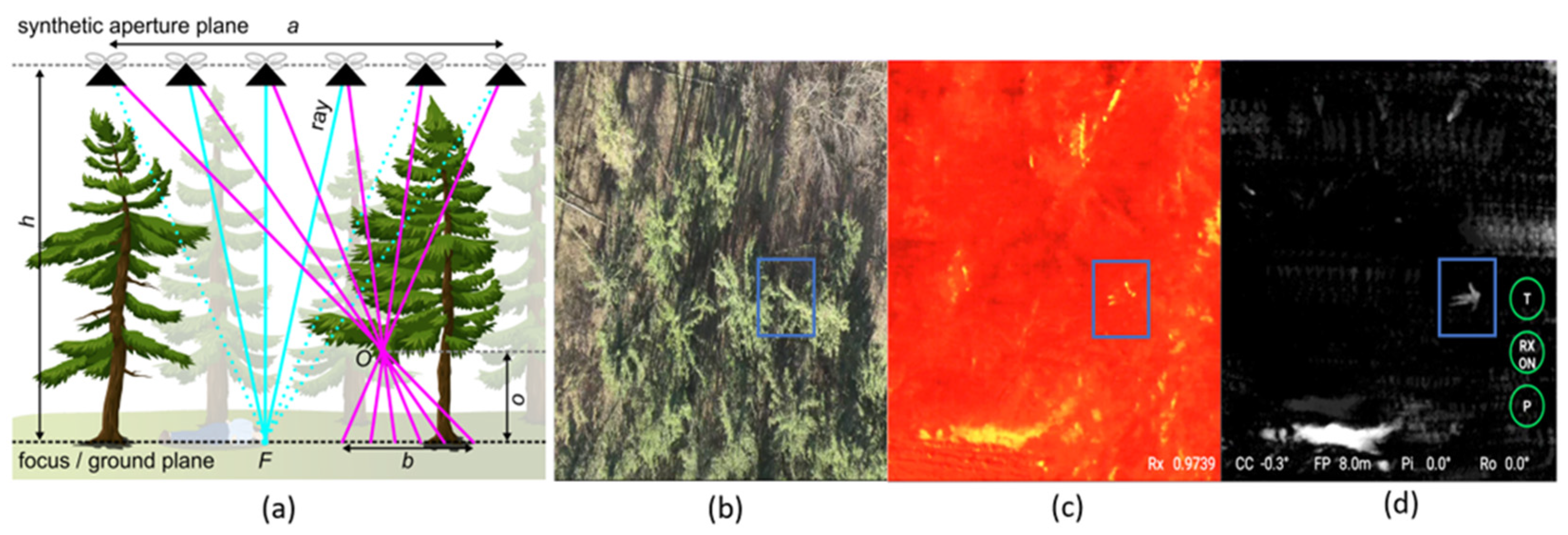
Figure 1. AOS principle (a): registering and integrating multiple images captured along a synthetic aperture of size a while computationally focusing on focal plane F at distance h will defocus occluders O at distance o from F (with a point-spread of b) while focusing targets on F. Conventional RGB (b) and color-mapped thermal (c) aerial images of forest with occluded person [blue box] on the ground. Suppressed occlusion when integrating detected anomalies from 30 thermal images captured along a synthetic aperture of a = 15 m at h = 35 m AGL (d).
Remotesensing 15 04369 g001
Figure 2. Top row: integrating single aerial images (simulated, color-mapped thermal images in this example) first and applying anomaly detection (AD) on the integral image next. Bottom row: applying anomaly detection to single aerial images first, and then integrating the detected anomalies (SAAI). Results are simulated with a procedural forest model under sunny conditions (see Section 2.1). RX is used for both examples. Detected person and its close-up (blue box).
Remotesensing 15 04369 g002
Figure 3. Our real-time SAAI implementation for DJI enterprise platforms and its common process of operation: (1) Take off and fly to target area in flight mode. (2) Scan in target area by flying a linear sideways path in scan mode. (3) Fine-tune visualization parameters (focal plane, compass correction, contrast, RX threshold) in parameter mode. Steps 2 and 3 can be repeated to cover larger areas. Operation supports interactive visualization directly on the smart control as well as first person view (FPV) using additional goggles.
Remotesensing 15 04369 g003
Figure 4. Software system overview: The main components of our application are three parallel running threads that exchange video and telemetry data through two queues. They are distributed on the CPU and GPU of the smart controller for optimal performance and parallel processing.
Remotesensing 15 04369 g004
Figure 5. Simulated results for cloudy (left) and sunny (right) conditions and various forest densities (300, 400, 500 trees/ha): anomaly detection applied to integral images, AD (top row), vs. integrated anomalies, SAAI (bottom row). As in Figure 2, color-mapped thermal images and RX detection were applied for all cases. We use a constant SA of a = 10 m (integrating 10 images at 1 m sampling distance captured from an altitude of h = 35 m AGL). Detected person and its close-up (blue box).
Remotesensing 15 04369 g005
Figure 6. Real SAAI field experiment results under sunny conditions with our application running in real time on the drone’s smart controller: color-mapped single thermal and RGB aerial images of our test site (top left). SAAI detection results for sitting persons (left column) and for persons lying down (right column). The left side of the split screen shows single aerial images (color-mapped thermal) and the right side shows the corresponding SAAI result. See supplementary video for run-time details. We applied a maximal SA of a = 15 m (integrating no more than 30 images at 0.5 m sampling distance, captured from an altitude of h = 35 m AGL). Note that, depending on the local occlusion situations, the target became clearly visible after covering the max. SA to a shorter or larger extent. The RX threshold was individually optimized to achieve the best possible tradeoff between false and true positives (t = 97.4–99.3%). Detected person (blue box).
Remotesensing 15 04369 g006
Figure 7. Real AD on integral image field experiment results (under same conditions as in Figure 4): Here, the RX detector is applied to the thermal integral images, as in [13]. Results show persons lying down (left two images) and sitting persons (right two images). As in Figure 4, the RX threshold was individually optimized to achieve the best possible tradeoff between false and true positives (t = 99.0–99.9%). Detected person (blue box).
Remotesensing 15 04369 g007
Figure 8. SAAI applied to 3D volumes. Results of simulations (top row) and field experiments (bottom row) for different forest densities. Note that, for field experiments, forest density can only be estimated, and that (in contrast to simulations) GPS errors lead to misregistration of integral images—and consequently to additional reconstruction artifacts. For both cases (simulations and field experiments), a 10 × 10 waypoint grid was sampled at 30 m AGL, focal stacks of 100 slices were computed, and the target was a standing person with stretched out arms. Note also that, due to the top-down sampling nature of AOS, the resolution in the axial direction (vertical direction, height) is less than the resolution in spatial directions (horizontal plane). Visibilities are color coded (darker red = higher visibility).
Remotesensing 15 04369 g008
Table 1. Description of visualization parameters (individual experiment values are presented in the results section).
ParameterDescription
(FP)Focal plane distance h
(Pi)Focal plane pitch correction value
(Ro)Focal plane roll correction value
(CC)Compass correction value
(Cn)Contrast enhancement factor
(Rx)Rx threshold
Disclaimer/Publisher’s Note: The statements, opinions and data contained in all publications are solely those of the individual author(s) and contributor(s) and not of MDPI and/or the editor(s). MDPI and/or the editor(s) disclaim responsibility for any injury to people or property resulting from any ideas, methods, instructions or products referred to in the content.

