Abstract
Ship detection technology has achieved significant progress recently. However, for practical applications, lightweight ship detection still remains a very challenging problem since small ships have small relative scales in wide images and are easily missed in the background. To promote the research and application of small-ship detection, we propose a new remote sensing image dataset (VRS-SD v2) and provide a fog simulation method that reflects the actual background in remote sensing ship detection. The experiment results show that the proposed fog simulation is beneficial in improving the robustness of the model for extreme weather. Further, we propose a lightweight detector (LMSD-Net) for ship detection. Ablation experiments indicate the improved ELA-C3 module can efficiently extract features and improve the detection accuracy, and the proposed WGC-PANet can reduce the model parameters and computation complexity to ensure a lightweight nature. In addition, we add a Contextual Transformer (CoT) block to improve the localization accuracy and propose an improved localization loss specialized for tiny-ship prediction. Finally, the overall performance experiments demonstrate that LMSD-Net is competitive in lightweight ship detection among the SOTA models. The overall performance achieves 81.3% in AP@50 and could meet the lightweight and real-time detection requirements.
1. Introduction
Ship detection has gained much attention in the field of marine remote sensing. It has been widely used in sea area management, maritime intelligent traffic, and military target reconnaissance [1,2,3,4]. In sea area management, ship detection can improve sea area security, such as assisting in combating illegal smuggling, illegal oil dumping, and illegal fishing [5,6]. Both maritime intelligent traffic and military target reconnaissance rely on Automatic Identification System (AIS) and Vessel Traffic System (VTS) to determine the current position of a ship. Although AIS and VTS integrate multiple technologies such as Very High Frequency (VHF), Global Positioning System (GPS), and Electronic Chart Display and Information System (ECDIS) technologies, an essential prerequisite is that the ship must be equipped with the corresponding transponder. However, ships below the standard tonnage specified by the International Maritime Organization (IMO) can be unnecessarily equipped with AIS or VTS, which means the Electronic Charts and GPS will not work. In addition to tonnage restrictions, some other special-purpose ships often deliberately turn off their transceivers to avoid radar detection. Therefore, optical image-based remote sensing detection techniques can provide an effective means in these cases. In addition, lightweight research for detection is essential to improve efficiency further.
In recent years, a large number of high-resolution optical remote sensing images (ORSI) have been collected for ship detection since the optimization of optical sensors and accurate geometric correction. However, the following challenges remain in ORSI for ship detection:
Large field of view: Due to different parameter settings of imaging sensors and changes in the flight altitude of the acquisition platform, the target scale changes sharply, which increases the model burden. In addition, the objects of interest in nearshore remote sensing images are usually tiny and densely clustered. Rapid low-altitude flight causes motion blur in dense target areas, posing challenges for detection.
Background interference: In high-resolution images, some environmental conditions, such as fog and low light, will indirectly amplify the interference of sea clutter, wake waves, islands, and other false alarms in the detection. Therefore, it is necessary to consider the impact of complex weather conditions on the image.
Application limitations: Some embedded processors have limited computational performance and storage space. Reducing the computation and spatial complexity of the model with guaranteed performance is crucial for lightweight deployment.
To solve the above problems, traditional methods based on supervised learning are highly dependent on feature descriptors, such as HOG [7], DPM [8], and FourierHOG [9]. For the sparse distribution of small ships on the sea, if feature extraction and calculation are directly implemented within the global sea area, it will greatly increase memory and time consumption. Subsequently, some studies [10,11,12,13] have added a candidate region extraction stage, which could significantly improve the detection speed. However, nearshore dense ships often cause candidate regions to overlap, which is not conducive to feature discrimination. Therefore, these traditional methods are not very robust for unified marine–nearshore ship detection.
With the tremendous success of Convolutional Neural Networks (CNNs) in image classification, CNN has been migrated to object detection frameworks and has played a significant role. Furthermore, the construction of datasets, such as PASCAL VOC challenges [14,15] (VOC2007 and VOC2012), ImageNet large-scale visual recognition challenges [16,17] (ILSVRC2014), and MS-COCO detection challenges [18], has laid a data-driven foundation for the broad application of CNN in object detection.
In the past few decades, two-stage detectors based on CNN have inherited the traditional detection approach, which involves extracting candidate regions first and then discriminating targets, such as SPP-Net [19], R-FCN [20], and Faster R-CNN [21]. Progressively, instead of traditional candidate region extraction methods, related research attempts to use learnable regional proposal networks (RPNs) and achieve state-of-the-art (SOTA) performance in terms of accuracy. For instance, Hu [22] proposed a two-stage detector to improve the accuracy of multi-scale ship targets in complex backgrounds. However, the higher accuracy comes at the cost of detection speed loss. In contrast, single-stage detectors have faster detection velocities, such as RetinaNet [23], Centernet [24], and YOLO series v3–v8 [25,26,27,28,29,30]. For instance, Wang [31] used Yolov4 for ship inspections. Despite a large increase in speed, multi-scale detection performance was poor. For this reason, Ye [32] proposed an adaptive attention fusion mechanism (AAFM) to cope with multi-scale target detection in remote sensing scenes and achieved a better performance. Xu [33] proposed a specific model named LMO-YOLO for ship detection. However, for the detection of small and tiny ship targets, the current accuracy is still low. The low accuracy of these single-stage detectors is the result of sample imbalance. Subsequently, Zhang [34] proposed a balanced learning method to solve the problem of imbalance in the target, scene, and feature pyramid network and classification regression network and achieved better results. In addition, since being inspired by Visual Transformer in Natural Language Processing (NLP), some single-stage detectors have shown great potential, such as Swin Transformer [35,36], Detr [37], and MobileViT [38]. Transformer-based detectors usually use attention matrices to establish the dependencies of sequence elements, which focuses more on contextual information. Remote feature interactions in the transformer can compensate for CNN’s shortcomings. However, high computation complexity and large numbers of parameters are not favorable for deployment. In a word, designing a model should take into account multiple properties such as detection speed, accuracy at multiple scales, and lightweight nature. Therefore, there is still room for improvement to perfect these aspects mentioned above.
With the increasing demand for deployment, lightweight detection has become a necessary evolutionary process. Since the breakthrough of network depth, the vast majority of existing advanced models are pursuing real-time performance and accuracy and have indeed reached a high level. However, to deploy to edge platforms, the detection model must occupy a small amount of memory and participate in less computation. Therefore, some studies have designed model scaling to address different device parameter limitations. For example, Yolov6 [28] has three models with different widths and depths. Two of the three models are used for lightweight deployment. However, one drawback of model scaling is that lightweight models reduce network size while significantly reducing performance. EfficientDet [39] demonstrated in ablation experiments that mixed scaling can reduce the loss of accuracy. In addition, some studies focus on model compression, which minimizes model size as much as possible while ensuring performance. Specifically, SqueezeNext [40] and CondenseNet [41] improved inference speed with parameter pruning and network optimization. The IGC series [42,43,44] pointed out that group convolution could help to reduce the number of parameters. Based on group convolution, ShuffleNetV2 [45] adopted a channel split for feature reusing. While group convolution shares parameters, it still retains redundant features, and parameter sharing affects the accuracy of the prediction box, leading to the missed detection of small targets. It seems to have reached the bottleneck regarding lightweight and performance improvement. Based on the defects mentioned above, there is still room for improvement in designing the detection backbone and shared parameter modes suitable for remote sensing images.
On account of the significant differences in ship scales, it is necessary to design a multi-layer detection model. Most existing layered detection models are based on Feature Pyramid Networks [46] (FPNs). Forming the feature pyramid requires multiple downsamplings and pooling, which may lead to the loss of tiny targets. For example, a small ship with a 12 × 12 dimension has only about one pixel after three layers of pooling, which makes it difficult to distinguish due to its low dimensionality. SSD [47] applied FPN by multiple downsamplings. The receptive field of the underlying feature map is small, which makes it difficult for the network to learn the features of the small targets. Yolov3-spp [25] proposed a spatial pooling pyramid to increase the receptive field of the network, which has a certain improvement in small-target detection. In fact, according to the detection ranking of MS-COCO Challenge1, the detection accuracy of small objects is still far lower than that of large objects. At present, due to differences in resolution, insufficient appearance information, and limited prior knowledge of ORSI, the current technology is still not ideal for detecting tiny ships.
We notice that the expansion of network depth facilitates the mining of higher-level semantic features. High-level semantic features and low-level localization features can reflect the differences of observers well, which brings more potential room to fuse the layered features. For efficient fusion, the layered detection models usually employ bidirectional mapping, including top-down paths and bottom-up paths, such as PANet [48], NAS-FPN [49], BiFPN [39], ASFF [50], and SFAM [51]. Moreover, after feature aggregation, the number of channels of fused features mostly remains consistent with the original features to ensure the width of the network. However, the larger the width of the network, the better it may not necessarily be. Numerous studies have demonstrated an upper limit to network width. When the width reaches a certain scale, the performance will not improve or may even decrease.
We also notice that the design of the detection head is crucial for prediction. The coupled head that is widely used obtains a unified output for localization and classification by sharing convolutional layers between two branches. In contrast, decoupled head designs separate convolutional layers for the localization and classification vectors to obtain more accurate outputs. FCOS [52] pointed out that the decoupled head can speed up model convergence and improve detection accuracy but also brings additional parameters and computational costs. Therefore, the coupled head that shares convolutional layers may be more in line with the lightweight requirement. But how to compensate for the lost performance? With the entry of the transformer into the object detection field, THP-yolov5 [53] treated the transformer as the convolution and utilized the Swin Transformer encoding block [35] to capture the global feature. However, the fully connected layer and residual connections are not optimized enough for the parameters. We urgently need to design a lightweight detection head that combines the advantage of CNN’s inductive bias and the global receptive field capability of ViT, which would improve the detection performance of tiny targets.
As mentioned, although the performance of the above models is impressive, existing frameworks cannot meet the requirements of lightweight and practical remote sensing images. This paper provides an advanced detection model for marine remote sensing applications. The main contributions of this article can be summarized as follows:
- We propose a method to generate fog images in remote sensing datasets to simulate actual background disturbances and compensate for the lack of images with extreme weather. From the perspective of data augmentation and data driven, fog simulation indirectly improves the model’s robustness and detection performance.
- Based on the analysis of the difficulties in optical remote sensing, we have designed a lightweight and layered detection framework (LMSD-Net). Inspired by the detection paradigm of “backbone–neck–head”, in LMSD-Net, an improved module (ELA-C3) is proposed for efficient feature extraction. In the neck, we design a weighted fusion connection (WFC-PANet) to compress the network neck and enhance the representation ability of channel features. In the prediction, we introduce a Contextual Transformer (CoT) to improve the accuracy of dense targets in complex offshore scenes. During the training process, we discovered the degradation problem of CIoU in dealing with small ships and proposed V-CIoU to improve the detection performance of vessels marked by small boxes.
- Based on the VRS ship dataset [54], we added more nearshore images to construct a new ship dataset (VRS-SD v2). The dataset covers different nearshore and offshore scenes, multiple potential disturbances, different target scales, and more dense distributions of tiny ships. Then, we used the proposed fog simulation to process the dataset and obtained the dataset for the actual scenes.
The rest of the paper is organized as follows: Section 2 provides a detailed introduction to the fog simulation and detection framework. In Section 3, we conduct extensive ablation experiments to demonstrate the innovative and efficient framework, and then, we demonstrate the detection results of our model on typical datasets. According to the experiments, Section 4 emphatically discusses the problems solved by the corresponding methods and the experiment results. The final section summarizes the entire paper and briefly discusses future research directions.
2. Methods
An advanced and lightweight ship detection framework consists of three main components: effective data augmentation, efficient feature extraction and fusion, and accurate target prediction. Given the detection difficulties and lightweight requirements mentioned above, these three parts need to be reconsidered. In this section, we have provided a detailed introduction to the methods proposed, including the data augmentation combination and the lightweight detection framework.
2.1. Data Augmentation–Fog Simulation on Actual Remote Sensing Scenes
Whether at sea or near shore, ships are arbitrary in direction and random in distribution. Therefore, we selected several common data augmentation methods, such as cropping, translation, rotation, and random scaling. Then, we adjusted the images’ hue, brightness, and saturation values to address photometric distortion and intensity differences. In addition, we adopted Mosaic [26], which concatenates four images and computes the activation statistics of multiple images together. It has been proven that Mosaic can enrich the detection of backgrounds and improve training efficiency. Essentially, the above data augmentation methods are aimed at achieving more complex representations of the data. Enriched data reduces the gap between the validation, training, and final test sets, so that the network can learn the data distribution better.
In optical remote sensing images, the background of ship targets is often complex and has significant interference with detection. The difficulty of detecting nearshore ships is related to the complex scene of the shore, while the interference of ship detection at sea is mainly caused by islands, wake waves, and sea clutter. Considering more actual scenes, detection work will be carried out under different lighting and weather conditions, especially extreme weather. However, there are few images of existing extreme weather. Due to the absence of cloud and fog scenes in the training and validation sets, the detection performance of the network would be poor. Therefore, simulating the dataset close to the actual scene is necessary to improve the robustness of the model. Thus, we proposed an image degradation method to simulate foggy scenes.
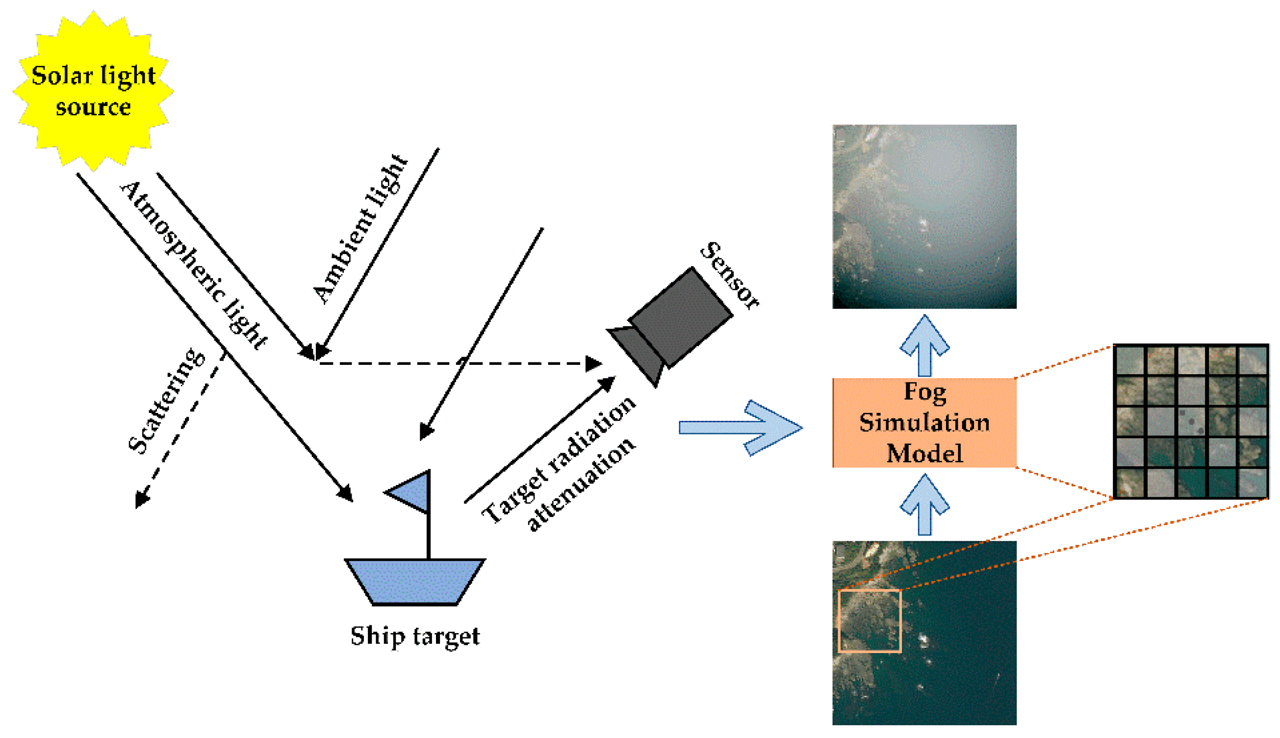
According to the optical model and the imaging mechanism in Figure 1, the influence of fog is modeled as a radiation attenuation function that maps the radiance of a clear scene to the camera sensor. According to the standard optical model, the degradation formula is expressed as follows:
where and represent the original image intensity and observed fog-simulated image intensity at pixel x, respectively, is global atmospheric light, and is the transmission transmittance, which depends on the distance from the lens to the scene and the noise particles in the air. Therefore, the key to simulating fog lies in the estimation of atmospheric light noise and transmission transmittance.
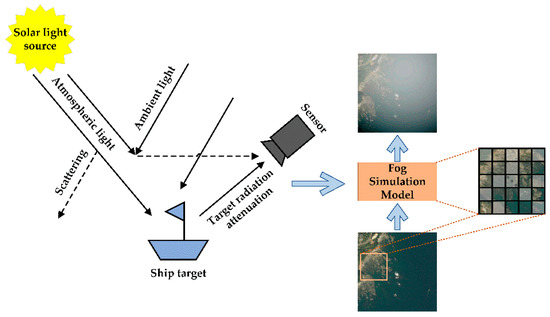
Figure 1.
Fog simulation based on the optical model.
Considering the impact of noise on transmission, fog consistently exhibits spatial randomness and density nonuniformity. Therefore, we established the random diffusion of regional noise brightness. The input image was divided into different regions , and parts of the regions were randomly selected to participate in the diffusion processing. Based on the principle of center point diffusion, the diffusion degree at pixels (j, k) is defined as follows:
where (m, n) is the central point of the region . It can be inferred that the closer to the center point, the higher the diffusion degree value.
Considering the impact of the distance from the camera to the scene on transmission, unlike common scenes, the top-view angle of remote sensing results in minimal spatial distance differences between the foreground and background. Strictly speaking, the difference is preserved and regarded as a weak distance attenuation. In the case of random diffusion noise, transmission transmittance is defined as distance attenuation:
where β represents the attenuation factor, which effectively controls the thickness of the fog: the smaller the attenuation factor, the thicker the fog is. According to the theory of semantic foggy scene understanding [55], the attenuation factor always obeys . In this experiment, for convenience, β was limited in set S: {0.01 0.02 0.04 0.06 0.08 0.12 0.16}.
Global atmospheric light is related to lighting and is often set as a relative value. In this experiment, considering different lighting conditions, global atmospheric light was randomly selected in set T: {0.8 0.85 0.9 0.95 1}. Finally, the fog simulation was added to part of the data to improve the generalization performance of the model.
2.2. The Proposed LMSD-Net
Most lightweight frameworks mainly consider factors such as parameter size and computation complexity. Some models [45,56] achieve less computation complexity but sacrifice accuracy. Therefore, it is important to design a framework focusing on both lightweight and high performance. In this section, we proposed a lightweight multi-scale ship detector network (LMSD-Net) that can simultaneously locate and classify ship targets in ORSI, especially small-target ships.
2.2.1. Overall Architecture
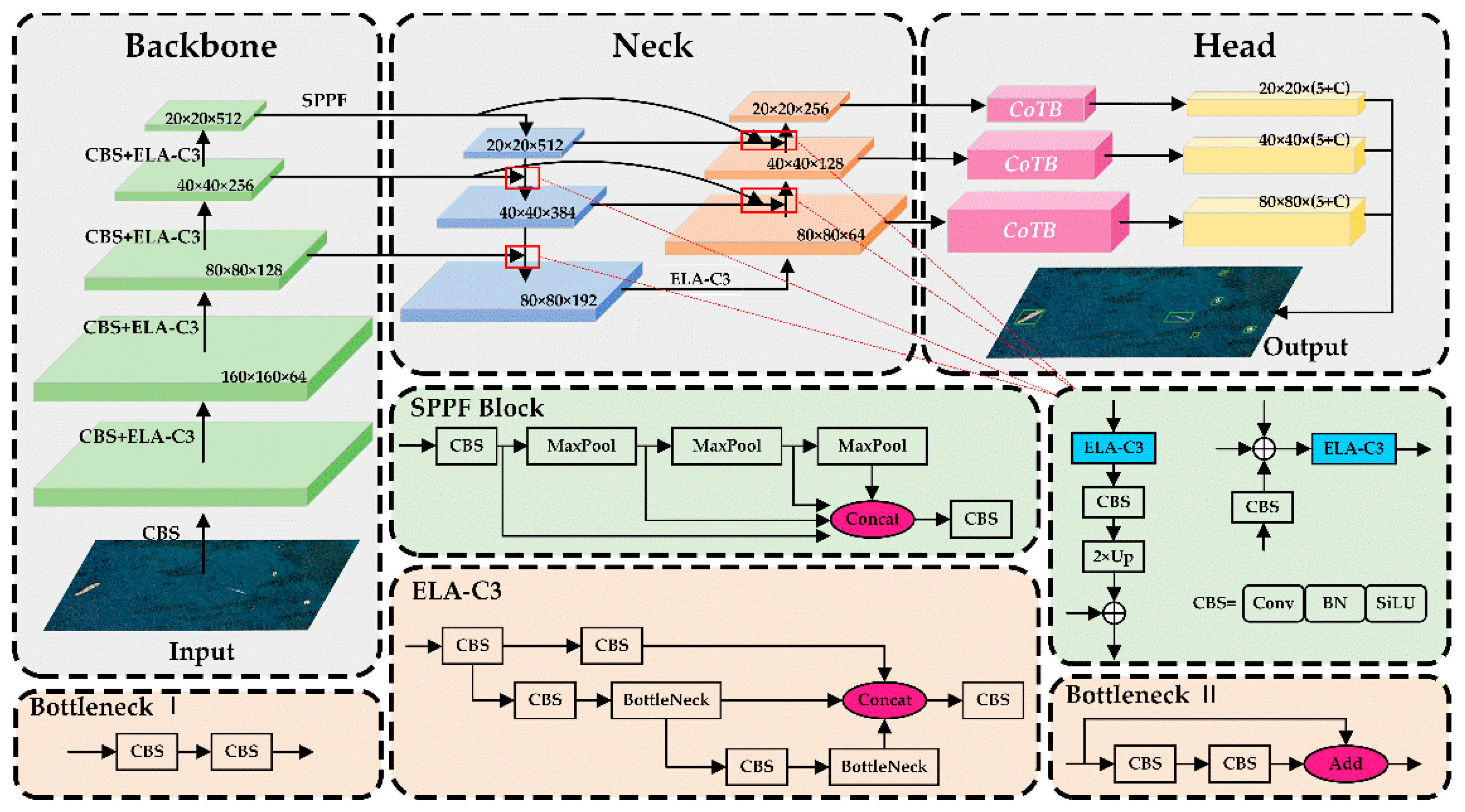
Based on the classic detection paradigm, the overall architecture consists of three parts shown in Figure 2. The first part is a CNN backbone, which extracts feature maps of different layers. The second part is a bidirectional fusion process based on feature pyramids, and the third part includes a detection head used to predict the categories and bounding boxes of ships.

Figure 2.
Overall architecture of the LMSD-Net framework.
In terms of the architecture backbone, we continued the idea of the YOLO series models, which have proven their strong feature extraction capabilities in detection and other issues. It is worth noting that, unlike the C3 module (Yolov5), Repvgg Block (Yolov6), and E-LHAN (Yolov7), we designed a new functional module (ELA-C3 Block). Rethinking C3 and bottleneck-CSP, we added a branch containing Bottleneck structural units. After branch expansion, ELA-C3 Block has a more efficient feature extraction ability than C3.
Regarding the architecture neck, we proposed an improved fusion structure with a weighted-channel network (WFC-PANet). In WFC-PANet, the features of different channels are given weighted specificity. In addition, we abandoned the principle of equal channels for feature aggregation but designed half of the convolutional kernels to control the number of channels. Therefore, the number of channels for fused features was reduced to half of the original number, greatly reducing the parameters and Floating Point Operations (FLOPs).
In the detection head, a Contextual Transformer encoder (CoT) was added to effectively locate targets, further improving the detection performance of small ships. Thus, a more detailed network structure is shown in Table 1.

Table 1.
Information about each layer of the LMSD-Net structure.
Each row in Table 1 represents the forward propagation of the corresponding feature layer. By executing the corresponding number of modules, the shape of the feature output is marked in the “Output Shape” and the parameters are recorded in the “Params”. “Num” represents the number of repetitions. For example, in the sixth row of the table, the features of the fourth layer of the network will be used as the input of the ELA-C3 module to further extract the features, the extracted feature scale is 80 × 80 × 128, and the number of process parameters is 115,712. From the output shape of the 24th–26th rows, the model provides three scales of feature output, which would serve for multi-scale ship detection. From the output shape and “Params” of the 17th, 20th, and 23rd rows, the improved feature fusion part preserves small parameters and channels. The last line summarizes the model’s convolution layers, total parameters, and computational complexity values.
2.2.2. Efficient Layer Aggregation Block
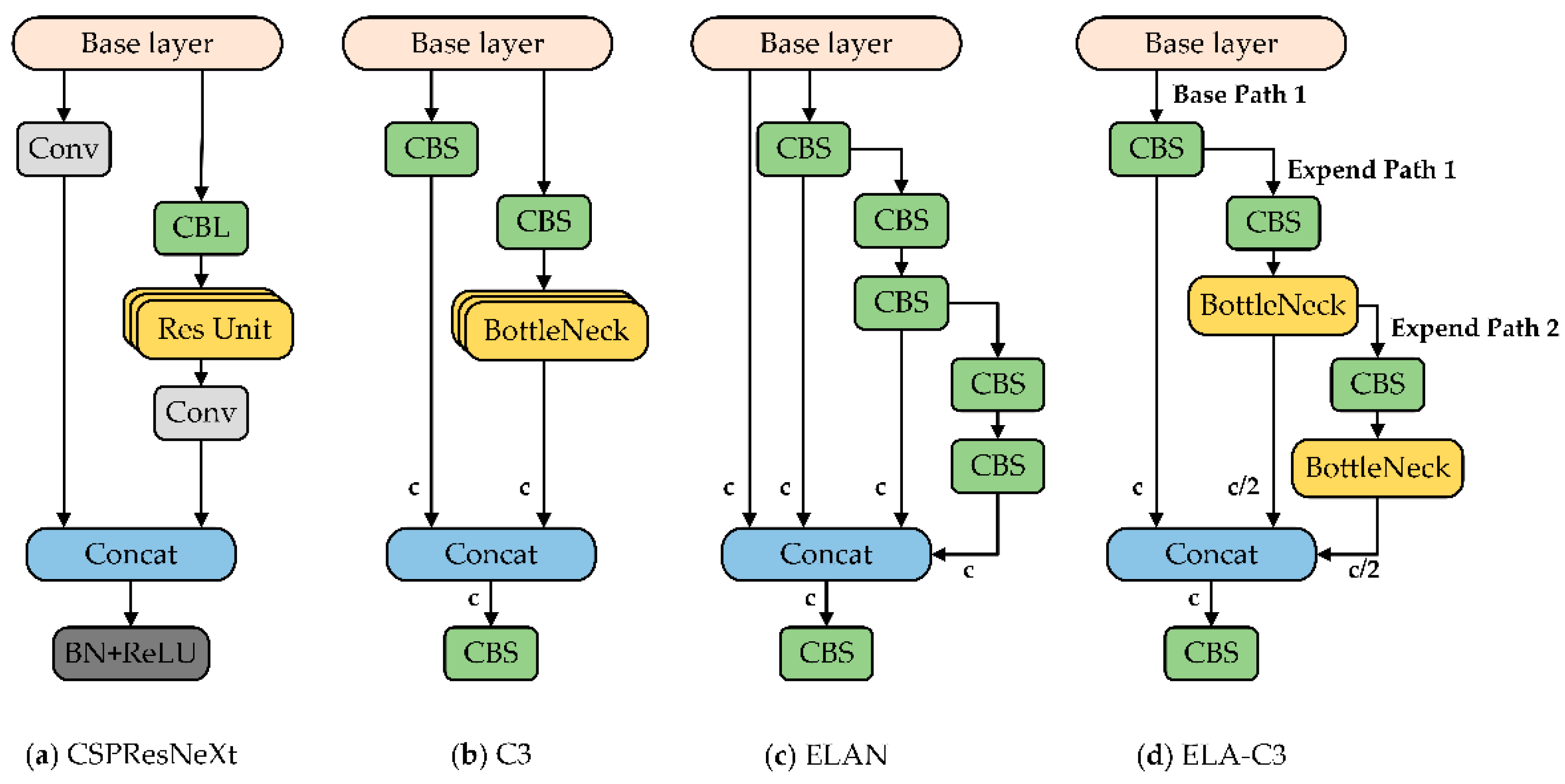
The backbone and neck focus more on obtaining efficient features, especially in lightweight models. As shown in Figure 3a,b, C3, as a variant of CSP-ResNeXt, still retains the CSP architecture and adopts CSP-Bottleneck as the modified unit with fewer parameters. In lightweight models, sharing current layer weights often achieves efficient layer aggregation. Based on this idea, we proposed a variant named Efficient Layer Aggregation of C3 (ELA-C3) in Figure 3d. In addition to reducing repetitive gradient learning, we also analyzed the gradient path. Compared to the Efficient Layer Aggregation Network (ELAN) [29], ELA-C3 removes the base layer paths with less contribution and assigns different channel numbers to different layers. For example, in Figure 3d, the number of channels in the three paths from left to right is c, c/2, and c/2, respectively. In this way, different layers can learn more various features without damaging the original gradient path, which is beneficial in enhancing learning ability.

Figure 3.
Evolution and exploration of the ELA-C3 module.
From the perspective of gradient diversion, the base path only performs ordinary transformations, while the two extended paths use efficient transformations to obtain extended features. Based on group convolution, ELA-C3 forms a local “extend–transform–merge” structure. Assume that feature x is obtained from the base path by the CBS operation. On the one hand, x is exported to participate in the final merger. On the other hand, x serves as the input for extended path features. In Extension Path 1, x performs an efficient transformation to obtain ψ(x). Then, ψ(x), as the input of Extension Path 2, participates in an efficient transformation of c/2 convolution kernels. Finally, the output results are merged by concatenating operations. The “split–transform–merge” structure can be expressed as follows:
where represents the merge operation, and represents the efficient transformation. Output of the structure has c channels.
In the implementation, we adopted group convolution (group = g) to expand the channel and cardinality of the computational block. First, we applied the same parameters and channel multipliers to the two extended paths. Then, we concatenated the tensors of the three paths together. The number of channels in each group of feature maps will be the same as that in the base layer. Finally, we added g sets of feature maps to obtain the complete features. Therefore, ELA-C3 could construct efficient layer aggregation blocks by group convolution to learn more diverse features.
2.2.3. Lightweight Fusion with Weighted-Channel Concatenation
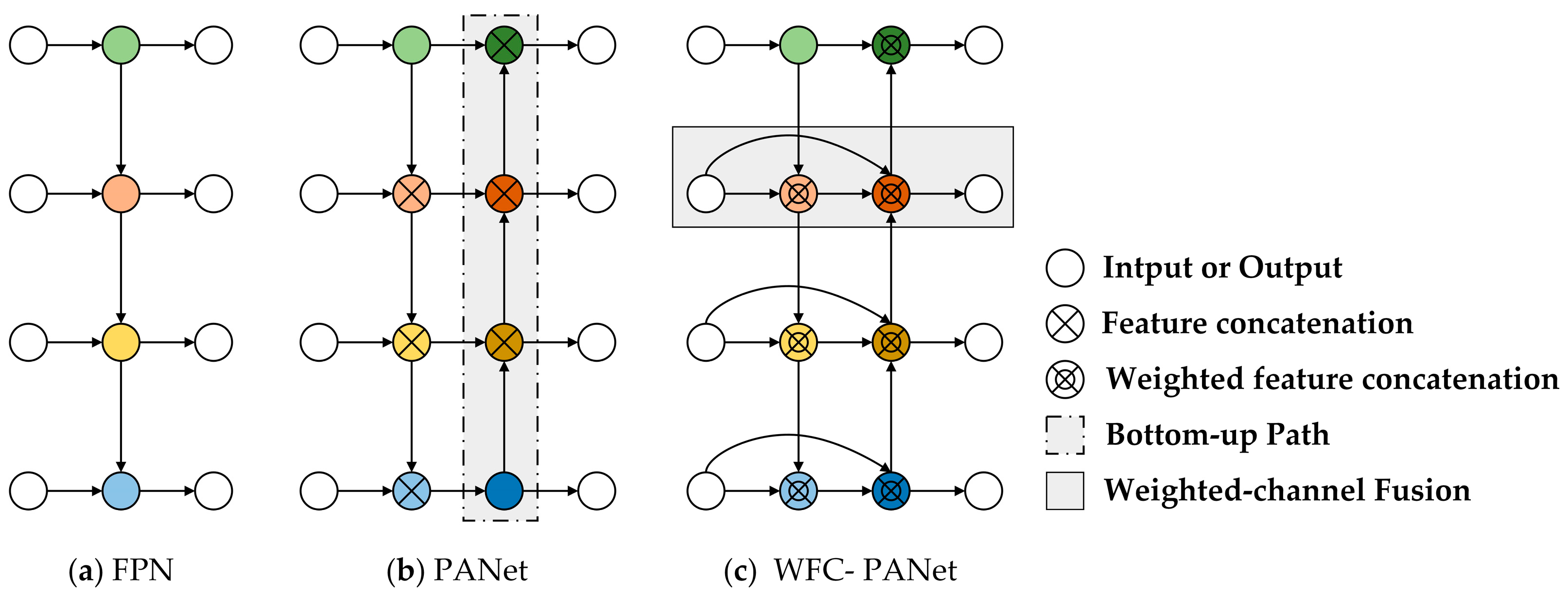
For the single-stage detector, multi-layer detection is an important method to address scale differences. As we all know, FPN has inconsistency of features among the different scales of the target. Specifically, large targets are typically associated with higher-feature maps, while small targets are typically associated with lower-feature maps. After sampling and fusion, the high-level feature responsible for large targets has rich semantic information but fuzzy spatial information. In contrast, the low-level feature responsible for small targets has an accurate location but less semantic information. This may result in a low classification accuracy for small targets and an inaccurate positioning for large targets. In Figure 4b, PANet adds a bottom-up fusion path, which is a “soft fusion” to ensure that spatial features are mapped to global features. However, not only does it bring more parameters and computational complexity, but also the loss from sampling is irreparable. For these issues, we proposed a lightweight fusion with the weighted channel based on PANet (WFC-PANet).
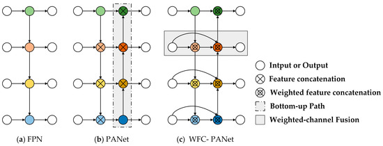
Figure 4.
Fusion structure improvement of WFC-PANet.
Specifically, WFC-PANet adds learnable weights to all the channels in bidirectional fusion. Since different feature maps have different resolutions before stacking or adding, their contributions to the fusion are also different. Therefore, we established a feature competition mechanism based on the contribution to the fused feature map. Once a channel becomes more important in the fusion of features, it will occupy a greater weight. Then the weight is expressed by a fast normalization fusion formula:
where and for stabilizing the value. Then, the number of channels of the output features is reduced to half of the original features, which avoids the reuse of similar features and reduces training parameters. Although it sacrifices some of the compelling features, the cross-layer weighted concatenation basically guarantees the expressiveness of the fusion.
To illustrate the fusion in Figure 4c, we used the concept of set to describe the features. As shown in Figure 5a, the entire detection neck is divided into three layers horizontally and three columns vertically. The available feature sets X, Y, and Z contain three scales of feature maps with different receptive fields. Then, based on the number of branches, the fusion includes two specific forms: two-node fusion and multi-node fusion. In Figure 5b,c, external mapping expands the fusion scales, while internal mapping only increases the diversity of features. Multi-node fusion adds cross-layer weighted fusion compared to two-node fusion. Because of more available feature map choices, multi-node fusion will be more inclined to select efficient features. Therefore, it seems this part of the features is screened and participates in feature refactoring. Moreover, both of them adopt Formula 5, and the values of each normalized weight are limited to [0, 1]. As for the layers corresponding to set Y, two-node weighted fusion is used. For example, the layer is generated by the weighted fusion of corresponding and in the X set. As for the feature layers corresponding to set Z, multi-node weighted fusion is used because of the addition of cross-layer channels. For example, is generated by weighted splicing of , , and .
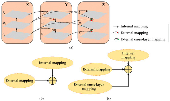
Figure 5.
Abstract representation of fusion mapping. (a) Schematic diagram of a bidirectional fusion set. (b,c) Specific integration forms. The available features include the native feature set X, the top-down feature set Y, and the bottom-up feature set Z.
2.2.4. Contextual Transformer Block for the Detection Head
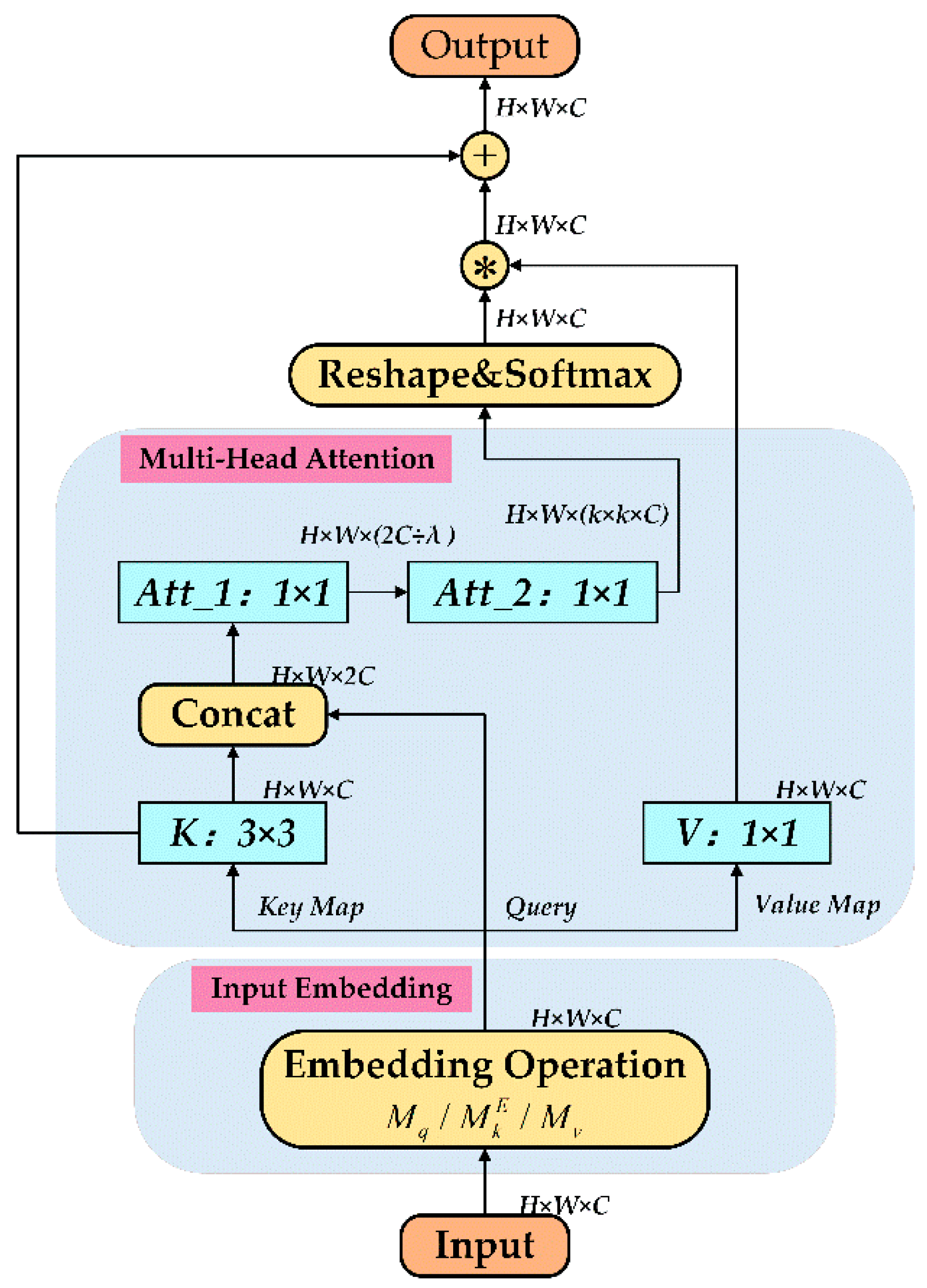
Discrete convolution operators impose spatial locality variance, which is beneficial for reflecting local differences. However, the limited acceptance field affects the modeling of global relationships and makes it less apparent to the remote feature interactions. Inspired by visual transformers, interactions in pairs of queries and keys can measure the global attention matrix, which reflects contextual self-attention expression well. Based on CNN, we added a lightweight Contextual Transformer (CoT) block before the shared decoupled head for more accurate classification and localization.
Specifically, as shown in Figure 6, given a ship feature map , it can be transformed into queries, keys, and values, which are defined as follows:
where , , and are the embedding matrices, which transform the sparse image into a dense matrix. Assuming the central key of the context area is , the surrounding key is the region with k × k (k = 3 in Figure 6). Centered around each key in the surrounding area, the k × k convolution can calculate the contextual information of each key. Similar to sliding window convolution in CNN, the learned contextual key reflects the static information of the center and surrounding.

Figure 6.
Measurement of the attention matrix in the CoT block.
Then, the learned contextual keys and queries are concatenated to synthesize new keys []. By using two consecutive 1 × 1 convolutions to perform self-attention:
where represents the convolution with SiLU while represents the convolution without activation. Obviously, the learned attention weight matrix considers the context keys and queries. In other words, the purpose of mining contextual information is to improve the self-attention of local regions. Next, Softmax is used to form the attention weight matrix . Aggregating the value matrix, a dynamic contextual self-attention weight matrix is calculated and represented as follows:
During the forward transmission process, static context and dynamic context integrate through the overlay fusion mechanism [57]. The hardware algorithm implementation is shown in Figure 7.
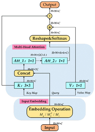
Figure 7.
The detailed structures of the Contextual Transformer (CoT) block. denotes local matrix multiplication, and denotes the fusion of dynamic and static keys. For two consecutive 1 × 1 convolutions, channel scaling factor λ is set as 4 in the experiment.
Essentially, CoT is a self-attention block that combines transformers. Therefore, treating CoT as a convolution module is feasible. In the ablation experiment, we increased the number of CoT blocks to obtain the best response.
2.2.5. Prediction
As mentioned above, three prediction branches are elicited to accurately detect multi-scale ships. In the output of each branch, the positive sample grids, which are used to predict the real target, need to be filtered and serve for location prediction. Since the ship targets are mostly distinctly elongated, the aspect ratio of the label has a positive effect on the prediction. In addition, we expanded the prediction location to three cell grids to filter positive samples with a multi-sample label matching strategy [27]. In this way, the labels are assigned to all the anchors simultaneously during training, thus alleviating the problem of unbalanced positive and negative samples during training to some extent. Once the positive samples are identified, the positive sample loss is calculated as the sum of grid confidence loss, target classification loss, and target bounding box regression loss. The negative samples only need to calculate the confidence loss.
In the training process, we inherited the Binary Cross-Entropy as the class loss and confidence loss of the positive and negative samples of the grid. Considering the prediction output grid (S × S), each cell in the grid generates N bounding boxes, whose center coordinate is (x, y), prediction confidence is c, and the prediction vector points to the kth class with prediction value . Class loss and confidence loss are defined as follows:
where , are the truth of p, c. denotes whether the object appears in the bounding box j predictor in cell i. It is worth noting that the positive sample only contains three grids, while the negative sample contains other grids as well as grids from other detection layers. Due to the labels of the negative samples , the confidence loss calculation for negative samples can be optimized approximately as follows:
For the bounding box regression loss of positive samples, we proposed an improved version named V-CIoU based on CIoU [58]. First, consider the formula of CIoU:
where B and represent the areas of the prediction box and the ground-truth box, respectively, (, , , ) is the matched truth value of (x, y, w, h), c is the diagonal length of the smallest closed box covering both boxes, α is the weight parameter, and v is the penalty representing the aspect ratio’s consistency.
CIoU loss adds the distance offset and aspect ratio of the prediction box to the IoU, and both of them are beneficial for improving the regression accuracy of the ship. However, a problem that needs to be considered is that the penalty term v in Formula (16) will fail when the aspect ratio of the truth and prediction is equal or approximately equal. Especially for some small-ship targets, the similar aspect ratio results in incomplete convergence. In this case, we proposed a penalty function based on the variance of the ground truth and the prediction for each corresponding aspect ratio. This penalty term u is defined as follows:
The penalty term v is preserved as a part of the new penalty function. Normally, the penalty term v can solve the problem of offset. The variance penalty term is activated when the ratio between the prediction and the ground truth is consistent. Therefore, V-CIoU not only embodies the advantages of CIoU but also solves the degradation problem, in that the aspect ratio of the ground truth equals that of the prediction. Once the aspect ratio of the prediction and ground truth are maintained within a small range, the convergence behavior reaches its limit, and then the penalty loses efficacy. Finally, the bounding box regression loss is defined as follows:
Furthermore, the implementation process is summarized in Algorithm 1.
| Algorithm 1. V-CIoU computation | |
| 1: | Input: Bounding box of ground truth |
| 2: | Input: Bounding box of prediction |
| 3: | Output: VCIoU between the ground-truth box and the prediction boxes |
| 4: | If do |
| 5: | For A and B, find the smallest enclosing convex object C. |
| 6: | within C, calculate . |
| 7: | If : |
| 8: | then , |
| 9: | , |
| 10: | . |
| 11: | else |
| 12: | then . |
| 13: | else |
| 14: | . |
3. Results and Experiments
This section provides a detailed introduction to the dataset and a description of the evaluation metric. Then, we conduct a large number of experiments to demonstrate the effectiveness of the framework. On the one hand, we perform ablation experiments for the proposed data argument and self-designed modules with relevant advanced methods. On the other hand, we perform a detailed comparison with the current excellent lightweight detection frameworks. Finally, the detection results using the most advanced methods are presented, leading to a profound discussion in the next section.
3.1. Dataset
The increase in high-resolution optical images has greatly contributed to the advancement of target detection. Improving the detection performance of small ships relies on collecting small-target ship datasets. However, existing open data sources still need to be extended in the diversity of scenes and targets. For example, in HRSC2016 [59], there are only two or three targets in an image, most of which are large-scale targets. The scenes of NWPU VHR-10 [60] and the Airbus ship dataset [61] are more singular with the coastal background. Subsequently, we have proposed the VRS ship dataset [54] (VRS-SD) in our previous study, which contains various maritime disturbances, such as thin clouds, islands, sea waves, and wake waves. Therefore, the application of VRS-SD is oriented toward detection tasks in maritime scenes. In order to meet the unified detection requirements for nearshore and maritime scenes, we furthermore construct VRS-SD v2, which covers different nearshore scenes, marine environments, maritime disturbances, target scales, and dense small-target distributions. The detailed differences among the current datasets are summarized in Table 2.

Table 2.
Comparison of ship datasets.
According to the statistics in Table 2, most of the existing ship datasets are from Google Earth and are mostly taken under sunny conditions. Both VRS-SD and VRS-SD v2 are collected under a variety of weather conditions. Compared with VRS-SD, VRS-SD v2 has significantly expanded the amounts of images, and the two additional classes are near-shore ships and river-distribution ships. In addition, to address the problem of insufficient fog interference background in VRS-SD, we provided more images of such scenes through fog simulation. Since AI-TOD focuses more on the differences in nearshore target scale, it usually better reflects the complexity of the scenes. Therefore, in the final validation, we implemented our method on the AI-TOD dataset.
3.1.1. The Analysis of VRS-SD v2
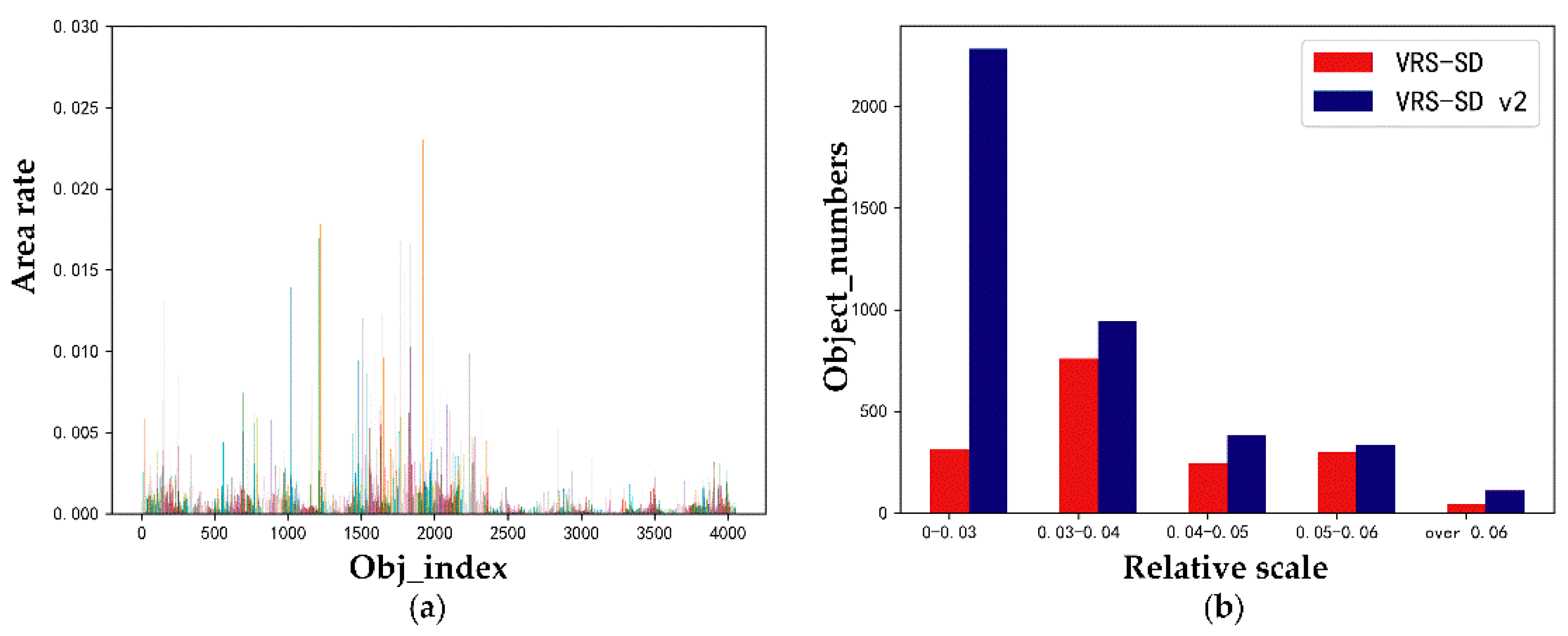
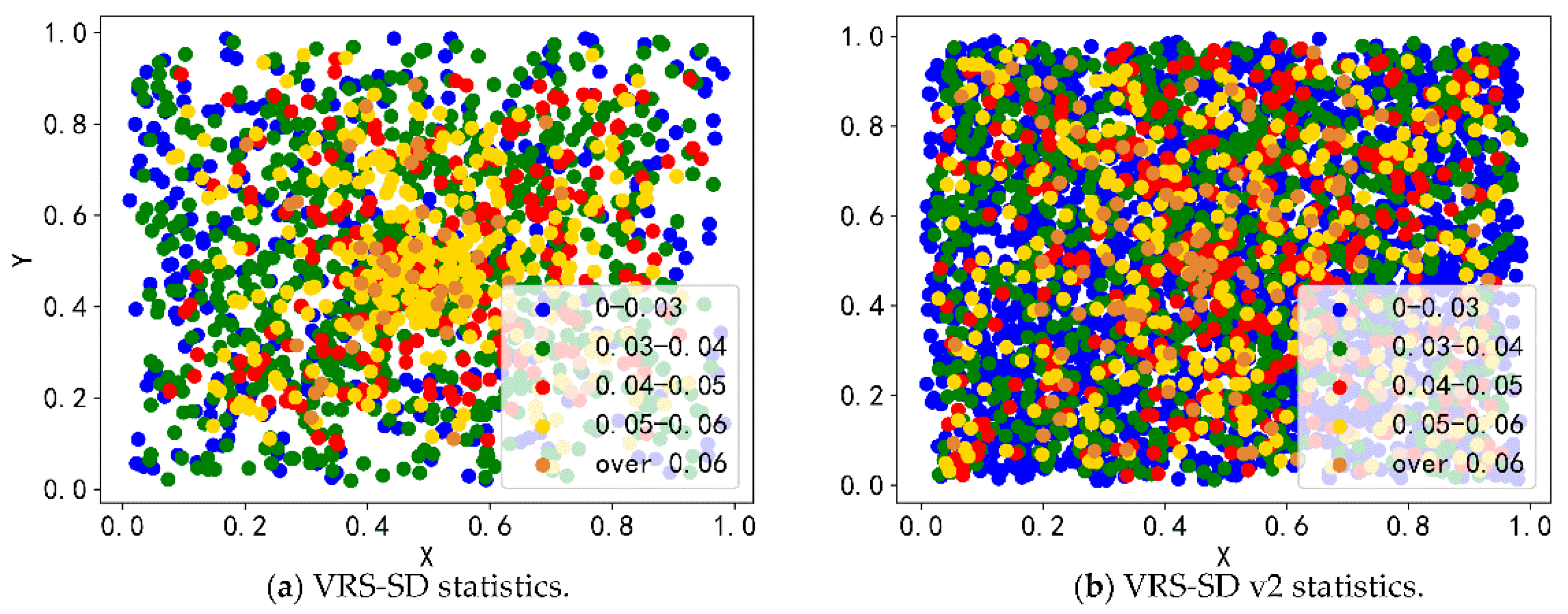
VRS-SD v2 increases the number of ship targets at different scales. To compare the targets at different scales, we first refer to the definition of the small target. The small-target scale has different absolute definitions in different remote sensing datasets. For example, the MS COCO dataset defines small targets within 32 × 32 pixels. TinyPerson [65] defines small targets as those with pixel values in the interval [20, 50]. Furthermore, the aerial image dataset DOTA [66] defines a small target with pixel values in the range of 10–50. It is difficult to unify the definition of small targets for different datasets, so we introduced a relative definition of small-target scale. Ref. [67] states that the relative areas of small-target instances in the same class, the median ratio of the area of the ground truth to the image, should be limited to between 0.08% and 0.58%. In addition, the ratio of the target bounding box area to the image area is open-squared to less than a certain value, the more general value being 0.03. Based on the above considerations, we compared the two datasets at a finer scale as shown in Table 3. It can be seen that there is a significant increase in tiny ships, and the number of small targets has increased to varying degrees at the subdivision scales. Figure 8 counts the relative areas of all ship instances and the number of targets in different intervals. In addition, Figure 9 shows the distribution of ship positions at different scales, and VRS-SD v2 has more targets and a denser distribution.

Table 3.
Quantitative statistics of multi-scale ships.

Figure 8.
Target statistics of VRS-SD v2 and comparison with VRS-SD. (a) Relative scale statistics in VRS-SD v2. (b) Comparison of target-relative scale distribution between VRS-SD and VRS-SD v2.
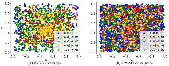
Figure 9.
Distribution of target positions at different scales in VRS-SD and VRS-SD v2. The X and Y axes indicate the relative positions of the ships, and the image scale is normalized to a relative scale of 1.0 × 1.0. Different colors indicate the targets at different scales.
3.1.2. Fog Simulation
VRS-SD v2 includes a few cloud images and fog images. We performed the fog simulation on a certain proportion of images to simulate the real-world detection background. These images have been fogged at random spatial locations with varying degrees. In Figure 10, we present some simulation examples of some typical scenes. The fog simulation in the coastal area represents the real situation. Once the model is trained to resist the disturbances caused by fog, it can be deployed to industrial equipment, especially those devices under severe weather conditions.
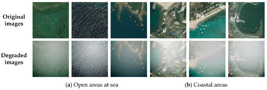
Figure 10.
Examples of fog simulation. (a) The open areas contain lakes, island shores, and sea clutter. (b) The coast scene with dense ship targets.
3.2. Evaluation Metrics
Similar to the general target detection task, we used precision rate, recall rate, and average precision to evaluate the performance of the proposed network. By setting a threshold for the intersection over union (IoU), the prediction results can be filtered and divided as true positive (TP), true negative (TN), false positive (FP), and false negative (FN). The formulas for precision, recall, and F1 score are as follows:
Furthermore, average precision (AP) calculates the total precision of the recall value from 0 to 1, that is, AP is the area enclosed by the P-R curve and the coordinate axis. Let r be the recall rate and P(r) be the accuracy corresponding to the curve. By interpolation, AP as the line integral is calculated as follows:
For the lightweight comparison, we use the GFLOPs and parameters, which could reflect the network complexity and memory usage. Additionally, frames per second (FPS) is calculated to quantify the detection speed. In consideration of the limitation of the device, FPS is tested with batch size = 1 or 16 in the experiments.
3.3. Ablation Study
All the experiments were tested and evaluated on a computer with an Intel Core i7-10900 2.90 GHz CPU, 24 GB memory, and GeForce GTX 3060Ti GPU with 8 GB. In the preparation phase, the dataset was divided into a training set, a validation set, and a test set in a ratio of 8:1:1. By k-means clustering, the criteria for the three classes of anchors were automatically generated based on the ship scale in the specific dataset. During the training process, we applied the AdamW optimizer and trained 200 epochs to ensure convergence. For all experiments, the IoU was set to 0.6.
3.3.1. Effect of Fog Simulation
To verify the importance of fog simulation for practical detection work, as shown in Table 4, we tested the fog simulation on MASATI and VRS-SD v2, which are both the small-ship dataset. It is worth noting that we set three rates, 0, 50%, and 100%, to test the effect of fog simulation on the results. The best results of the three rates are highlighted in red.

Table 4.
Fog simulation for data enhancement.
Taking MASATI as an example, the model can give the best results at AP@0.5 of 0.813 and AP@0.5:0.95 of 0.407 without fog interference. However, when the training set lacks fog images, the testing achieves the worst results, with AP@0.5 of 0.587 and AP@0.5:0.95 of 0.264. Adding a certain percentage of fog images in the dataset can match the real remote sensing detection and improve the robustness of the model to weather conditions. On VRS-SD v2, when the training and test sets are mixed with fog images simultaneously, the detection results are better than the in case of all fog images, and AP@0.5 and AP@0.5:0.95 reach 0.741 and 0.342. It also provides an experimental basis for obtaining the best ratio of fog images.
3.3.2. Effect of ELA-C3
ELA-C3 is an improved version of the C3 module. To verify the validity of ELA-C3, we used C3 as a baseline in LMSD-Net. Additionally, we applied all remaining components of LMSD-Net. As shown in Table 5, the model obtains results by replacing the C3 module in the backbone and neck.

Table 5.
Ablation of ELA-C3.
When ELA-C3 is added to the backbone or neck, the AP@50 values are 3.9% or 1.5% higher than the baseline model. In addition, the AP value with ELA-C3 exclusively is 5.5% higher than that using C3. As a lightweight feature extraction module, ELA-C3 has less increase of parameters. Therefore, the ELA-C3 module facilitates the efficient acquisition of rich contextual spatial features to improve the detection performance of ship targets.
3.3.3. Effect of WFC-PANet
In the detection neck, we designed the cross-layer and weighted-channel concatenation based on PANet. To avoid the influence of ELA-C3, all the following networks uniformly used the Yolov5s-backbone. Then, we quantified the experimental results of the current advanced feature fusion methods in Table 6.

Table 6.
Comparison of different feature fusion methods in the neck.
The experiment results show that using WGC-PANet leads to an increase in speed and a more lightweight model. In addition, there is a small sacrifice in average accuracy compared with PANet. Nevertheless, the model still maintains good performance and enough to finish the detection task. Similar to BiFPN, WGC-PANet also mentions a cross-layer connection. However, the use of adding BiFPN increases the computation complexity significantly. On the contrary, using Concat guarantees the model’s performance and reduces the computation complexity. Taken together, the cross-channel and weighted-channel concatenation adopted by WGC-PANet can maintain the model’s expressiveness and provide the possibility of lightweight implementation.
3.3.4. Structure Exploration of the Detection Head
The prediction head is crucial for the decoupling of the feature map. Based on the general structure of LMSD-Net, the comparison results of applying different mainstream detection heads are presented in Table 7. Further, to explore the effect of the number of CoT blocks, we embedded different numbers of CoT blocks and obtained the optimal choice according to the comparison. Note that CoT_x denotes the use of x CoT blocks.

Table 7.
Exploration and comparison of detection heads.
In the YOLO head, the classification and localization branches are fused to share the convolutional layers. In the decoupled head, the two branches are convolved separately to obtain higher accuracy. Therefore, applying the YOLO head has fewer parameters and computation complexity than the decoupled head but poorer performance. With the addition of CoT blocks, the detection performs more powerfully. Compared with Swin Transformer block, CoT_3 obtains less computation complexity as well as higher precision. In addition, the number of CoT blocks affect the performance. More CoT blocks will bring a slight increase in parameters and GFLOPs but a decrease in speed. Considering the performance and hardware consumption, we finally chose CoT_3 in the network.
3.3.5. Validation of Regression Loss Function
According to the analysis of VRS-SD v2 in Table 3, the relative area ratios of tiny and small targets are primarily of [0,0.0016]. Therefore, the observation will have a similar aspect ratio between the ground truth and the predicted bounding box, which leads to the failure of the aspect ratio penalty term of CIoU. To verify the validity of the proposed variance penalty term for V-CIoU, we designed experiments of regression loss, as shown in Table 8. We set three different thresholds for the following loss functions in the valid. On the whole, V-CIoU has the best effect. Compared with CIoU, V-CIoU improves by 2.9% at AP@75 and 2.2% at AP@50:95. The experiments demonstrated that adding the variance penalty term makes V-CIoU more adaptable to tiny- and small-ship detection.

Table 8.
Validation of the improved V-CIoU.
3.3.6. Multi-Scale Performance of the Model
Based on the statistics of the dataset, the proposed VRS-SD v2.0 contains ship targets that are mostly small- and medium-sized, whereas VRS-SD proposed in previous work contains more large targets. Therefore, we combined the two datasets to explore the model’s detection performance for different-sized ship targets. Table 9 lists the comparison results of the lightweight SOTA detectors.

Table 9.
Comparison of detection performance at different scales.
From the results, we see that LMSD-Net is comparable to the latest Yolov6-3.0n in terms of being lightweight, while LMSD-Net performs better on small targets and medium-sized targets, with an improvement of 5.6% and 7.8%, respectively. Considering this enhancement, on the one hand, the small and medium targets are well trained due to the large number of small and medium samples in the dataset. On the other hand, V-CIOU specifically solves the problem of the inconsistent aspect ratio of small targets, thus improving detection accuracy. In addition, the AP for large-ship targets reaches 0.644, which is lower than Yolov8s by about 3.9%. Nevertheless, the parameters of LMSD-Net are only half of those of Yolov8s, and the computation is reduced by 45%.
3.4. Overall Detection Performance
To validate the overall detection performance, we first compared the proposed models with the current lightweight state-of-the-art on the VRS-SD v2. These comparison methods include lightweight versions of the universal detectors, such as EfficientDet (D0-D3), Yolov7-tiny, and Yolov8n, and specialized lightweight detectors, such as the Nanodet family. In addition, we added a variant of Yolov5s called Yolov5-Ghost, which introduces the lightweight backbone GhostNet into the CSP architecture. For this part of the experiments, we used the training and validation setup of the ablation study. To ensure great and fast convergence, we increased the pre-training weights and performed 200 epochs of training. In addition, we set the batch size = 1 to test the general real-time performance. The comparison experiments were fair and extensive. We directly trained and tested all the comparison methods using official open-source codes.
Generally, as shown in Table 10, the proposed method performs best on this small-ship dataset. In terms of AP@50, LMSD-Net achieves the highest value with 81.3%. Compared with Yolov8s and Yolov6-3.0-s, which have high average accuracy, LMSD-Net has more advantages in terms of parameters and computation complexity. Therefore, it can meet the needs of ship-target detection tasks better. In addition, we observed that parts of the anchor-free detectors in Table 10, like Yolov6s-3.0 and Yolov8s, performed better than the Yolov5 series, Yolov4-tiny and Yolov7-tiny, which are anchor-based detectors. Since tiny targets are more sensitive to IoU than large targets, the anchor-based detectors, such as Yolov7-tiny and Yolov5n, cannot accurately predict the bounding box. Especially in AP@50:95, which has a stricter limitation than AP@50, common IoU loss will lead to less improvement. With the proposed V-CIOU, we could improve the average accuracy and cope with the tiny-target detection.

Table 10.
Comparison of the lightweight SOTA performance on VRS-SD v2 (30% foggy images).
In terms of lightweight, the Nanodet series perform the best. However, they are mainly applied to mobile target detection and are not well adapted to small-ship target detection in the remote sensing field. Due to the small model input scale, such as or , the feature description capability is limited, which leads to low detection accuracy. Differently, the model input scale of the EfficientDet series increases with the expansion of the backbone. Based on DWConv, the scaled model gradually adapts to lightweight but sacrifices more accuracy and improves a little in speed. In contrast, the accuracy advantage of LMSD-Net is very obvious and ensures efficient detection performance.
Although the speed of LMSD-Net is not the fastest, it is acceptable compared to most of the advanced detectors mentioned earlier. Its detection speed reaches 68 FPS, which could meet the real-time requirement (FPS > 30).
Further, in Figure 11, we show the detection results using LMSD-Net on AI-TOD, MASATI, and VRS-SD v2. It can be observed that our model performs well on all three datasets with no missed and false detections essentially, which indicates that the model has a high generalization ability. Despite the large interference caused by clouds and fog to the ship target, the detection still performs well.
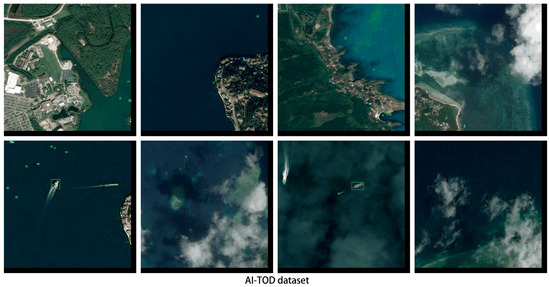
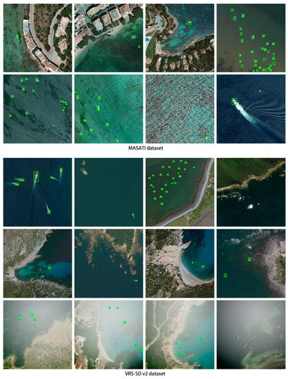
Figure 11.
Detection results of the proposed LMSD-Net on different datasets.
4. Discussion
In this study, we propose a new ship dataset VRS-SD v2, which adds more small- and tiny-ship targets located nearshore and in rivers. The dataset covers different open coast scenes, marine environments, maritime disturbances, target scales, and more dense distributions. In addition, we propose a new fog simulation method for increasing the proportion of fog images in the dataset. This method can improve the robustness of the model in severe weather conditions. We have demonstrated the importance of fog simulation for actual detection by implementing different proportions of fog simulation on the dataset in the ablation experiment.
Then, we propose a new lightweight model (LMSD-Net) specifically for ship detection. In the network, we design the ELA-C3 module for efficient feature extraction. In the feature-fusion process, we propose a fusion method with compressed channels and weighted connections to ensure lightweight and low computational complexity. In the detection head, we introduce a contextual transformer (CoT) block to improve the detection accuracy. In the prediction process, the variance penalty term is added, and the prediction performance is improved for the relative scale consistency of the targets.
Furthermore, we validate the effectiveness of each module and the overall detection performance on two small-ship datasets (VRS-SD v2 and MASATI). The ablation experiments indicate that the ELA-C3 module, CoT block, and V-CIoU are beneficial in improving accuracy. Meanwhile, WGC-PANet mainly enhances lightweight performance while ensuring the expressiveness of the model. The overall comparison demonstrates that the proposed model can reach 81.3% at AP@50 and 38.4% at AP@50:95 in VRS-SD v2, while with only 5.5M parameters and 12.8 GFLOPs. Among the existing lightweight detection models, LMSD-Net has better detection capability for small and tiny ships and achieves SOTA performance. In addition, the detection speed reaches 68 FPS, which could meet the real-time requirement.
5. Conclusions
The proposed lightweight model presents a feasible solution for remote sensing ship detection and project deployment. The model performs well in dealing with complex background disturbances near shore and at sea. Fog simulation has positive implications for ship detection in bad weather conditions. In the future, reducing the computation complexity will remain a challenging research task. In addition, we will further improve our research in weighted-feature fusion and more comprehensive weather simulations. Inspired by the Transformer, we believe that remote feature interaction will be the key to improving detection performance in lightweight ship detection.
Author Contributions
Conceptualization, Y.T. and S.Z.; methodology, Y.T.; validation, Y.T. and S.Z.; investigation, Y.T., F.X. and X.W.; resources, Y.T. and J.L. writing—original draft preparation, Y.T.; writing—review and editing, F.X. All authors have read and agreed to the published version of the manuscript.
Funding
This work was supported by the National Natural Science Foundation of China under Grant 61905240.
Institutional Review Board Statement
Not applicable.
Informed Consent Statement
Not applicable.
Data Availability Statement
Not applicable.
Acknowledgments
The authors are grateful for anonymous reviewers’ critical comments and constructive suggestions.
Conflicts of Interest
The authors declare no conflict of interest.
References
- Zou, H.; He, S.; Wang, Y.; Li, R.; Cheng, F.; Cao, X. Ship detection based on medium-low resolution remote sensing data and super-resolved feature representation. Remote Sens. Lett. 2022, 13, 323–333. [Google Scholar] [CrossRef]
- Cui, D.; Guo, L.; Zhang, Y. Research on the development of ship target detection based on deep learning technology. In Proceedings of the ACM International Conference on Frontier Computing (FC), Turin, Italy, 17–19 May 2022. [Google Scholar]
- Wu, J.; Li, J.; Li, R.; Xi, X. A fast maritime target identification algorithm for offshore ship detection. Appl. Sci. 2022, 12, 4938. [Google Scholar] [CrossRef]
- Yue, T.; Yang, Y.; Niu, J. A Light-weight Ship Detection and Recognition Method Based on YOLOv4. In Proceedings of the 2021 International Conference on Advanced Electronic Materials, Computers and Software Engineering (AEMCSE), Changsha, China, 26–28 March 2021. [Google Scholar]
- Joseph, S.I.T.; Karunakaran, V.; Sujatha, T.; Rai, S.B.E.; Velliangiri, S. Investigation of deep learning methodologies in satellite image based ship detection. In Proceedings of the International Conference on Sustainable Computing and Data Communication Systems (ICSCDS), Erode, India, 7–9 April 2022. [Google Scholar]
- Ding, J.; Xue, N.; Long, Y.; Xia, G.; Lu, Q. Learning RoI transformer for detecting oriented objects in aerial images. In Proceedings of the IEEE/CVF Conference on Computer Vision and Pattern Recognition (CVPR), Long Beach, CA, USA, 15–20 June 2019. [Google Scholar]
- Dalal, N.; Triggs, B. Histograms of Oriented Gradients for Human Detection. In Proceedings of the IEEE Conference on Computer Vision and Pattern Recognition (CVPR), San Diego, CA, USA, 20–25 June 2005. [Google Scholar]
- Felzenszwalb, P.; McAllester, D.; Ramanan, D. A discriminatively trained, multiscale, deformable part model. In Proceedings of the IEEE Conference on Computer Vision and Pattern Recognition (CVPR), Anchorage, AK, USA, 23–28 June 2008. [Google Scholar]
- Wu, X.; Hong, D.; Tian, J.; Chanussot, J.; Li, W.; Tao, R. ORSIm Detector: A Novel Object Detection Framework in Optical Remote Sensing Imagery Using Spatial-Frequency Channel Features. IEEE Trans. Geosci. Remote Sens. 2019, 57, 5146–5158. [Google Scholar] [CrossRef]
- Shi, Z.; Yu, X.; Jiang, Z.; Li, B. Ship Detection in High-Resolution Optical Imagery Based on Anomaly Detector and Local Shape Feature. IEEE Trans. Geosci. Remote Sens. 2014, 52, 4511–4523. [Google Scholar]
- Tang, J.; Deng, C.; Huang, G.; Zhao, B. Compressed-Domain Ship Detection on Spaceborne Optical Image Using Deep Neural Network and Extreme Learning Machine. IEEE Trans. Geosci. Remote Sens. 2015, 53, 1174–1185. [Google Scholar] [CrossRef]
- Zou, Z.; Shi, Z. Ship Detection in Spaceborne Optical Image with SVD Networks. IEEE Trans. Geosci. Remote Sens. 2016, 54, 5832–5845. [Google Scholar] [CrossRef]
- Nie, T.; Han, X.; He, B.; Li, X.; Liu, H.; Bi, G. Ship Detection in Panchromatic Optical Remote Sensing Images Based on Visual Saliency and Multi-Dimensional Feature Description. Remote Sens. 2020, 12, 152. [Google Scholar] [CrossRef]
- Everingham, M.; Van Gool, L.; Williams, C.K.I.; Winn, J.; Zisserman, A. The Pascal Visual Object Classes (VOC) Challenge. Int. J. Comput. Vis. 2010, 88, 303–338. [Google Scholar] [CrossRef]
- Everingham, M.; Eslami, S.M.A.; Van Gool, L.; Williams, C.K.I.; Winn, J.; Zisserman, A. The PASCAL Visual Object Classes Challenge: A Retrospective. Int. J. Comput. Vis. 2015, 111, 98–136. [Google Scholar] [CrossRef]
- Russakovsky, O.; Deng, J.; Su, H.; Krause, J.; Satheesh, S.; Ma, S.; Huang, Z.; Karpathy, A.; Khosla, A.; Bernstein, M.; et al. ImageNet large scale visual recognition challenge. Int. J. Comput. Vis. 2015, 115, 211–252. [Google Scholar] [CrossRef]
- Deng, J.; Dong, W.; Socher, R.; Li, L.; Li, K.; Li, F. ImageNet: A large-scale hierarchical image database. In Proceedings of the IEEE Conference on Computer Vision and Pattern Recognition (CVPR), Miami Beach, FL, USA, 20–25 June 2009. [Google Scholar]
- Lin, T.Y.; Maire, M.; Belongie, S.; Hays, J.; Perona, P.; Ramanan, D.; Dollar, P.; Zitnick, C.L. Microsoft COCO: Common Objects in Context. In Proceedings of the European Conference on Computer Vision (ECCV), Zurich, Switzerland, 6–12 September 2014. [Google Scholar]
- He, K.; Zhang, X.; Ren, S.; Sun, J. Spatial pyramid pooling in deep convolutional networks for visual recognition. IEEE Trans. Pattern Anal. Mach. Intell. 2015, 37, 1904–1916. [Google Scholar] [CrossRef] [PubMed]
- Dai, J.; Li, Y.; He, K.; Sun, J. R-FCN: Object Detection via Region-based Fully Convolutional Networks. In Proceedings of the Conference on Neural Information Processing Systems (NIPS), Barcelona, Spain, 5–10 December 2016. [Google Scholar]
- Ren, S.; He, K.; Girshick, R.; Sun, J. Faster R-CNN: Towards Real-Time Object Detection with Region Proposal Networks. IEEE Trans. Pattern Anal. Mach. Intell. 2017, 39, 1137–1149. [Google Scholar] [CrossRef] [PubMed]
- Hu, J.; Zhi, X.; Jiang, S.; Tang, H. Supervised Multi-Scale Attention-Guided Ship Detection in Optical Remote Sensing Images. IEEE Trans Geosci Remote Sens. 2022, 60, 1–14. [Google Scholar] [CrossRef]
- Lin, T.-Y.; Goyal, P.; Girshick, R.; He, K.; Dollar, P. Focal Loss for Dense Object Detection. IEEE Trans. Pattern Anal. Mach. Intell. 2020, 42, 318–327. [Google Scholar] [CrossRef]
- Zhou, X.; Wang, D.; Krhenbühl, P. Objects as Points. arXiv 2019, arXiv:1904.07850. [Google Scholar]
- Redmon, J.; Farhadi, A. YOLOv3: An Incremental Improvement. arXiv 2020, arXiv:1804.02767. [Google Scholar]
- Bochkovskiy, A.; Wang, C.; Liao, H. YOLOv4: Optimal Speed and Accuracy of Object Detection. arXiv 2020, arXiv:2004.10934v1. [Google Scholar]
- GitHub: Ultralytics. YOLOv5-v 6.1. 2022. Available online: https://github.com/ultralytics/yolov5 (accessed on 23 December 2022).
- Li, C.; Li, L.; Jiang, H.; Weng, K.; Geng, Y.; Li, L.; Ke, Z.; Li, Q.; Cheng, M. YOLOv6: A Single-Stage Object Detection Framework for Industrial Applications. arXiv 2022, arXiv:2209.02976. [Google Scholar]
- Wang, C.-Y.; Bochkovskiy, A.; Liao, H.-Y.M. YOLOv7: Trainable bag-of-freebies sets new state-of-the-art for real-time object detectors. arXiv 2022, arXiv:2207.02696. [Google Scholar]
- GitHub: Airockchip. YOLOv8. 2023. Available online: https://github.com/airockchip/ultralytics_yolov8. (accessed on 10 February 2023).
- Wang, B.; Han, B.; Yang, L. Accurate Real-time Ship Target detection Using Yolov4. In Proceedings of the International Conference on Transportation Information and Safety (ICTIS), Wuhan, China, 27 June 2022. [Google Scholar]
- Ye, Y.; Ren, X.; Zhu, B.; Tang, T.; Tan, X.; Gui, Y.; Yao, Q. An Adaptive Attention Fusion Mechanism Convolutional Network for Object Detection in Remote Sensing Images. Remote Sens. 2022, 14, 516. [Google Scholar] [CrossRef]
- Xu, Q.; Li, Y.; Shi, Z. LMO-YOLO: A Ship Detection Model for Low-Resolution Optical Satellite Imagery. IEEE J-STARS 2022, 15, 4117–4131. [Google Scholar] [CrossRef]
- Zhang, T.; Zhang, X.; Liu, C.; Shi, J.; Wei, S. Balance learning for ship detection from synthetic aperture radar remote sensing imagery. ISPRS J. Photogramm. Remote Sens. 2021, 182, 190–207. [Google Scholar] [CrossRef]
- Liu, Z.; Lin, Y.; Cao, Y.; Hu, H.; Wei, Y.; Zhang, Z.; Lin, S.; Guo, B. Swin transformer: Hierarchical vision transformer using shifted windows. In Proceedings of the IEEE/CVF International Conference on Computer Vision (2021), Montreal, QC, Canada, 10–17 October 2021. [Google Scholar]
- Liu, Z.; Hu, H.; Lin, Y.; Yao, Z.; Xie, Z.; Wei, Y.; Ning, J.; Cao, Y.; Zhang, Z.; Dong, L.; et al. Swin Transformer V2: Scaling Up Capacity and Resolution. In Proceedings of the IEEE/CVF Conference on Computer Vision and Pattern Recognition (CVPR), New Orleans, LA, USA, 18–24 June 2022. [Google Scholar]
- Carion, N.; Massa, F.; Synnaeve, G.; Usunier, N.; Kirillov, A.; Zagoruyko, S. End-to-End Object Detection with Transformers. arXiv 2020, arXiv:2005.12872. [Google Scholar]
- Mehta, S.; Rastegari, M. MobileViT: Light-weight, General-purpose, and Mobile-friendly Vision Transformer. arXiv 2021, arXiv:2110.02178. [Google Scholar]
- Tan, M.; Pang, R.; Le, Q.V. EfficientDet: Scalable and Efficient Object Detection. arXiv 2020, arXiv:1911.09070. [Google Scholar]
- Gholami, A.; Kwon, K.; Wu, B.; Tai, Z.; Yue, X.; Jin, P.; Zhao, S.; Keutzer, K. SqueezeNext: Hardware-Aware Neural Network Design. arXiv 2018, arXiv:1803.10615. [Google Scholar]
- Huang, G.; Liu, S.; Maaten, L.; Weinberger, K.Q. CondenseNet: An Efficient DenseNet using Learned Group Convolutions. arXiv 2017, arXiv:1711.09224. [Google Scholar]
- Zhang, T.; Qi, G.; Xiao, B.; Wang, J. Interleaved Group Convolutions for Deep Neural Networks. arXiv 2017, arXiv:1707.02725. [Google Scholar]
- Xie, G.; Wang, J.; Zhang, T.; Lai, J.; Hong, R.; Qi, G. IGCV2: Interleaved Structured Sparse Convolutional Neural Networks. arXiv 2018, arXiv:1804.06202. [Google Scholar]
- Sun, K.; Li, M.; Liu, D.; Wang, J. IGCV3: Interleaved Low-Rank Group Convolutions for Efficient Deep Neural Networks. arXiv 2018, arXiv:1806.00178. [Google Scholar]
- Ma, N.; Zhang, X.; Zheng, H.; Sun, J. ShuffleNet V2: Practical Guidelines for Efficient CNN Architecture Design. arXiv 2018, arXiv:1807.11164. [Google Scholar]
- Lin, T.Y.; Dollar, P.; Girshick, R.; He, K.M.; Hariharan, B.; Belongie, S. Feature Pyramid Networks for Object Detection. In Proceedings of the IEEE /CVF Conference on Computer Vision and Pattern Recognition (CVPR), Honolulu, GA, USA, 21–26 July 2017. [Google Scholar]
- Liu, W.; Anguelov, D.; Erhan, D.; Szegedy, C.; Reed, S.; Fu, C.Y.; Berg, A.C. SSD: Single Shot MultiBox Detector. In Proceedings of the 14th European Conference on Computer Vision (ECCV), Amsterdam, The Netherlands, 8–16 October 2016. [Google Scholar]
- Liu, S.; Qi, L.; Qin, H.; Shi, J.; Jia, J. Path Aggregation Network for Instance Segmentation. arXiv 2018, arXiv:1803.01534. [Google Scholar]
- Ghiasi, G.; Lin, T.-Y.; Pang, R.; Le, Q.V. NAS-FPN: Learning Scalable Feature Pyramid Architecture for Object Detection. arXiv 2019, arXiv:1904.07392. [Google Scholar]
- Liu, S.; Huang, D.; Wang, Y. Learning Spatial Fusion for Single-Shot Object Detection. arXiv 2019, arXiv:1911.09516. [Google Scholar]
- Zhao, Q.; Sheng, T.; Wang, Y.; Tang, Z.; Chen, Y.; Cai, L.; Ling, H. M2Det: A Single-Shot Object Detector based on Multi-Level Feature Pyramid Network. arXiv 2018, arXiv:1811.04533. [Google Scholar] [CrossRef]
- Tian, Z.; Shen, C.; Chen, H.; He, T. FCOS: Fully Convolutional One-Stage Object Detection. arXiv 2019, arXiv:1904.01355. [Google Scholar]
- Zhu, X.; Lyu, S.; Wang, X.; Zhao, Q. TPH-YOLOv5: Improved YOLOv5 Based on Transformer Prediction Head for Object Detection on Drone-captured Scenarios. arXiv 2021, arXiv:2108.11539. [Google Scholar]
- Tian, Y.; Liu, J.; Zhu, S.; Xu, F.; Bai, G.; Liu, C. Ship Detection in Visible Remote Sensing Image Based on Saliency Extraction and Modified Channel Features. Remote Sens. 2022, 14, 3347. [Google Scholar] [CrossRef]
- Sakaridis, C.; Dai, D.; Gool, L.V. Semantic Foggy Scene Understanding with Synthetic Data. arXiv 2019, arXiv:1708.07819. [Google Scholar] [CrossRef]
- Sandler, M.; Howard, A.; Zhu, M.; Zhmoginov, A.; Chen, L.-C. MobileNetV2: Inverted Residuals and Linear Bottlenecks. arXiv 2019, arXiv:1801.04381. [Google Scholar]
- Li, Y.; Yao, T.; Pan, Y.; Mei, T. Cot Contextual Transformer Networks for Visual Recognition. arXiv 2021, arXiv:2107.12292. [Google Scholar]
- Zheng, Z.; Wang, P.; Ren, D.; Liu, W.; Ye, R.; Hu, Q.; Zuo, W. Enhancing Geometric Factors in Model Learning and Inference for Object Detection and Instance Segmentation. arXiv 2021, arXiv:2005.03572. [Google Scholar] [CrossRef] [PubMed]
- Liu, Z.; Yuan, L.; Weng, L.; Yang, Y. A High Resolution Optical Satellite Image Dataset for Ship Recognition and Some New Baselines. In Proceedings of the International Conference on Pattern Recognition Applications and Methods (ICPRAM), Porto, Portugal, 24–26 February 2017. [Google Scholar]
- Cheng, G.; Han, J.; Zhou, P.; Guo, L. Multi-Class Geospatial Object Detection and Geographic Image Classification Based on Collection of Part Detectors. ISPRS J. Photogramm. Remote Sens. 2014, 98, 119–132. [Google Scholar] [CrossRef]
- Al-Saad, M.; Aburaed, N.; Panthakkan, A.; Al Mansoori, S.; Al Ahmad, H.; Marshall, S. Airbus Ship Detection from Satellite Imagery using Frequency Domain Learning. In Proceedings of the Conference on Image and Signal Processing for Remote Sensing XXVII, online, Spain, 13–17 September 2021. [Google Scholar]
- Gallego, A.J.; Pertusa, A.; Gil, P. Automatic Ship Classification from Optical Aerial Images with Convolutional Neural Networks. Remote Sens. 2018, 10, 511. [Google Scholar] [CrossRef]
- Chen, K.; Wu, M.; Liu, J.; Zhang, C. FGSD: A Dataset for Fine-grained Ship Detection in High Resolution Satellite Images. arXiv 2021, arXiv:2003.06832. [Google Scholar]
- Wang, J.; Xu, C.; Yang, W.; Yu, L. A Normalized Gaussian Wasserstein Distance for Tiny Object Detection. arXiv 2021, arXiv:2110.13389. [Google Scholar]
- Yu, X.; Gong, Y.; Jiang, N.; Ye, Q.; Han, Z. Scale Match for Tiny Person Detection. arXiv 2020, arXiv:1912.10664. [Google Scholar]
- Xia, G.; Bai, X.; Ding, J.; Zhu, Z.; Belongie, S.; Luo, J.; Datcu, M.; Pelillo, M.; Zhang, L. DOTA: A Large-scale Dataset for Object Detection in Aerial Images. arXiv 2019, arXiv:1711.10398. [Google Scholar]
- Chen, C.; Liu, M.; Tuzel, O.; Xiao, J. R-CNN for Small Object Detection. In Proceedings of the 13th Asian Conference on Computer Vision (ACCV), Taipei, Taiwan, 20–24 November 2016. [Google Scholar]
- Zheng, Z.; Wang, P.; Liu, W.; Li, J.; Ye, R.; Ren, D. Distance-IoU Loss: Faster and Better Learning for Bounding Box Regression. arXiv 2019, arXiv:1911.08287. [Google Scholar] [CrossRef]
- Zhang, Y.; Ren, W.; Zhang, Z.; Jia, Z.; Wang, L.; Tan, T. Focal and Efficient IOU Loss for Accurate Bounding Box Regression. arXiv 2021, arXiv:2101.08158. [Google Scholar] [CrossRef]
- Gevorgyan, Z. SIoU Loss: More Powerful Learning for Bounding Box Regression. arXiv 2022, arXiv:2205.12740. [Google Scholar]
- Tong, Z.; Chen, Y.; Xu, Z.; Yu, R. Wise-IoU: Bounding Box Regression Loss with Dynamic Focusing Mechanism. arXiv 2023, arXiv:2301.10051. [Google Scholar]
- GitHub: RangiLyu. NonoDet-Plus. 2021. Available online: https://github.com/RangiLyu/nanodet (accessed on 12 February 2023).
- Ge, Z.; Liu, S.; Wang, F.; Li, Z.; Sun, J. YOLOX: Exceeding YOLO Series in 2021. arXiv 2021, arXiv:2107.08430. [Google Scholar]
- Li, C.; Li, L.; Geng, Y.; Jiang, H.; Cheng, M.; Zhang, B.; Ke, Z.; Xu, X.; Chu, X. YOLOv6 v3.0: A Full-Scale Reloading. arXiv 2023, arXiv:2301.05586. [Google Scholar]
Disclaimer/Publisher’s Note: The statements, opinions and data contained in all publications are solely those of the individual author(s) and contributor(s) and not of MDPI and/or the editor(s). MDPI and/or the editor(s) disclaim responsibility for any injury to people or property resulting from any ideas, methods, instructions or products referred to in the content. |
© 2023 by the authors. Licensee MDPI, Basel, Switzerland. This article is an open access article distributed under the terms and conditions of the Creative Commons Attribution (CC BY) license (https://creativecommons.org/licenses/by/4.0/).

