Article

Boundary-Guided Semantic Context Network for Water Body Extraction from Remote Sensing Images

1
College of Computer and Information, Hohai University, Nanjing 211100, China
2
Information Center, Ministry of Water Resources, Beijing 100053, China
3
Key Laboratory of Water Big Data Technology of Ministry of Water Resources, Hohai University, Nanjing 211100, China
*
Authors to whom correspondence should be addressed.
Remote Sens. 2023, 15(17), 4325; https://doi.org/10.3390/rs15174325
Submission received: 6 July 2023 / Revised: 25 August 2023 / Accepted: 25 August 2023 / Published: 1 September 2023

Abstract

:
Automatically extracting water bodies is a significant task in interpreting remote sensing images (RSIs). Convolutional neural networks (CNNs) have exhibited excellent performance in processing RSIs, which have been widely used for fine-grained extraction of water bodies. However, it is difficult for the extraction accuracy of CNNs to satisfy the requirements in practice due to the limited receptive field and the gradually reduced spatial size during the encoder stage. In complicated scenarios, in particular, the existing methods perform even worse. To address this problem, a novel boundary-guided semantic context network (BGSNet) is proposed to accurately extract water bodies via leveraging boundary features to guide the integration of semantic context. Firstly, a boundary refinement (BR) module is proposed to preserve sufficient boundary distributions from shallow layer features. In addition, abstract semantic information of deep layers is also captured by a semantic context fusion (SCF) module. Based on the results obtained from the aforementioned modules, a boundary-guided semantic context (BGS) module is devised to aggregate semantic context information along the boundaries, thereby enhancing intra-class consistency of water bodies. Extensive experiments were conducted on the Qinghai–Tibet Plateau Lake (QTPL) and the Land-cOVEr Domain Adaptive semantic segmentation (LoveDA) datasets. The results demonstrate that the proposed BGSNet outperforms the mainstream approaches in terms of OA, MIoU, F1-score, and kappa. Specifically, BGSNet achieves an OA of 98.97% on the QTPL dataset and 95.70% on the LoveDA dataset. Additionally, an ablation study was conducted to validate the efficacy of the proposed modules.

1. Introduction

Water resources play an important role in the Earth’s energy cycles and the development of human society [1]. Therefore, accurately mapping water bodies holds immense significance in various domains, including environmental protection [2,3], urban planning [4,5], flooding control [6,7], and disaster mitigation [8]. Due to their ability to rapidly capture extensive surface information at a minimal cost [9], remote sensing images (RSIs) have emerged as the predominant data source for water mapping. RSIs exhibit inherent complexity [10] that encompasses various types of disturbance information such as man-made structures, forests, and snow, making water body extraction difficult and challenging [11]. In addition, the diversity of water distribution and the variation in shape and size also limit the extraction accuracy [12]. The purpose of this study is to achieve accurate water body extraction from RSIs.
Automatically mapping water bodies from RSIs is a significant and actively researched area within the field of remote sensing and pattern recognition. In the early days, the threshold method was primarily employed for water body extraction, aiming to distinguish water bodies from other objects within one or multiple spectral bands by selecting an appropriate threshold. Unfortunately, this method has proven to be unsuitable for extracting small water bodies and challenges are frequently encountered in determining the optimal threshold value [13]. Subsequently, spectral water index methods emerged, taking into account the inter-band correlation and offering improved mapping accuracy. Among these, the Normalized Difference Water Index (NDWI), initially proposed by McFeeters [14], served as the pioneering water index method. Since NDWI exhibited limitations in suppressing noise in built-up areas, the Modified NDWI (MNDWI) was proposed by Xu [15]. Many other water index methods [16,17] have been proposed over the past few decades. Nonetheless, these approaches necessitate the manual adjustment of thresholds and fall short of achieving satisfactory segmentation performance in a complex geographical environment [18].
With the rapid progress of deep learning (DL) techniques and the emergence of massive remote sensing data, DL-based solutions have been widely implemented in remote sensing image interpretation. As an indispensable branch of DL, convolutional neural networks (CNNs) [19] have been widely employed in scene classification [20], semantic segmentation [21], and object detection [22]. The fully convolutional network (FCN) [23], an innovative breakthrough in the realm of semantic segmentation, enhances the performance of CNNs by eliminating the last fully connected layers and replacing them with convolutional layers, thereby successfully breaking the constraint imposed by the size of input images. However, the continuous pooling operation employed in an FCN tends to discard excessive detailed information, imposing limitations on the overall performance. To tackle this issue, some optimizations have been proposed. UNet [24] involves shallow detailed information in the feature map recovery process via skip connections. Badrinarayanan et al. [25] proposed an encoder–decoder segmentation network (SegNet), which utilizes an encoder–decoder structure to restore the resolution of feature maps through the maximum pooling index during upsampling in the decoder. Zhao et al. [26] introduced the pyramid scene parsing network (PSPNet), which incorporates a pyramid pooling module to integrate contextual information into the segmentation process. Chen et al. [27] proposed the DeeplabV3+ model, which expands the receptive field via the utilization of dilated convolutions and integrates multi-scale semantic information through the atrous spatial pyramid pooling (ASPP) module.
CNN-based models possess the inherent advantages of autonomously extracting discriminative and representative features. Consequently, considerable endeavors have been dedicated to the pursuit of water body extraction from RSIs. Miao et al. [28] proposed the RRFDeconvnet model, which integrates the advantages of deconvolution and residual units, along with the introduction of a new loss function to mitigate the problem of boundary blurring. However, it cannot deal with noise interference. Based on the improved UNet, Feng et al. [29] adopted a fully connected conditional random field and regional restriction to retain the edge structures of water bodies and reduce salt-and-pepper noise. Wang et al. [30] achieved significant advancements in urban water body extraction by skillfully leveraging skip connections to aggregate lower-level information. By the reasonable augmentation of network depth and the optimization of model training evaluation criteria, Qin et al. [31] proposed a novel framework specifically tailored for small water bodies.
Diverse distribution, shape and size variations, and complex scenarios significantly influence the extraction results of water bodies from RSIs. It is imperative to consider these factors comprehensively to achieve accurate and precise extraction. In this paper, a boundary-guided semantic context network (BGSNet) is proposed for water body extraction. BGSNet treats boundary and semantic context as two independent subtasks and then integrates them effectively. Three modules were embedded to emphasize boundaries and abstract semantics, namely, the boundary refinement (BR) module, semantic context fusion (SCF) module, and boundary-guided semantic context (BGS) module. The BR module integrates low-level detail features and highest-level semantic features to obtain semantic boundaries. Based on the channel attention mechanism, the SCF module gradually fuses high-level feature maps to capture semantic context. Finally, the BGS module leverages boundary information to guide the fusion of semantic context, promoting the dependence between the same semantic pixels to obtain more refined extraction results. In summary, the main contributions are as follows:
  • Based on the encoder–decoder architecture, BGSNet is proposed for extracting water bodies from RSIs. BGSNet first captures boundary features and abstract semantics, and then leverages the boundary features as a guide for semantic context aggregation.
  • To accurately locate water bodies, a boundary refinement (BR) module is proposed to preserve sufficient boundary distributions from shallow layer features. Additionally, a semantic context fusion (SCF) module is devised to capture semantic context for the generation of a coarse feature map.
  • To fully exploit the interdependence between the boundary and semantic context, a boundary-guided semantic context (BGS) module is designed. BGS aggregates context information along the boundaries to achieve the mutual enhancement of pixels belonging to the same class, thereby effectively improving intra-class consistency.

2. Related Work

2.1. Semantic Segmentation of RSIs

With the rapid advancements in Earth observation technologies, a substantial number of RSIs have become readily available. Semantic segmentation of RSIs, which refers to the per-pixel classification or labeling of images, holds paramount importance for the interpretation of ground information. In light of the extensive development of CNNs in natural image processing, recent efforts have focused on extending their applicability to the semantic segmentation of RSIs, resulting in a notable breakthrough.
Each pixel within an image possesses inherent semantic meaning, rendering the semantic context a pivotal element in the field of semantic segmentation for RSIs [32,33]. To fully leverage the abstract semantic, researchers have proposed different methods. He et al. [34] designed a two-branch adaptive context module, aiming to adeptly consider both global and local information by calculating affinity coefficients and single-scale representations. Ma et al. [35] proposed a multi-scale skip connection strategy that effectively retains finer low-level detail features via the utilization of a maximum pooling operation. To address the issue of interference of similar objects, Li et al. [36] introduced two attention-mechanism-based modules, which integrate multiple hierarchical features spanning from local to global, to capture multi-scale contexts. To mitigate the computational complexity associated with the attention mechanism, Li et al. [37] designed kernel attention, and subsequently extended it to formulate a multiattention network (MANet) that facilitates hierarchical integration of context information.
Apart from semantic context, boundaries are also essential elements in images, and their accurate delineation significantly contributes to augmenting the performance of semantic segmentation. Boundary optimization, which is a prominent research topic, has garnered considerable attention in both natural image vision and remote sensing image interpretation. To enhance the precision of predicting object boundaries, Nong et al. [38] specifically devised an edge detection subnet that employs elementary pooling operations to produce intermediate feature maps, which serve as attention guidance for the semantic network. Li et al. [39] employed boundary detection as an auxiliary task and presented a boundary distribution module to direct the networks towards emphasizing the acquisition of spatial details. Noting that the limitation of the general loss function in effectively addressing boundary regions, Bokhovkin et al. [40] introduced a novel loss function aimed at enhancing the capability of characterizing boundaries.

2.2. Water Body Detection of RSIs

Within a certain geographical coverage range, an image can contain diverse water areas, such as lakes, rivers, and ponds, which exhibit distinct scale characteristics and variations in shape and size. The heterogeneous distribution and varying sizes of water bodies present inherent challenges and constraints in the training and reasoning processes of DL models. Therefore, researchers have endeavored to devise strategies aimed at effectively exploiting semantic context features to address these limitations.
The fusion of features from multiple scales is the most commonly employed approach used to address the problem of scale variation. Yu et al. [41] designed a segmentation head to process feature maps of different resolutions in layers, facilitating the comprehensive capture of the global context. Kang et al. [42] incorporated Res2Net blocks into the backbone, achieving fine-grained feature encoding by equally splitting and combining input images along the channel dimensions. Moreover, certain studies have concentrated on enhancing feature learning via incorporating attention mechanisms. Xia et al. [43] designed a global attention upsample (GAU) module to effectively fuse low-level features under the guidance of high-level features. Zhang et al. [44] incorporated the SE (Squeeze-and-Excitation) module and dynamically adjusted the weight distribution across each channel to mitigate the presence of redundant information. Yu et al. [45] developed self-attention modules and context augmentation to augment the interdependence of relevant information, thereby enhancing the overall performance.
Although the previously mentioned methods demonstrate effectiveness in leveraging detailed spatial information to refine semantic features, they may still encounter difficulties in accurately classifying pixels located on the boundary. Influenced by the surrounding environment, boundary regions are intricate and changeable, thus posing challenges in preserving their integrity throughout the training process.
In early studies, boundaries were often addressed as a post-processing step. Conditional random field (CRF) [46], an effective post-processing algorithm, was widely utilized in many works. Extensive experiments [30,47] have demonstrated its utility boundary detection. Concurrently, researchers have also focused on developing specialized boundary loss functions. Miao et al. [28] proposed Edges Weighting Loss (EWLoss) to identify accurate boundaries. Jin et al. [48] proposed a new boundary-aware loss that applied the Laplacian operator to refine the accuracy of boundary predictions. Although the experimental results of these methods show their efficacy in improving boundary detection accuracy, it is noteworthy that the majority of these approaches primarily focus on general post-processing optimization strategies or the formulation of specific loss functions. There are few algorithms specifically tailored to the meandering boundaries of water bodies. Recently, some researchers began to treat boundary extraction as an independent subtask. Zhang et al. [49] adopted an MSF module in the final stage of the prediction to refine contours of water bodies. Wang et al. [50] proposed SADA-Net, which integrates shape feature optimization to enhance the comprehensive representation of shape features throughout the network.
In conclusion, the existing methods tend to focus on either learning semantic context features or extracting boundaries separately, without fully exploiting the potential benefits of their combination. In our study, we further designed a novel approach by utilizing boundaries as guidance to fully exploit the dependencies of boundary and semantic context information, thereby enhancing the overall accuracy of segmentation.

3. Method

This section first outlines the proposed framework of the boundary-guided semantic context network. The three modules are then introduced in detail.

3.1. Architecture of BGSNet

Boundary and semantic context information dominate the accuracy of mapping water bodies. However, focusing solely on one aspect without considering their interdependence may lead to suboptimal segmentation results. Therefore, a boundary-guided semantic context (BGS) network is proposed to process semantic context and boundary information separately in the decoder, thereby realizes their efficient integration. The overall architecture is illustrated in Figure 1.
Similar to most water body extraction models, our approach also adopts the classic encoder–decoder structure. In the encoder stage, ResNet-50 is utilized as the backbone to capture features at different levels. The backbone produces five feature maps: F 1 and F 2 contain low-level detail features, while F 3 , F 4 , and F 5 contain high-level semantic information. Moving to the decoder stage, three modules are designed to mine and leverage boundary and semantic context, namely, the boundary refinement (BR) module, semantic context fusion (SCF) module, and boundary-guided semantic context (BGS) module. These modules work together to fully exploit the boundary and semantic context of water bodies, yielding accurate segmentation results.

3.2. Boundary Refinement Module

The BR module is designed to preserve boundary distributions. With several convolutional layers, a CNN can capture spatial details on shallow layers, while progressively increasing the receptive field to capture abstract semantic information. Due to their higher resolution, low-level feature maps preserve abundant spatial details, including intricate shape representations, distinct edge features, and fine-grained texture information. Therefore, feature maps F 1 and F 2 are leveraged for water body localization. However, RSIs often exhibit small inter-class variance, making shallow feature maps susceptible to noise interference. Therefore, relying solely on the fusion of low-level feature maps may not accurately segment the boundary under complex backgrounds. To address this challenge, the highest-level semantic features are also employed to generate semantic boundaries, thereby producing more differentiated feature maps.
Figure 2 illustrates the structure of the BR module. The BR receives two inputs and employs the multiplication operation to fuse them. The utilization of multiplication is advantageous as it facilitates the elimination of redundant information and the suppression of noise. Subsequently, the fused features pass through two 3 × 3 convolution layers with BN and ReLU to enhance their robustness and discriminative capability. The above process can be formulated as follows:
F o u t = δ ( c 1 ( δ ( c 1 ( F i F j ) ) ) )
where c 1 denotes 1 × 1 convolution, δ and present ReLU function and element-wise multiplication, respectively, F i and F j are input feature maps, F o u t is the output of the BR module.
The semantic boundary F b can be obtained by fusing two low-level feature maps ( F 1 , F 2 ) with the highest-level semantic feature map ( F 5 ).
F b = B R ( F 1 , B R ( F 2 , F 5 ) )
In addition, noting that the resolution of feature maps is inconsistent across each layer of the network, to ensure compatibility before fusion, it is necessary to resample them to a uniform size. In the decoder stage, various upsampling methods can be employed, such as deconvolution, up-pooling, and interpolation algorithms. Among these alternatives, bilinear upsampling is effective and reduces computing requirements. Thus, in the decoder, bilinear upsampling is used to restore the high-level feature map to its original shape.

3.3. Semantic Context Fusion Module

Semantic context and global context are pivotal factors in achieving accurate segmentation of water bodies. High-level feature maps ( F 3 , F 4 , F 5 ) are adept at capturing various pieces of semantic information due to different receptive fields, rendering them suitable for pixel classification. Hence, these feature maps are used to capture rich semantic context. The SCF module is designed to fuse them. Since different channels correspond to different semantic information, the design of the SCF module is based on the channel attention mechanism.
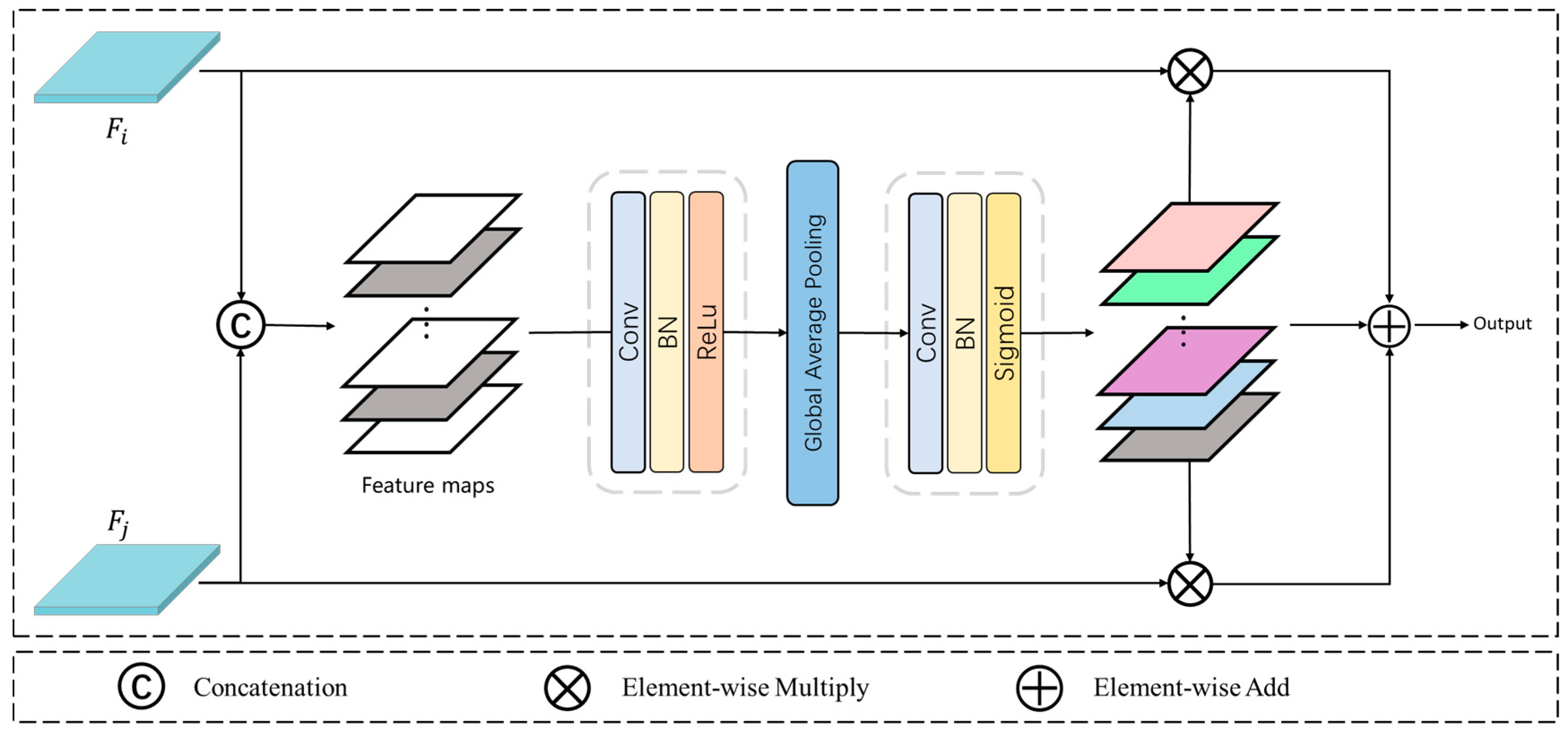
As depicted in Figure 3, the fusion process involves two feature maps of different scales ( F i and F j , i < j ). These feature maps are first concatenated along the channel dimension. Subsequently, a 1 × 1 convolution with BN and ReLU is carried out to reduce the number of channels by half. The integration of channel attention facilitates the acquisition of crucial weights, so global average pooling followed by 1 × 1 convolution and the Sigmoid function were performed to generate the feature map F m with weights, which can be calculated as follows:
F m = σ ( c 1 ( a v g ( δ ( c 1 ( c o n c a t ( F i , F j ) ) ) ) ) )
where c 1 denotes 1 × 1 convolution, concat and avg represent concatenation and global average pooling, respectively, δ and σ represent ReLU and Sigmoid functions, respectively, and F i and F j are inputs.
In this way, the generated feature map F m can serve as a weight guide for the fusion of different semantic features through multiplication. This enables the automatic learning of semantic dependencies between feature map channels. The formulation of this process can be expressed as follows:
F o u t = F i F m + F j F m
where denotes element-wise multiplication.
Finally, the SCF module hierarchically fuses the three high-level feature maps ( F 3 , F 4 , F 5 ), leading to the generation of the final fused feature map F s .
F s = S C F ( F 3 , S C F ( F 4 , F 5 ) )

3.4. Boundary-Guided Semantic Context Module

The final output of the SCF module contains rich semantic context, which can generate an initial rough water feature map, while the final output of the BR module retains salient boundary information. These two outputs complement each other in describing water bodies. Consequently, the key is to find ways to aggregate them.
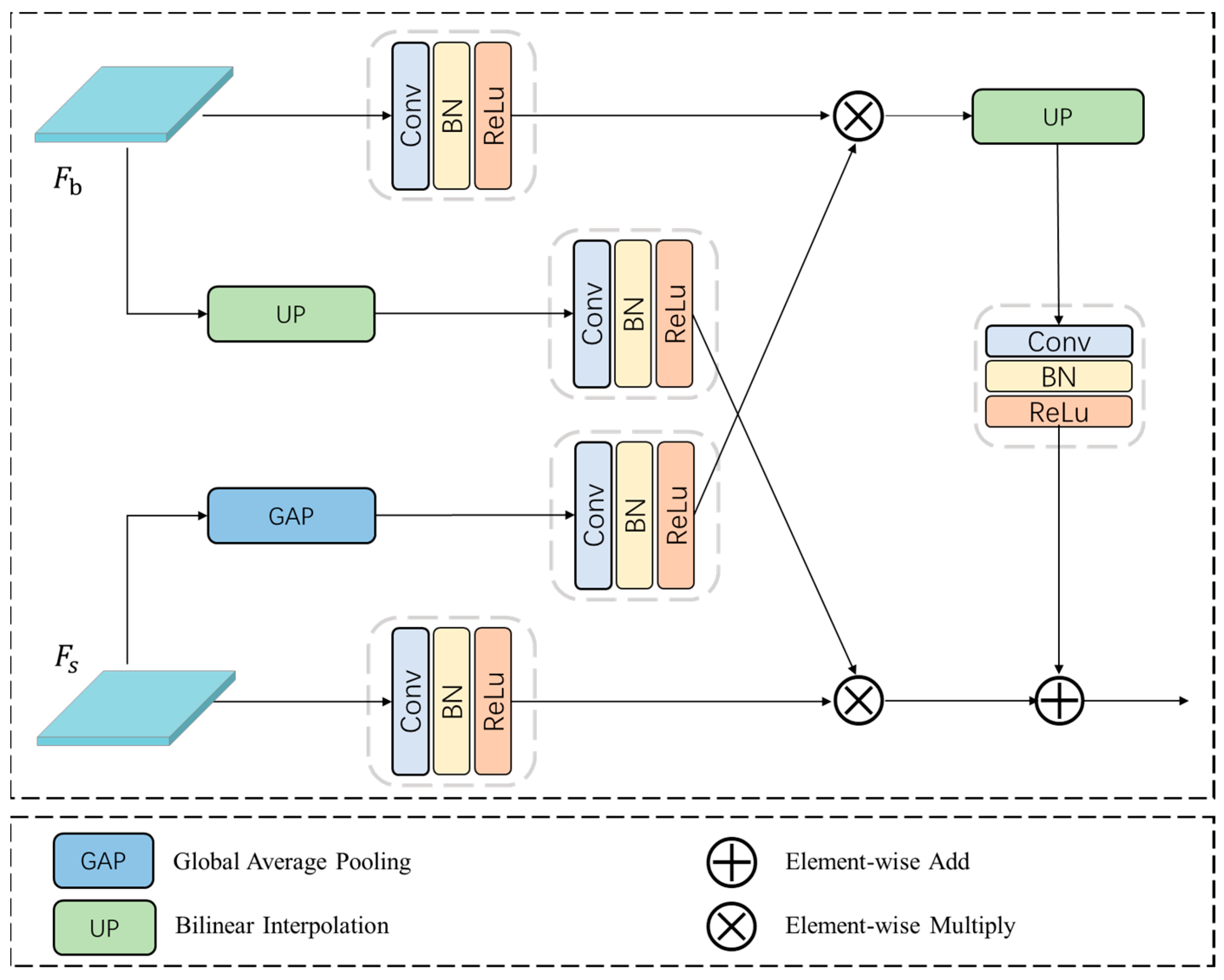
The BGS module is specifically designed to fuse boundary and semantic context. By leveraging the intrinsic partitioning capability of boundaries, BGS employs the extracted semantic boundary F b as a guide to integrate the fused semantic features F s , thereby reinforcing intra-class consistency. The BGS module adopts the method of double-branch cross-fusion, which employs details to guide the feature response of semantic context. Unlike simple compositions, this approach focuses on the hierarchical dependencies between two branches. Global average pooling is also used in the semantic branch. As such, pixels belonging to the same object exhibit a higher degree of activation in corresponding attention areas, whereas pixels from different objects demonstrate relatively fewer similarities in their activation patterns. The specific structure is shown in Figure 4.
In general, the multiplication operation serves to selectively emphasize boundary-related information, while the addition operation facilitates the complementary combination of two features. By cross-multiplying and adding, the fusion of two complementary features effectively captures the comprehensive information of an object. The process can be defined as:
F b 1 = δ ( c 3 ( F b ) )
F b 2 = δ ( c 3 ( u p ( F b ) ) )
F s 1 = δ ( c 3 ( F s ) )
F s 2 = δ ( c 3 ( a v g ( F s ) ) )
F o u t p u t = δ ( c 3 ( u p ( F b 1 F s 2 ) ) ) + F b 2 F s 1
where c 3 denotes 3 × 3 convolution, up and avg represent bilinear interpolation and global average pooling, respectively, δ represents the ReLU function, denotes element-wise multiplication, F b i and F s i are the median feature map of each branch, and F o u t p u t is the output of the BGS module.

4. Experiment

4.1. Dataset

To verify the validity and generalizability of BGSNet, a comprehensive set of experiments was conducted on the Qinghai–Tibet Plateau Lake (QTPL) [51] and the Land-cOVEr Domain Adaptive semantic segmentation (LoveDA) dataset [52].

4.1.1. The QTPL Dataset

The QTPL dataset is a collection of visible spectrum RSIs extracted from Google Earth. It consists of RGB images where only lakes are regarded as positive instances for analysis and classification. The dataset comprises a total of 6774 RSIs, all of which have a fixed size of 256 × 256. For the purpose of model training and evaluation, we randomly selected 6096 images for the training phase, while the remaining 678 images were allocated for testing.
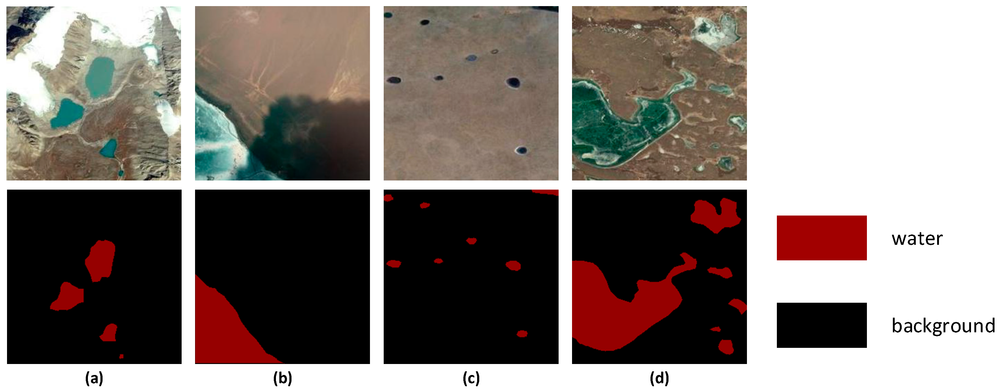
The Tibetan Plateau region has a highland lake community characterized by a concentration of salt and brackish water lakes. The genesis of the lakes is complex and varied, but most of them are developed in intermountain basins or giant valleys parallel to mountain ranges. As illustrated in Figure 5, the lakes are surrounded by complex environments, where black lakes have similar spectral characteristics to mountain and cloud shadows, and white lakes are similar to snow. In addition, the presence of discrete clusters of small water bodies adds an additional layer of challenge to achieving accurate extraction.

4.1.2. The LoveDA Dataset

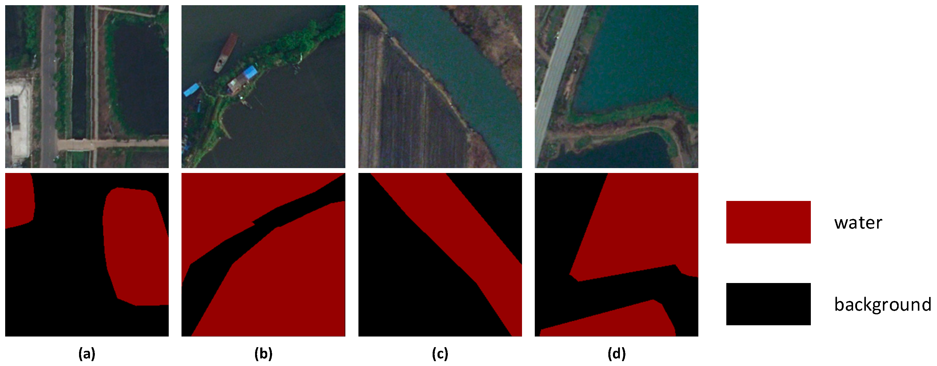
The LoveDA dataset was specifically introduced to advance research in semantic and transferable learning. The dataset contains urban and rural scenes sourced from three cities in China: Nanjing, Changzhou, and Wuhan. In urban scenes, water bodies exhibit spectral similarity to the shadows of tall buildings, which are hard to distinguish. By comparison, in rural scenarios, weeds and silt on both sides of the water body may lead to incoherent boundaries. Consequently, the accurate extraction of water bodies within heterogeneous geographical environments is challenging. Some samples are provided in Figure 6.
The LoveDA dataset contains a total of 5987 high-resolution RSIs that were collected from both urban and rural areas. To meet the requirements of the experiment, all images were cropped to a standardized size of 256 × 256 and only water in the six categories was treated as positive. Finally, a collection of 78,800 high-resolution RSIs was obtained. Similarly, these cropped images were randomly split into a training set and a test set, consisting of 63,050 and 15,750 images, respectively.

4.2. Evaluation Metrics

Water body extraction is fundamentally a semantic segmentation task. In order to assess the performance of our BGSNet, four commonly used metrics for semantic segmentation were employed: overall accuracy (OA), F1-score, mean intersection over union (MIoU), and kappa. OA is the ratio of pixels correctly classified to the total number of pixels in the image. Precision and recall assess the model’s ability to correctly identify positive samples and capture all relevant positive samples, respectively. Ideally, maximizing both metrics is desirable, but this may lead to conflict while evaluating the performance of model. To balance them, the F1-score, which is their harmonic mean, was chosen as the evaluation metric. The kappa coefficient is employed as a measure of consistency and can also gauge the effectiveness of classification. It provides insights into the agreement between labels, accounting for the possibility of agreement occurring by chance. MIoU is calculated as the average of intersection and union ratios across all categories, indicating the extent of overlap between the predicted and ground truth regions for each class. Their formulas are as follows:
O A = T P + T N T P + T N + F P + F N
F 1 - s c o r e = 2 × p r e c i s i o n × r e c a l l p r e c i s i o n + r e c a l l
p r e c i s i o n = T P T P + F P
r e c a l l = T P T P + F N
k a p p a = p 0 p e 1 p e
p 0 = O A = T P + T N T P + T N + F P + F N
p e = T P + T N × ( T P + F P ) + ( F P + F N ) × ( T N + F N ) N 2
M I o U = 1 k + 1 i = 0 k T P T P + F P + F N
where k refers to the number of all categories. T P indicates a true positive case, i.e., water pixels are correctly classified as water pixels. T N indicates a true negative case, i.e., background pixels correctly classified as background pixels. F P indicates a false positive case, i.e., background pixels are incorrectly classified as water pixels. F N indicates a false negative case, i.e., water pixels are incorrectly classified as background pixels.

4.3. Experimental Settings

The proposed BGSNet was implemented using the PyTorch deep learning framework, with Python version 3.8. All experiments were conducted on a single NVIDIA A40 GPU. During the training phase, the max epoch number of 200 was specified, and the batch size was set to 8. To optimize the network parameters, the Root Mean Square prop (RMSProp) [53] was utilized as the optimizer, with a momentum of 0.9. To facilitate the convergence of the network during training, the initial learning rate of 1 × 10⁻⁵ was set. Cross-entropy loss [54] was applied as the loss function. Its formula is as follows:
L B C E = i y i log y ^ i ( 1 y i ) log ( 1 y ^ i )
where y i and y ^ i are the true label and predicted value, respectively. Table 1 lists all hyperparameters.
We compared our approach with nine methods: UNet [24], PSPNet [26], DeeplabV3+ [27], SENet [55], Attention UNet [56], LANet [57], RAANet [58], BASNet [59], and DecoupleSegNet [60]. The settings of the above hyperparameters also apply to these methods. Notably, all comparative methods except BASNet are implemented under the same settings to enable a convincing comparison. The loss function adopted by BASNet is a novel hybrid loss function composed of cross-entropy, structural similarity, and IoU loss, which aims to emphasize the quality of water body boundaries.

4.4. Comparative Analysis

To verify the performance of the proposed BGSNet in mapping water bodies, a comparative analysis was conducted with nine advanced semantic models. These selected models represent a range of advanced techniques in semantic segmentation. UNet, PSPNet, and DeeplabV3+ are fundamental networks in the field of semantic segmentation. SENet and AttentionUNet are attention-based methods that leverage attention mechanisms to enhance intra-class consistency. BASNet uses a new hybrid loss, comprising cross-entropy, structural similarity, and IoU loss, to emphasize the quality of boundaries. DecoupleSegNet explicitly models the target object and its boundaries. Similarly, LANet and RAANet also deal with low-level details and high-level semantic information, respectively. Furthermore, to prove the generalization ability of our BGSNet, a series of experiments were conducted on the QTPL dataset and the LoveDA dataset.

4.4.1. Results on the QTPL Dataset

Table 2 reports the results of the quantitative analysis in the QTPL dataset. The performance evaluation reveals that the proposed BGSNet achieves the highest scores for OA, MIoU, F1-score, and kappa (98.97%, 97.89%,99.14%, and 0.9786, respectively). Compared with the second-best method, UNet, BGSNet improves the four metrics by 0.19%, 0.38%, 0.16%, and 0.0039, respectively, indicating that our method exhibits notable advantages in the detection of water bodies and is capable of effectively handling more complex water samples. In comparison to DeepLabV3+ and PSPNet, the well-known models for image segmentation, BGSNet demonstrates an increase in performance of at least 0.7% in OA. Attention-based methods, including Attention UNet and SENet, obtained similar results. BASNet uses the mixed loss function, but it did not perform well in the water extraction task. LANet enriches feature representation through the effective integration of features from diverse hierarchical levels, achieving 98.7% in OA. RAANet also adopts the strategy that separately deals with low-level detail information and high-level semantic information and realizes their effective fusion. Unfortunately, it failed to achieve superior results in the QTPL dataset. DecoupleSegNet decouples the body and boundary, achieving 98.84% in OA, which was second only to our approach.
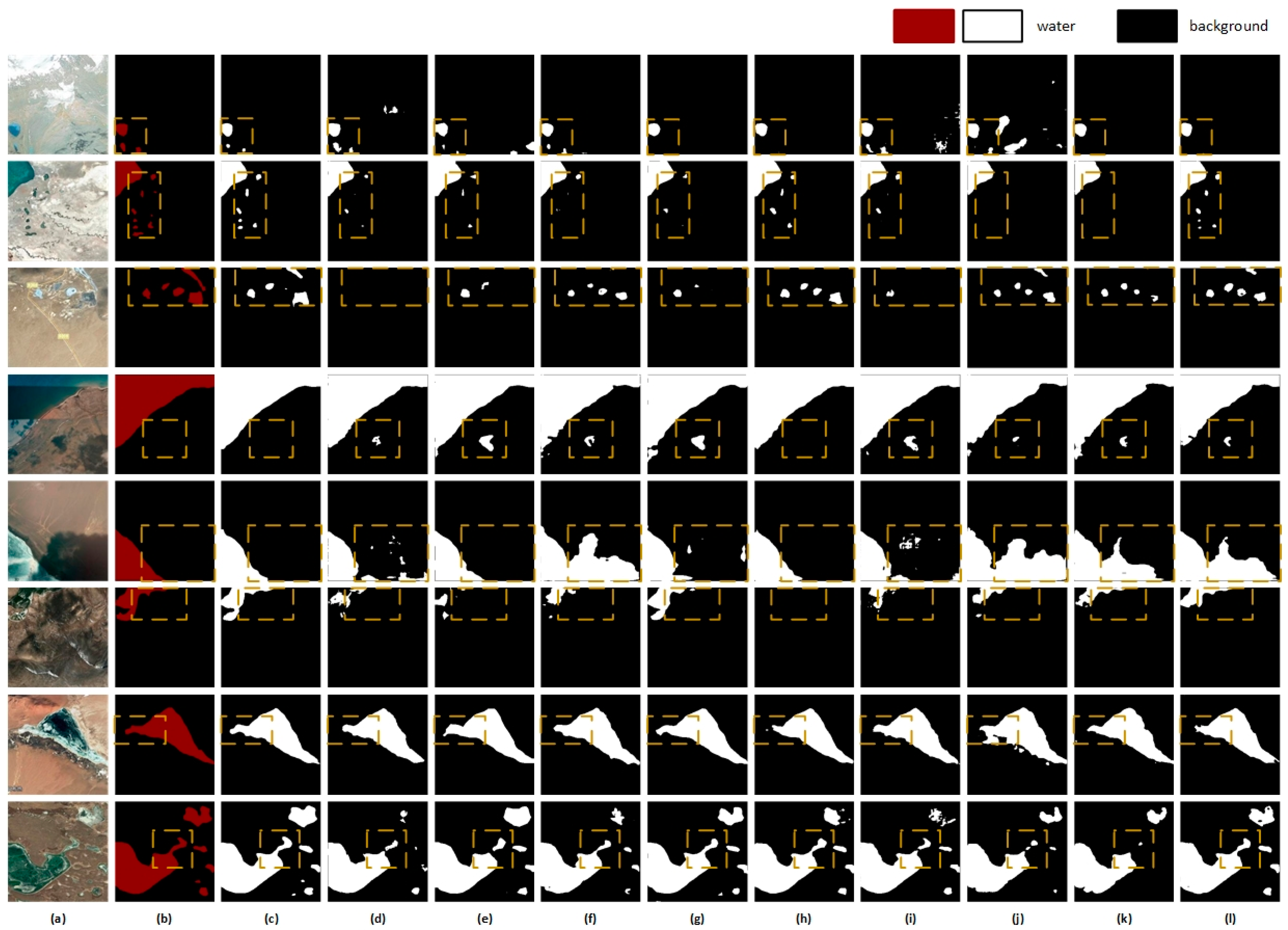
The representative results are visualized in Figure 7, where the first column shows water bodies of various sizes, shapes, and distributions. Overall, all models basically perform well in segmenting lake water bodies, but subtle differences can be observed in certain details, as indicated by the yellow boxes in the images. For relatively small and discrete water bodies (rows 1, 2), BGSNet obtains better segmentation results by using the BR module to extract shallow information to assist in localization, while other methods exhibit some degree of leakage. Similarly, for the small, narrow, and isolated water bodies in the third row, the segmentation of BGSNet is closer to the ground truth. Shadow and water often exhibit similar spectral characteristics, making them prone to misclassification. This similarity in spectral information can adversely affect the extraction accuracy. For example, in the fifth row, AttentionUNet, DeeplabV3+, PSPNet, and UNet misclassified some shadow areas as water bodies, and RAANet and BASNet misclassified almost all of the shaded parts. Compared with other methods, DecoupleSegNet can segment small water bodies (rows 1, 2, 3), but it has some difficulties in dealing with noise interference (row 5). By embedding channel attention in the SCF module, our model focuses better on water bodies with almost no misclassification. SENet and LANet, which also use the attention mechanism, perform better in distinguishing shadow areas. However, when confronted with irregularly distributed water bodies (row 6), SENet fails to describe its contour well, and LANet could not even identify the water body. BASNet specifically used the loss function to improve the quality of the boundary, but the performance here was mediocre. Since our BGS module integrates the semantic boundary and semantic context effectively, the boundary extracted by BGSNet is more complete. This can be seen from the last two lines, where BGSNet was able to completely draw the shape of irregular water bodies. Benefiting from the fact that three modules working in tandem to learn features from the whole semantic object level, our BGSNet still yields segmentation results with more complete boundaries in complicated scenarios.
The number of trainable parameters and the Flops (floating point operations) are listed in Table 3. It is worth noting that BGSNet has half the computational complexity of the multi-scale networks DeeplabV3+ and PSPNet. The quantitative results of DecoupleSegNet are second only to our method, but the computational complexity is much higher than ours. SENet possesses the fewest parameters, while the proposed BGSNet does not increase much but performs better, achieving a balance of accuracy and efficiency.

4.4.2. Results on the LoveDA dataset

The proposed BGSNet was further evaluated by conducting the same experiment on the LoveDA dataset to validate its performance. Consistent with the results of the QTPL dataset, BGSNet still achieved the highest scores (95.70%, 80.86%, 97.59%, and 0.7745, respectively) for all evaluation metrics in Table 4. In comparison to other methods, BGSNet demonstrated superior improvements across all indicators.
Figure 8 displays some samples for the LoveDA datasets. Compared with other models, prediction results of BGSNet are closer to the real situation. Similarly, all models can segment large areas of water bodies, but the boundary extracted by BGSNet and SENet is obviously smoother and more detailed (rows 1, 2). However, for areas with shadow interference (row 3) and multiple adjacent water bodies (row 4), SENet fails to yield improved results despite its inclusion of an attention mechanism, while, due to the accurate localization of the BR module and the focusing of the SCF module, BGSNet significantly outperforms the other methods according to the segmentation results. LANet also integrates shallow spatial information to facilitate water body localization, but the processing at the boundary area is not satisfactory. RAANet and DecoupleSegNet struggle to effectively distinguish the regions with similar spectral characteristics from water bodies (rows 3, 5). Similarly, BASNet was able to identify most water bodies, but the segmentation of easily confused areas was unsatisfactory (rows 3, 5 6). PSPNet and Deeplabv3+ proved more suitable for processing large areas of water bodies (rows 2, 8). By integrating three modules, BGSNet can achieve accurate segmentation results within intricate and challenging scenarios.

4.5. Ablation Analysis

In order to suppress the noise interference, the highest-level feature map was used to obtain semantic boundaries in the boundary extraction stage. Therefore, the ablation study was first performed to ascertain the efficacy and indispensability of the fusion of feature map F 5 . Two low-level feature maps F 1 and F 2 were fixed, and then fused as F 3 , F 4 , and F 5 respectively. The results can be seen in Table 5. Fusion ( F 1 , F 2 , F 5 ) is the proposed BGSNet. Compared with F 4 , F 3 , and no fusion, fusion F 5 can achieve the best segmentation accuracy. In particular, in the LoveDA dataset, the reduction is more obvious. Although the number of parameters decreased by 0.074 when only using F 1 and F 2 , the OA, MIoU, F1-score, and kappa decreased by 0.11%, 0.22%, 0.09%, and 0.0021, respectively on the QTPL dataset and 0.33%, 1.61%, 0.17%, and 0.0266 on the LoveDA dataset. We suggest that it is acceptable to sacrifice time for significant improvements.
Further, to evaluate the effectiveness of the three involved modules, the ablation study was also performed on two datasets. The quantitative results are presented in Table 6, illustrating the positive impact exhibited by all three modules in enhancing the performance of the model across both datasets. A more noticeable difference in accuracy was also observed in the LoveDA dataset. For the LoveDA dataset, after removing BE, the OA, MIoU, F1-score, and kappa decreased by 0.45%, 1.98%, 0.25%, and 0.028, respectively. After removing SCF, the corresponding decreases were 0.64%, 2.6%, 0.35%, and 0.0369, respectively. Similarly, when BGS was removed, the decreases were 1.42%, 5.47%, 0.78%, and 0.0798, respectively. It can also be determined from the downward trend that the BGS module made a greater contribution to improving accuracy. Regarding the parameters, an increase of 0.222 M was deemed acceptable.
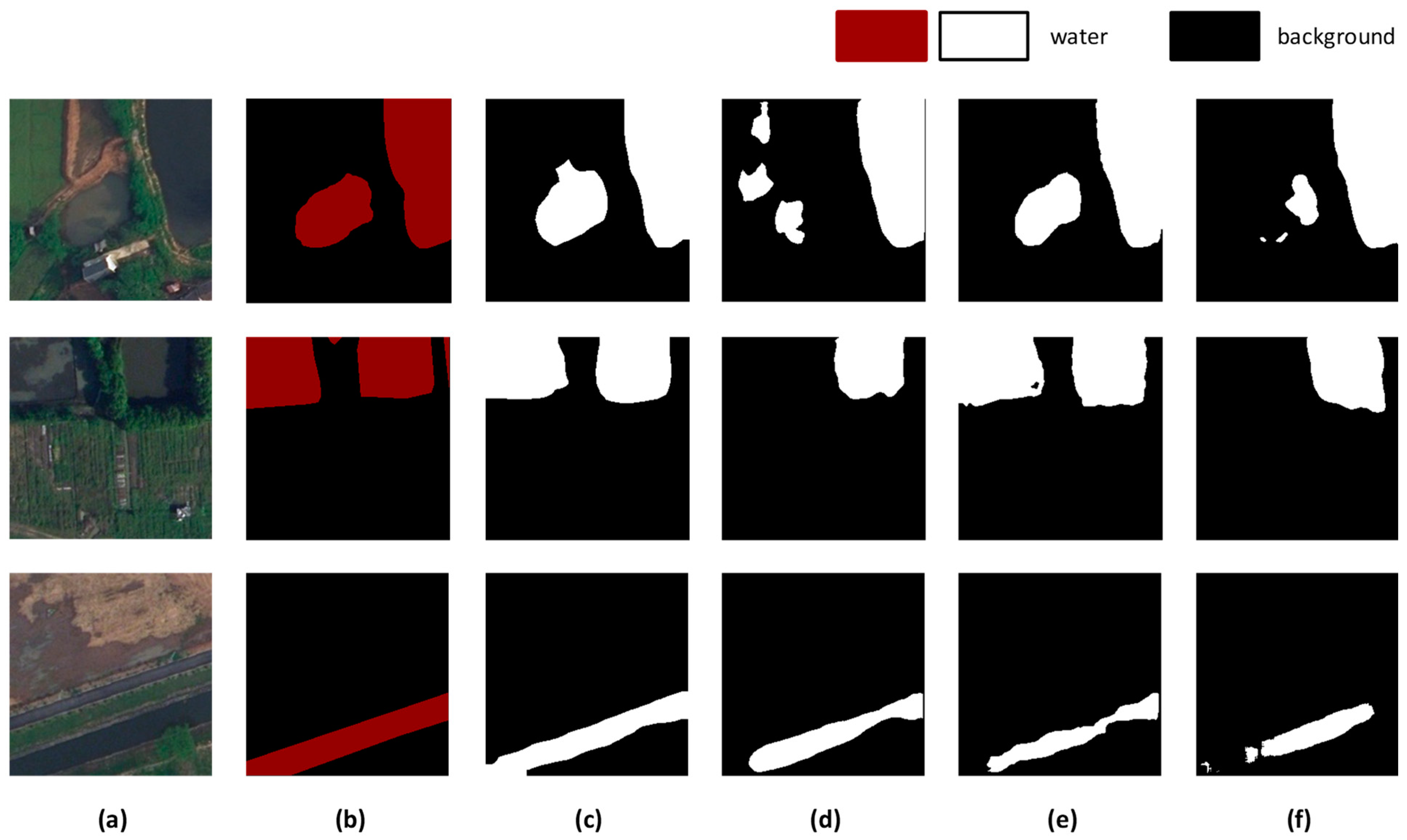
Figure 8 and Figure 9 depict the visualizations of the ablation study. The visualization results revealed that when three modules are removed separately, some tiny water bodies are missing (Figure 9 row 2). After removing BR, water bodies covered by the shadow (Figure 9 row 3) and similar to the background (Figure 10 rows 1, 2) were misclassified as background. Likewise, when SCF was removed, it also misclassified water bodies as background, but it can correctly classify water in complex scenarios (Figure 10 rows 1, 2).

5. Conclusions

In this paper, we propose a boundary-guided semantic context network (BGSNet) to accurately segment water bodies from RSIs. Striving to bridge boundary representations and semantic context, three specific modules are designed:
(1)
The BR module is designed to obtain prominent boundary information which is beneficial for localization.
(2)
The SCF module is embedded to capture semantic context for generating a coarse feature map.
(3)
The BGS module is devised to aggregate context information along the boundaries, facilitating the mutual enhancement of internal pixels belonging to the same class, thereby improving intra-class consistency.
Extensive experiments were conducted on the QTPL and the LoveDA datasets, demonstrating the superiority of the proposed method compared to existing mainstream methods.
With the advancements of aeronautics and space technology, a large number of detailed remote sensing images have been captured. Due to the influences of imaging conditions and water quality, the distinctiveness among water bodies has been progressively amplified. Furthermore, due to the presence of silt along riverbanks and the blurred shadows cast by towering vegetation, there is increasing resemblance between water bodies and their surrounding environments. These factors pose a further challenge to the extraction of water bodies. In future, our endeavors will focus on model refinement to adapt to these demanding scenarios.

Author Contributions

Conceptualization, X.L. (Xin Lyu) and J.Y.; methodology, J.Y.; software, W.J.; validation, X.L. (Xin Lyu) and Z.X.; formal analysis, X.L. (Xin Li); investigation, X.W. and X.L. (Xin Li); resources, Y.C., X.L. (Xin Lyu) and X.L. (Xin Li); data curation, Y.C. and Y.F.; writing—original draft preparation, J.Y.; writing—review and editing, X.L. (Xin Lyu), J.Y. and X.L. (Xin Li); visualization, X.L. (Xin Lyu) and J.Y.; supervision, Y.C., X.L. (Xin Lyu) and X.L. (Xin Li); project administration, Y.C. and X.L. (Xin Lyu); funding acquisition, Y.C and X.L. (Xin Lyu). All authors have read and agreed to the published version of the manuscript.

Funding

This research was funded by the High Resolution Earth Observing System-Water Application Demonstration (Grant No. 08-Y30F02-9001-20/22), the Excellent Post-doctoral Program of Jiangsu Province (Grant No. 2022ZB166), the Fundamental Research Funds for the Central Universities (Grant No. B230201007), the Project of Water Science and Technology of Jiangsu Province (Grant No. 2021080), the National Natural Science Foundation of China (Grant No. 42104033, 42101343).

Institutional Review Board Statement

Not applicable.

Informed Consent Statement

Not applicable.

Data Availability Statement

The datasets in our study are public. The Qinghai–Tibet Plateau Lake dataset can be found at http://www.ncdc.ac.cn/portal/metadata/b4d9fb27-ec93-433d-893a-2689379a3fc0, (accessed on 16 March 2023). The Land-cOVEr Domain Adaptive semantic segmentation dataset can be found at https://drive.google.com/drive/folders/1ibYV0qwn4yuuh068Rnc-w4tPi0U0c-ti, (accessed on 16 March 2023).

Conflicts of Interest

The authors declare no conflict of interest.

References

  1. Oki, T.; Kanae, S. Global hydrological cycles and world water resources. Science 2006, 313, 1068–1072. [Google Scholar] [CrossRef] [PubMed]
  2. Liu, H.; Zheng, L.; Jiang, L.; Liao, M. Forty-Year Water Body Changes in Poyang Lake and the Ecological Impacts Based on Landsat and HJ-1 A/B Observations. J. Hydrol. 2020, 589, 125161. [Google Scholar] [CrossRef]
  3. Xu, N.; Gong, P. Significant Coastline Changes in China during 1991–2015 Tracked by Landsat Data. Sci. Bull. 2018, 63, 883–886. [Google Scholar] [CrossRef] [PubMed]
  4. Chen, Y.; Fan, R.; Yang, X.; Wang, J.; Latif, A. Extraction of urban water bodies from high-resolution remote-sensing imagery using deep learning. Water 2018, 10, 585. [Google Scholar] [CrossRef]
  5. Xu, N.; Ma, Y.; Zhang, W.; Wang, X.H. Surface-Water-Level Changes During 2003–2019 in Australia Revealed by ICESat/ICESat-2 Altimetry and Landsat Imagery. IEEE Geosci. Remote Sens. Lett. 2021, 18, 1129–1133. [Google Scholar] [CrossRef]
  6. Ovando, A.; Martinez, J.M.; Tomasella, J.; Rodriguez, D.A.; von Randow, C. Multi temporal flood mapping and satellite altimetry used to evaluate the flood dynamics of the Bolivian Amazon wetlands. Int. J. Appl. Earth Obs. Geoinf. 2018, 69, 27–40. [Google Scholar] [CrossRef]
  7. Ma, Y.; Xu, N.; Sun, J.; Wang, X.H.; Yang, F.; Li, S. Estimating Water Levels and Volumes of Lakes Dated Back to the 1980s Using Landsat Imagery and Photon-Counting Lidar Datasets. Remote Sens. Environ. 2019, 232, 111287. [Google Scholar] [CrossRef]
  8. Li, R.; Liu, W.; Yang, L.; Sun, S.; Hu, W.; Zhang, F.; Li, W. DeepUNet: A Deep Fully Convolutional Network for Pixel-Level Sea-Land Segmentation. IEEE J. Sel. Top. Appl. Earth Obs. Remote Sens. 2018, 11, 3954–3962. [Google Scholar] [CrossRef]
  9. Ji, L.; Gong, P.; Wang, J.; Shi, J.; Zhu, Z. Construction of the 500-m Resolution Daily Global Surface Water Change Database (2001–2016). Water Resour. Res. 2018, 54, 10270–10292. [Google Scholar] [CrossRef]
  10. Li, X.; Xu, F.; Xia, R.; Lyu, X.; Gao, H.; Tong, Y. Hybridizing Cross-Level Contextual and Attentive Representations for Remote Sensing Imagery Semantic Segmentation. Remote Sens. 2021, 13, 2986. [Google Scholar] [CrossRef]
  11. Hamm NA, S.; Atkinson, P.M.; Milton, E.J. A per-pixel, non-stationary mixed model for empirical line atmospheric correction in remote sensing. Remote Sens. Environ. 2012, 124, 666–678. [Google Scholar] [CrossRef]
  12. Li, Y.; Dang, B.; Zhang, Y.; Du, Z. Water body classification from high-resolution optical remote sensing imagery: Achievements and perspectives. ISPRS J. Photogramm. Remote Sens. 2022, 187, 306–327. [Google Scholar] [CrossRef]
  13. Xie, H.; Luo, X.; Xu, X.; Tong, X.; Jin, Y.; Pan, H.; Zhou, B. New hyperspectral difference water index for the extraction of urban water bodies by the use of airborne hyperspectral images. J. Appl. Remote Sens. 2014, 8, 085098. [Google Scholar] [CrossRef]
  14. McFeeters, S.K. The use of the Normalized Difference Water Index (NDWI) in the delineation of open water features. Int. J. Remote Sens. 1996, 17, 1425–1432. [Google Scholar] [CrossRef]
  15. Xu, H. Modification of normalised difference water index (NDWI) to enhance open water features in remotely sensed imagery. Int. J. Remote Sens. 2006, 27, 3025–3033. [Google Scholar] [CrossRef]
  16. Ji, L.; Zhang, L.; Wylie, B. Analysis of dynamic thresholds for the normalized difference water index. Photogramm. Eng. Remote Sens. 2009, 75, 1307–1317. [Google Scholar] [CrossRef]
  17. Feyisa, G.L.; Meilby, H.; Fensholt, R.; Proud, S.R. Automated Water Extraction Index: A new technique for surface water mapping using Landsat imagery. Remote Sens. Environ. 2014, 140, 23–35. [Google Scholar] [CrossRef]
  18. Guo, H.; He, G.; Jiang, W.; Yin, R.; Yan, L.; Leng, W. A Multi-Scale Water Extraction Convolutional Neural Network (MWEN) Method for GaoFen-1 Remote Sensing Images. ISPRS Int. J. Geo-Inf. 2020, 9, 189. [Google Scholar] [CrossRef]
  19. Hinton, G.E.; Osindero, S.; Teh, Y.W. A fast learning algorithm for deep belief nets. Neural Comput. 2006, 18, 1527–1554. [Google Scholar] [CrossRef]
  20. He, K.M.; Zhang, X.Y.; Ren, S.Q.; Sun, J. Deep residual learning for image recognition. In Proceedings of the 2016 IEEE Conference on Computer Vision and Pattern Recognition (CVPR), Las Vegas, NV, USA, 26 June–1 July 2016; pp. 770–778. [Google Scholar]
  21. Li, X.; Xu, F.; Xia, R.; Li, T.; Chen, Z.; Wang, X.; Xu, Z.; Lyu, X. Encoding Contextual Information by Interlacing Transformer and Convolution for Remote Sensing Imagery Semantic Segmentation. Remote Sens. 2022, 14, 4065. [Google Scholar] [CrossRef]
  22. Ming, Q.; Miao, L.; Zhou, Z.; Dong, Y. Cfc-net: A critical feature capturing network for arbitrary-oriented object detection in remote sensing images. arXiv 2021, arXiv:2101.06849. [Google Scholar] [CrossRef]
  23. Long, J.; Shelhamer, E.; Darrell, T. Fully Convolutional Networks for Semantic Segmentation. IEEE Trans. Pattern Anal. Mach. Intell. 2015, 39, 640–651. [Google Scholar] [CrossRef]
  24. Ronneberger, O.; Fischer, P.; Brox, T. U-net: Convolutional networks for biomedical image segmentation. In Proceedings of the International Conference on Medical Image Computing and Computer-Assisted Intervention (MICCAI), Munich, Germany, 5–9 October 2015; pp. 234–241. [Google Scholar]
  25. Badrinarayanan, V.; Kendall, A.; Cipolla, R. Segnet: A deep convolutional encoder-decoder architecture for image segmentation. IEEE Trans. Pattern Anal. Mach. Intell. 2017, 39, 2481–2495. [Google Scholar] [CrossRef]
  26. Zhao, H.; Shi, J.; Qi, X.; Wang, X.; Jia, J. Pyramid Scene Parsing Network. In Proceedings of the IEEE Conference on Computer Vision and Pattern Recognition (CVPR), Honolulu, HI, USA, 21–26 July 2017; pp. 6230–6239. [Google Scholar]
  27. Chen, L.; Zhu, Y.; Papandreou, G.; Schroff, F.; Adam, H. Encoder-decoder with atrous separable convolution for semantic image segmentation. In Proceedings of the European Conference on Computer Vision (ECCV), Munich, Germany, 8–14 September 2018; pp. 801–818. [Google Scholar]
  28. Miao, Z.; Fu, K.; Sun, H.; Sun, X.; Yan, M. Automatic water-body segmentation from high-resolution satellite images via deep networks. IEEE Geosci. Remote Sens. Lett. 2018, 15, 602–606. [Google Scholar] [CrossRef]
  29. Feng, W.; Sui, H.; Huang, W.; Xu, C.; An, K. Water Body Extraction from Very High-Resolution Remote Sensing Imagery Using Deep U-Net and a Superpixel-Based Conditional Random Field Model. IEEE Geosci. Remote Sens. Lett. 2019, 16, 618–622. [Google Scholar] [CrossRef]
  30. Wang, Y.; Li, Z.; Zeng, C.; Xia, G.-S.; Shen, H. An Urban Water Extraction Method Combining Deep Learning and Google Earth Engine. IEEE J. Sel. Top. Appl. Earth Obs. Remote Sens. 2020, 13, 769–782. [Google Scholar] [CrossRef]
  31. Qin, P.; Cai, Y.; Wang, X. Small Waterbody Extraction with Improved U-Net Using Zhuhai-1 Hyperspectral Remote Sensing Images. IEEE Geosci. Remote Sensing Lett. 2022, 19, 5502705. [Google Scholar] [CrossRef]
  32. Li, X.; Xu, F.; Liu, F.; Xia, R.; Tong, Y.; Li, L.; Xu, Z.; Lyu, X. Hybridizing Euclidean and Hyperbolic Similarities for Attentively Refining Representations in Semantic Segmentation of Remote Sensing Images. IEEE Geosci. Remote Sensing Lett. 2022, 19, 5003605. [Google Scholar] [CrossRef]
  33. Li, X.; Xu, F.; Liu, F.; Lyu, X.; Tong, Y.; Xu, Z.; Zhou, J. A Synergistical Attention Model for Semantic Segmentation of Remote Sensing Images. IEEE Trans. Geosci. Remote Sensing. 2023, 61, 5400916. [Google Scholar] [CrossRef]
  34. He, J.; Deng, Z.; Zhou, L.; Wang, Y.; Qiao, Y. Adaptive pyramid context network for semantic segmentation. In Proceedings of the IEEE/CVF Conference on Computer Vision and Pattern Recognition, Long Beach, CA, USA, 15–20 June 2019; pp. 7519–7528. [Google Scholar]
  35. Ma, B.; Chang, C. Semantic Segmentation of High-Resolution Remote Sensing Images Using Multiscale Skip Connection Network. IEEE Sens. J. 2022, 22, 3745–3755. [Google Scholar] [CrossRef]
  36. Li, X.; Xu, F.; Lyu, X.; Gao, H.; Tong, Y.; Cai, S.; Li, S.; Liu, D. Dual Attention Deep Fusion Semantic Segmentation Networks of Large-Scale Satellite Remote-Sensing Images. Int. J. Remote Sens. 2021, 42, 3583–3610. [Google Scholar] [CrossRef]
  37. Li, R.; Zheng, S.; Zhang, C.; Duan, C.; Su, J.; Wang, L.; Atkinson, P.M. Multiattention Network for Semantic Segmentation of Fine-Resolution Remote Sensing Images. IEEE Trans. Geosci. Remote Sens. 2022, 60, 5607713. [Google Scholar] [CrossRef]
  38. Nong, Z.; Su, X.; Liu, Y.; Zhan, Z.; Yuan, Q. Boundary-Aware Dual-Stream Network for VHR Remote Sensing Images Semantic Segmentation. IEEE J. Sel. Top. Appl. Earth Obs. Remote Sens. 2021, 14, 5260–5268. [Google Scholar] [CrossRef]
  39. Li, X.; Li, T.; Chen, Z.; Zhang, K.; Xia, R. Attentively Learning Edge Distributions for Semantic Segmentation of Remote Sensing Imagery. Remote Sens. 2022, 14, 102. [Google Scholar] [CrossRef]
  40. Bokhovkin, A.; Burnaev, E. Boundary loss for remote sensing imagery semantic segmentation. In International Symposium on Neural Networks; Springer: Cham, Switzerland, 2019; pp. 388–401. [Google Scholar]
  41. Yu, Y.; Huang, L.; Lu, W.; Guan, H.; Ma, L.; Jin, S.; Yu, C.; Zhang, Y.; Tang, P.; Liu, Z.; et al. WaterHRNet: A multibranch hierarchical attentive network for water body extraction with remote sensing images. Int. J. Appl. Earth Obs. Geoinf. 2022, 115, 103103. [Google Scholar] [CrossRef]
  42. Kang, J.; Guan, H.; Peng, D.; Chen, Z. Multi-scale context extractor network for water-body extraction from high-resolution optical remotely sensed images. Int. J. Appl. Earth Obs. Geoinf. 2021, 103, 102499. [Google Scholar] [CrossRef]
  43. Xia, M.; Cui, Y.; Zhang, Y.; Xu, Y.; Liu, J.; Xu, Y. DAU-Net: A novel water areas segmentation structure for remote sensing image. Int. J. Remote Sens. 2021, 42, 2594–2621. [Google Scholar] [CrossRef]
  44. Zhang, X.; Li, J.; Hua, Z. MRSE-Net: Multiscale Residuals and SE-Attention Network for Water Body Segmentation from Satellite Images. IEEE J. Sel. Top. Appl. Earth Obs. Remote Sens. 2022, 15, 5049–5064. [Google Scholar] [CrossRef]
  45. Yu, Y.; Yao, Y.; Guan, H.; Li, D.; Liu, Z.; Wang, L.; Yu, C.; Xiao, S.; Wang, W.; Chang, L. A self-attention capsule feature pyramid network for water body extraction from remote sensing imagery. Int. J. Remote Sens. 2021, 42, 1801–1822. [Google Scholar] [CrossRef]
  46. Krahenbühl, P.; Koltun, V. Efficient inference in fully connected crfs with gaussian edge potentials. arXiv 2011, arXiv:1210.5644. [Google Scholar]
  47. Chu, Z.; Tian, T.; Feng, R.; Wang, L. Sea-Land Segmentation with Res-UNet and Fully Connected CRF. In Proceedings of the IGARSS 2019—2019 IEEE International Geoscience and Remote Sensing Symposium, Yokohama, Japan, 28 July–2 August 2019; pp. 3840–3843. [Google Scholar]
  48. Jin, Y.; Xu, W.; Zhang, C.; Luo, X.; Jia, H. Boundary-aware refined network for automatic building extraction in very high-resolution urban aerial images. Remote Sens. 2021, 13, 692. [Google Scholar] [CrossRef]
  49. Zhang, Z.; Lu, M.; Ji, S.; Yu, H.; Nie, C. Rich CNN Features for Water-Body Segmentation from Very High Resolution Aerial and Satellite Imagery. Remote Sens. 2021, 13, 1912. [Google Scholar] [CrossRef]
  50. Wang, B.; Chen, Z.; Wu, L.; Yang, X.; Zhou, Y. SADA-Net: A Shape Feature Optimization and Multiscale Context Information Based Water Body Extraction Method for High-Resolution Remote Sensing Images. IEEE J. Sel. Top. Appl. Earth Obs. Remote Sens. 2022, 15, 1744–1759. [Google Scholar] [CrossRef]
  51. Wang, Z.; Gao, X.; Zhang, Y.; Zhao, G. MSLWENet: A Novel Deep Learning Network for Lake Water Body Extraction of Google Remote Sensing Images. Remote Sens. 2020, 12, 4140. [Google Scholar] [CrossRef]
  52. Wang, J.; Zheng, Z.; Ma, A.; Lu, X.; Zhong, Y. LoveDA: A Remote Sensing Land-Cover Dataset for Domain Adaptive Semantic Segmentation. arXiv 2021, arXiv:2110.08733. [Google Scholar]
  53. Ruder, S. An Overview of Gradient Descent Optimization Algorithms. arXiv 2017, arXiv:1609.04747. [Google Scholar]
  54. De Boer, P.T.; Kroese, D.P.; Mannor, S. A Tutorial on the Cross-Entropy Method. Ann. Oper. Res. 2005, 134, 19–67. [Google Scholar] [CrossRef]
  55. Hu, J.; Shen, L.; Sun, G. Squeeze-and-Excitation Networks. In Proceedings of the 2018 IEEE/CVF Conference on Computer Vision and Pattern Recognition, Salt Lake City, UT, USA, 18–23 June 2018; pp. 7132–7141. [Google Scholar]
  56. Schlemper, J.; Oktay, O.; Schaap, M.; Heinrich, M.; Kainz, B.; Glocker, B.; Rueckert, D. Attention gated networks: Learning to leverage salient regions in medical images. Med. Image Anal. 2019, 53, 197–207. [Google Scholar] [CrossRef] [PubMed]
  57. Ding, L.; Tang, H.; Bruzzone, L. LANet: Local Attention Embedding to Improve the Semantic Segmentation of Remote Sensing Images. IEEE Trans. Geosci. Remote Sens. 2021, 59, 426–435. [Google Scholar] [CrossRef]
  58. Liu, R.; Tao, F.; Liu, X.; Na, J.; Leng, H.; Wu, J.; Zhou, T. RAANet: A Residual ASPP with Attention Framework for Semantic Segmentation of High-Resolution Remote Sensing Images. Remote Sens. 2022, 14, 3109. [Google Scholar] [CrossRef]
  59. Qin, X.; Fan, D.; Huang, C.; Diagne, C.; Zhang, Z. Boundary-Aware Segmentation Network for Mobile and Web Applications. arXiv 2021, arXiv:2101.04704. [Google Scholar]
  60. Li, X.; Li, X.; Li, Z.; Cheng, G.; Shi, J.; Lin, Z.; Tan, S.; Tong, Y. Improving Semantic Segmentation via Decoupled Body and Edge Supervision. arXiv 2020, arXiv:2007.10035. [Google Scholar]
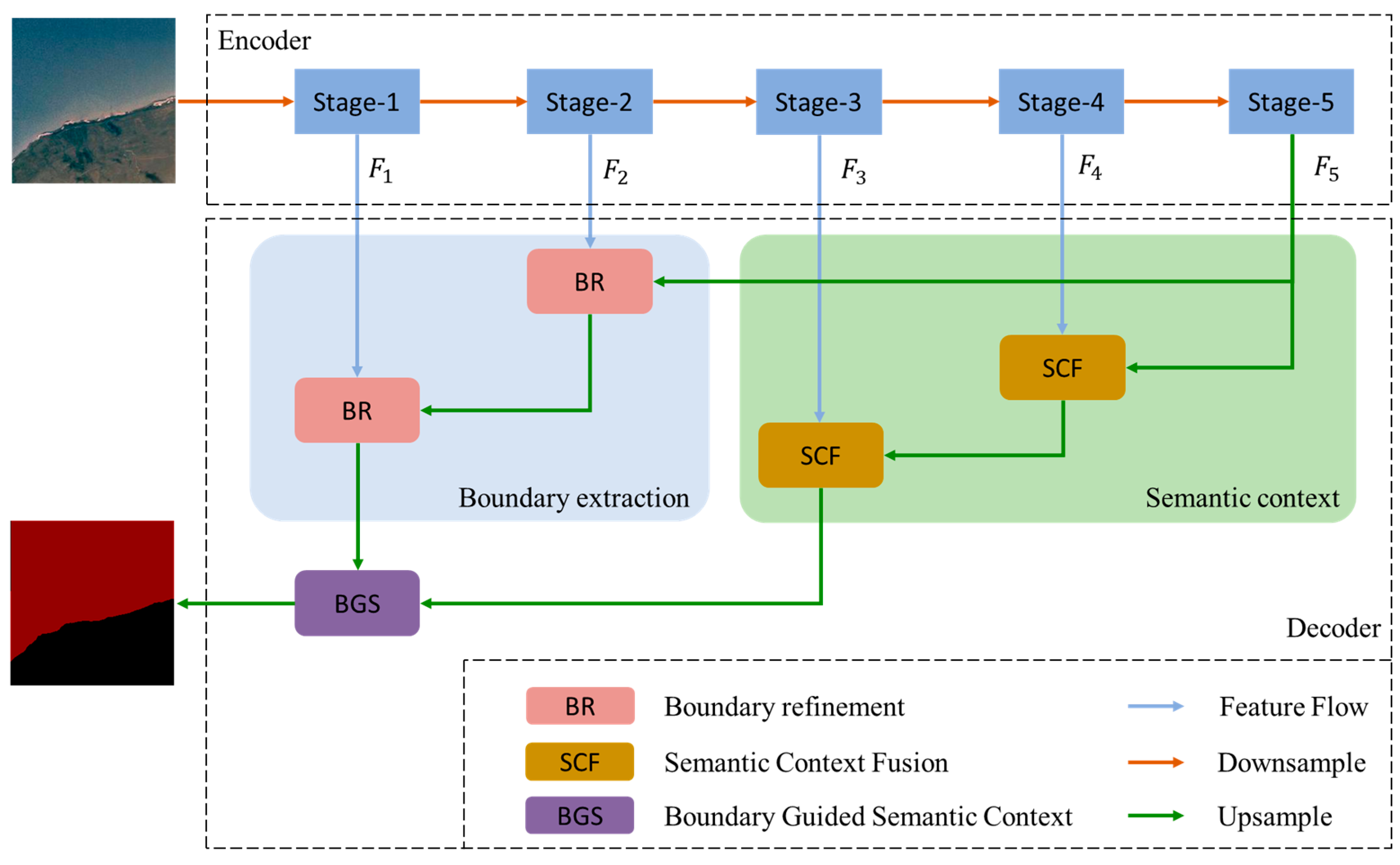
Figure 1. The structure of the proposed BGSNet.
Remotesensing 15 04325 g001
Figure 2. The boundary refinement (BR) module.
Remotesensing 15 04325 g002
Figure 3. The semantic context fusion (SCF) module.
Remotesensing 15 04325 g003
Figure 4. The BGS module.
Remotesensing 15 04325 g004
Figure 5. Some samples on the QTPL dataset. The first row is the remote sensing image, and the second row is the labeled image.
Remotesensing 15 04325 g005
Figure 6. Some samples on the LoveDA dataset. The first row is the remote sensing image, and the second row is the labeled image.
Remotesensing 15 04325 g006
Figure 7. Visualizations on the QTPL dataset: (a) image, (b) ground truth, (c) proposed BGSNet, (d) Attention UNet, (e) SENet, (f) Deeplabv3+, (g) PSPNet, (h) LANet, (i) UNet, (j) RAANet, (k) BASNet, (l) DecoupleSegNet. The yellow boxes indicate obvious differences.
Remotesensing 15 04325 g007
Figure 8. Visualizations on the LoveDA dataset: (a) image, (b) ground truth, (c) proposed BGSNet, (d) Attention UNet, (e) SENet, (f) Deeplabv3+, (g) PSPNet, (h) LANet, (i) UNet, (j) RAANet, (k) BASNet, (l) DecoupleSegNet. The yellow boxes indicate obvious differences.
Remotesensing 15 04325 g008
Figure 9. Visualizations of ablation study on the QTPL dataset: (a) image, (b) ground truth, (c) BGSNet, (d) BGSNet without BR, (e) BGSNet without SCF, (f) BGSNet without BGS.
Remotesensing 15 04325 g009
Figure 10. Visualizations of ablation study on the LoveDA dataset: (a) image, (b) ground truth, (c) BGSNet, (d) BGSNet without BR, (e) BGSNet without SCF, (f) BGSNet without BGS.
Remotesensing 15 04325 g010
Table 1. Hyperparameter settings.
ItemsSettings
Max epoch200
Batch Size8
OptimizerRMSProp
Momentum0.9
Initial learning rate1 × 10−5
Loss functionCross-entropy loss
Table 2. Quantitative results on the QTPL dataset.
MethodOA (%)MIoU (%)F1-ScoreKappa
RAANet97.4894.9297.890.9478
BASNet98.8697.1498.820.9709
DecoupleSegNet98.8997.3798.920.9733
DeeplabV3+98.2796.4898.540.9642
PSPNet98.7497.4398.950.9740
LANet98.7397.4098.930.9737
Attention UNet98.6797.2998.880.9725
SENet98.6597.2498.860.9720
UNet98.7897.5198.980.9747
BGSNet98.9797.8999.140.9786
Table 3. Comparison results for model complexity and training Flops. The input size is 3 × 256 × 256.
MethodsParams (M)Flops (G)
RAANet64.204186.201
BASNet87.0801021.531
DecoupleSegNet137.1001457.126
DeeplabV3+54.608166.053
PSPNet46.707368.898
LANet23.79266.475
Attention UNet34.87966.636
SENet23.77565.93
UNet34.527524.179
BGSNet24.22179.596
Table 4. Quantitative results on the LoveDA dataset.
MethodOA (%)MIoU (%)F1-ScoreKappa
RAANet93.1171.6996.150.6359
BASNet93.0771.8696.450.6382
DecoupleSegNet94.9575.9995.120.6366
DeeplabV3+92.4571.8495.710.5867
PSPNet93.4173.3696.300.6634
LANet95.4779.7197.470.7583
Attention UNet94.2773.9296.830.6715
SENet95.0178.8497.190.7463
UNet94.6275.9597.010.7032
BGSNet95.7080.8697.590.7745
Table 5. Quantitative results of different inputs on two datasets. Fusion ( F 1 , F 2 , F 5 ) is proposed BGSNet.
DatasetMethodsOA (%)MIoU (%)F1-ScoreKappaParams (M)
QTPLFusion ( F 1 , F 2 )98.8697.6799.050.976524.147
Fusion ( F 1 , F 2 , F 3 )98.9397.8199.100.977824.221
Fusion ( F 1 , F 2 , F 4 )98.9697.8699.120.978424.221
Fusion ( F 1 , F 2 , F 5 )98.9797.8999.140.978624.221
LoveDAFusion ( F 1 , F 2 )95.3779.2597.420.751924.147
Fusion ( F 1 , F 2 , F 3 )95.4780.0597.460.763324.221
Fusion ( F 1 , F 2 , F 4 )95.3679.6997.400.758224.221
Fusion ( F 1 , F 2 , F 5 )95.7080.8697.590.774524.221
Table 6. Quantitative results of ablation study on two datasets.
DatasetMethodsOA (%)MIoU (%)F1-ScoreKappaParams (M)
QTPLBGSNet98.9797.8999.140.978624.221
BGSNet (without BR)98.8997.7299.060.976924.073
BGSNet (without SCF)98.8797.6899.050.976524.131
BGSNet (without BGS)98.8297.5999.010.975623.999
LoveDABGSNet95.7080.8697.590.774524.221
BGSNet (without BR)95.2578.8897.340.746524.073
BGSNet (without SCF)95.0678.2697.240.737624.131
BGSNet (without BGS)94.2875.3996.810.694723.999
Disclaimer/Publisher’s Note: The statements, opinions and data contained in all publications are solely those of the individual author(s) and contributor(s) and not of MDPI and/or the editor(s). MDPI and/or the editor(s) disclaim responsibility for any injury to people or property resulting from any ideas, methods, instructions or products referred to in the content.