1. Introduction
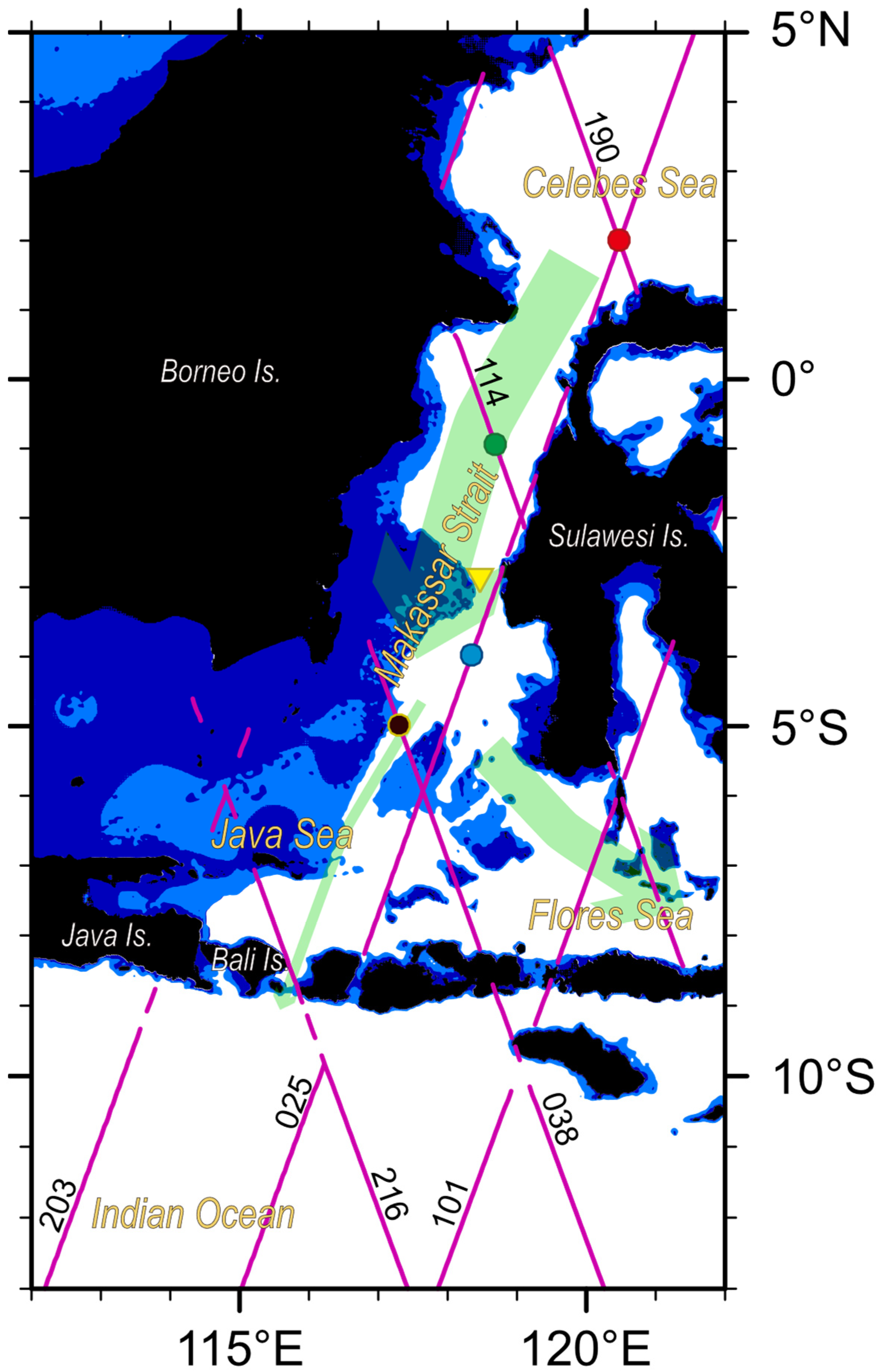
The Makassar Strait connects the Celebes Sea and the Java and Flores Seas (
Figure 1), and approximately 80% of the southward Indonesian throughflow (ITF) from the Pacific Ocean to the Indian Ocean is considered to pass this strait [
1]. Most areas of the southern part of the strait are shallower than 50 m, so deeper layers of the ITF are confined to the narrow (approximately 45 km width) Labani Channel. Long-term mooring with current meters in the Labani Channel has revealed that the currents in the Makassar Strait change in various time scales, but they have dominant seasonal variations, although semi-annual variations are also found in layers deeper than 300 m [
1].
Many researchers have investigated the ITF variations and related them to the sea level differences, or the pressure gradient force, at various time scales. Daily gridded satellite altimetry sea surface height (SSH) products are used in [
2] to obtain the SSH anomaly (SSHA) difference between the Celebes Sea and the Java Sea to discuss the Madden-Julian Oscillation (MJO). Term balances in the equation of motion in the along-strait direction reveal that both northward along-strait wind stress and northward pressure gradient over the Makassar Strait during the active phase of the MJO events will accelerate the northward ITF in the upper layers. Meanwhile, dominant seasonal variations in the upper-layer ITF have been found well correlated with both monsoon wind variations and the seasonal SSHA differences between the southwestern Pacific Ocean and the northeastern Indian Ocean that are also estimated from gridded satellite altimetry products [
3,
4]. Namely, the current in the Makassar Strait increases the northward component, or the southward ITF becomes weakened during the northwest Australian-Indonesian monsoon from December to March, and the SSHA in the northeastern Indian Ocean becomes higher than that in the southwestern Pacific Ocean. In addition, annual SSHA variations at three points in the central Makassar Strait, the southwestern Celebes Sea, and the northeastern Java Sea in another gridded altimetry product have been investigated to reveal that the seasonal SSHA gradient in the Makassar Strait is in phase with the SSHA difference between the Pacific and Indian Ocean [
5].
However, descriptions of these seasonal variations within the Makassar Strait are rather qualitative, and quantitative dynamic term balances, as investigated for the MJO in [
2], are not well discussed. In addition, the relationship between the pressure gradient force within the Makassar Strait and the external larger-scale SSHA difference between the Pacific and Indian Ocean is not understood well, although they are known in phase [
4]. For example, if the seasonal pressure gradient force variations between the Pacific and Indian Ocean directly produce the SSHA gradient in the Makassar Strait, uniform SSH gradient over the whole Celebes and Java Seas between the Pacific and Indian Ocean would be expected, but they have not investigated yet.
One reason the seasonal SSH variations within the Makassar Strait are not quantitatively discussed would be that standard satellite altimeter products are less reliable in a narrow strait than in open oceans [
6,
7]. Conventional satellite altimeters assume homogeneous reflection of microwave pulses at the sea surface, but this condition may not hold in areas close to coasts because of the occurrence of inhomogeneous microwave reflections by, e.g., lands, ships, and calm water in semi-closed ports [
8]. Therefore, in a narrow strait where most areas are close to coasts on both sides, the quality of altimetry observations is low. In addition, in the calm Indonesian Seas, small areas of smoother sea surface roughness (as known as “slicks”) that significantly reflect microwaves are often found even away from lands [
9,
10], so that the quality of standard altimeter datasets are further lower in this region.
In gridded SSH products, interpolations in time and space would relax those quality problems by filtering out outliers using the surrounding SSH data. In addition, spatial interpolation in gridded SSH products would also overcome problems with a less dense distribution of observation points [
11]. However, in coastal straits, SSH distribution within the strait could be strongly controlled by topography so that it could be significantly independent of SSH observations outside the strait. High-frequency ocean radar systems, which can provide dense observations of surface ocean currents in a limited coastal area, have revealed that currents in straits are so locally confined that simple spatial interpolations of sparse data coverage would not be able to account for this complexity [
6,
12]. In the Makassar Strait, which includes significant shallow bottom topography (
Figure 1), simple spatial interpolation in a gridded SSH product may erase characteristic SSH signals within the strait by referring uncorrelated data outside unless some sophisticated data assimilation techniques with complex physics accounts were used. This could be another reason dynamic term balances are not discussed quantitatively in the Makassar Strait.
Recently, however, new products have been developed to increase data availability in coastal areas [
13,
14]. The use of these coastal SSH products would enable us to discuss the dynamics of the seasonal SSH variations in the Makassar Strait quantitatively. The targets of this study are, therefore,
We use 17-year Jason coastal altimetry SSH products that can provide denser observation points with better quality, even in the narrow Makassar Strait.
We use those SSHA observations without spatial grid interpolations, although the data points become irregularly distributed.
Using quantitative SSHA gradient values, we investigate dynamic term balances of seasonal variations within the Makassar Strait.
By extending the study area outside the Makassar Strait (Celebes Sea, Java Sea, Flores Sea, and Pacific and Indian Ocean), we investigate the distribution of seasonal SSHA gradients around the Makassar Strait.
Then, we investigate the relationship between the seasonal SSHA gradient in the Makassar Strait and the seasonal SSHA difference between the Pacific and Indian Oceans.
We describe materials and methods in
Section 2, and then seasonal SSHA variations and dynamic balances within the Makassar Strait will be discussed in
Section 3. The seasonal SSHA variations around the Makassar Strait will be described in
Section 4 to investigate the relationship to the SSHA difference between the Pacific and the Indian Ocean. Factors that may affect the results will be discussed in
Section 5, and a summary and conclusions will be provided in
Section 6.
2. Materials and Methods
Since we dare to use non-gridded SSH data in this study, errors in a single SSH observation at a point may not be smoothed out using the surrounding SSH data. Therefore, the quality of single observations needs to be higher. In this study, therefore, we use the Adaptive Leading Edge Subwaveform (ALES) retracker Version 55 applied to Jason-series altimetry SSH data (Jason-1 from January 2002 to July 2008; Jason-2 from July 2008 to February 2016; Jason-3 from February 2016 to April 2019). Although the TOPEX/Poseidon satellite took the same tracks as the Jason series, no retracked data are available for the TOPEX/Poseidon mission. The ALES SSH data were produced by DGFI-TUM and distributed via OpenADB (
http://www.openadb.dgfi.tum.de, accessed on 15 January 2023). ALES dataset has been adjusted with fundamental range corrections used in standard products, like tropospheric, ionospheric, sea state bias, and dynamic atmosphere corrections. Tidal corrections (solid earth, load, ocean, and pole tides) are also applied; for ocean tides, the Empirical Ocean Tide (EOT) model produced by DGFI-TUM is used [
15]. More details on the retracker and the product are available in [
16,
17,
18].
We exclude all data that satisfy any of the conditions listed in
Table 1, as suggested by the data provider. In order to further reduce noises, the along-track 1-Hz SSH data are smoothed over five points (approximately 35 km long track) and nine cycles (approximately 90 days) with Gaussian weight function
, where
is the along-track distance,
is the temporal difference,
is the spatial smoothing scale (35 km), and
is the temporal smoothing scale (90 days); this process smooths out small-scale variations (thus called the Gaussian filter). Unlike the grid interpolation, which refers to far and sparse observations on different satellite tracks that may be located outside of bays or straits, the along-track smoothing can reduce the noises of each observation by referring to dense distributions (7 km separation) along the same track, and thus suitable for coastal studies [
6,
7,
9]. Note that the temporal smoothing also reduces residual errors in the corrections of aliased tides, except for the K
1 constituent whose aliased period is 173 days (e.g., [
19]).
The ALES SSH data refer to the mean sea surface data from the DTU15 model [
20], but in this study, we only use the SSHA data
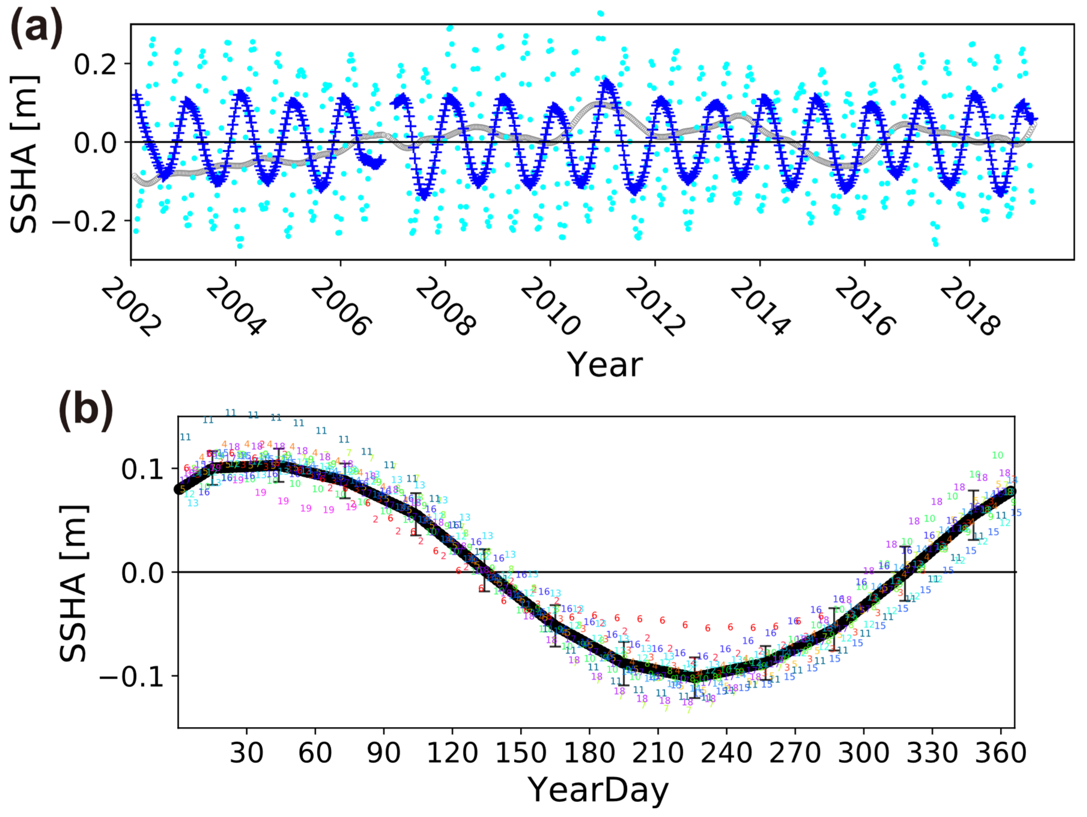
from the 17-year temporal mean. Near-annual SSHA variations
are then extracted from the time series of the SSHA data
at a point
by removing both variations longer than 13 months (
= 390 days) and shorter than 10 months (
= 300 days) using Gaussian filters (
Figure 2a). Namely, long-term variations
are first determined from
by the 13-month Gaussian filter. Then, the 10-month Gaussian filter applies to the residual component
to extract the near-annual SSHA variations
, and the residual component
becomes the short-term variations
.
In
Figure 2a, the largest magnitude of variations is found in the short-term variations.
. The root-mean-squared (RMS) values for
,
, and
in
Figure 2a are 0.15 m, 0.08 m, and 0.05 m, respectively. The short-term variations
obviously include nearly semi-annual variations, but as seen in
Figure 2a, the dates of peaks and troughs are not locked by annual year days but shifted during a long period. Indeed, the dominant period of
is approximately 173 days, so they would be dominated by aliased tidal errors of the K
1 constituent.
Meanwhile, as shown in
Figure 2b, all near-annual SSHA variations
show phase-locked similar seasonal changes, although they behave slightly differently each year. For example, maximum peaks are found in January or February, but the peak in 2011 around the year day 30 is significantly larger than those in the other years. Similarly, the minimum troughs are found in the boreal summer, but the trough in 2006 around the year day 240 deviates from those in the other years. These deviations could be related to the enhanced short-term variations
or long-term variations
, which could be caused by some interannual events such as El Nino/Southern Oscillation (ENSO) or Indian Ocean Dipole (IOD). However, they might be caused by unexpected data gaps in late 2006 (
Figure 2a). Therefore, we only focus on the 17-year mean seasonal variations in this study. The mean seasonal SSHA variations
are determined by taking the 17-year monthly mean from over 50 samples (three cycles in a month in a year). The data point will be discarded if the number of cycles used is less than a half of full observations.
To investigate dynamic balance with the pressure gradient force because of the SSHA gradient, we also use wind stress data and the ITF velocity data. The hourly velocity measurements from moorings maintained in the Labani Channel in the Makassar Strait from 1996 to 2017 are downloaded from
https://doi.org/10.7916/d8-p78a-zm51, accessed on 10 January 2023 [
21]. The data has been re-sampled at 20 m depth intervals between 40 and 760 m. The location of the mooring was marked using a yellow triangle in
Figure 1 at 2.8647°S, 118.4629°E. Following the past study [
1], the along-strait direction is defined as the axis rotated clockwise from the north by 10°. Note that no data was available for approximately two years, from July 2011 to August 2013.
Monthly averaged sea surface temperature (SST) and wind stress (
τ) values in the Makassar Strait (centered at 1°S, 118.5°E) are extracted from 0.25°-gridded “third-generation Japanese Ocean Flux Data Sets with Use of Remote Sensing Observations” (J-OFURO3) version 1.1 data [
22]. The duration of SST data is from 1988 to 2017, while that of the wind stress
τ is from 1991 to 2017. The along-strait component of the wind stress is extracted similarly to the ITF velocity.
We extract the mean seasonal variations from the time series of the ITF along-strait velocity, SST, and the along-strait wind stress, similar to the SSHA Gaussian filters. Although the durations of all datasets are different, we assume that all these durations are long enough to assume the mean seasonal variations of each dataset are not affected by either slight differences in durations or the presence or absence of interannual events such as ENSO and IOD.
3. Variations within the Makassar Strait
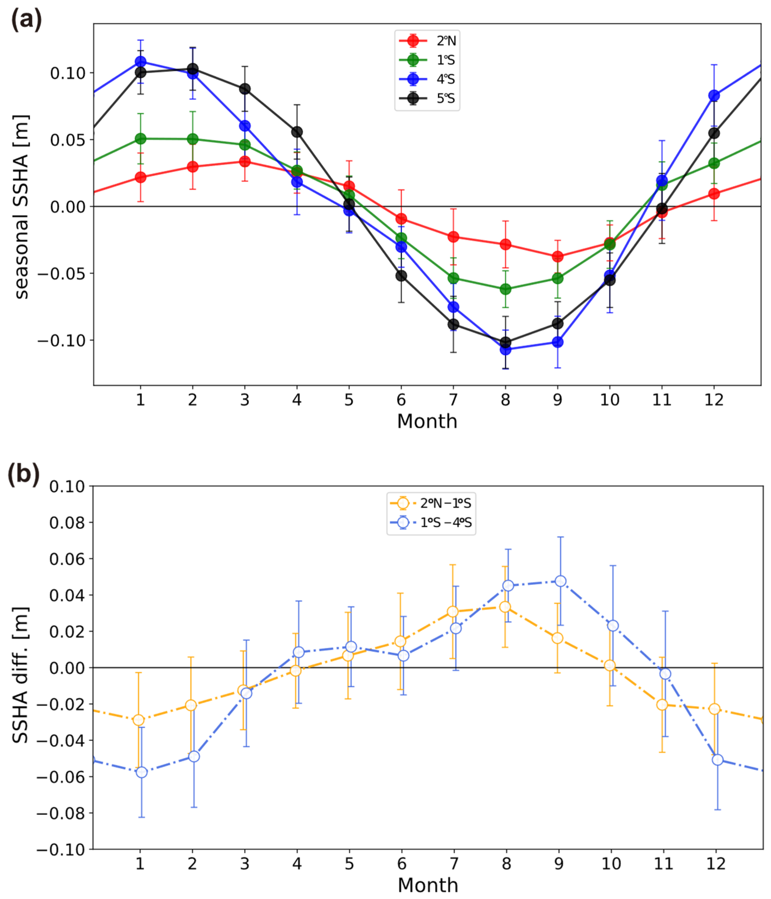
The non-gridded mean seasonal SSHA variations at four points in the Makassar Strait and the Celebes Sea (
Figure 1) are plotted in
Figure 3a. They are on different satellite tracks, so they are determined independently, but all variations are found in phase; positive values are found during the northwest Australian-Indonesian monsoon, December to March, while negative values are found during the southeast monsoon, June to September. Their half ranges from the minimums to the maximums, or amplitudes, are significantly larger than their standard deviations. The amplitude of these in-phase variations is monotonically increased from the northern points (2°N and 1°S) to the southern points (4°S and 5°S), as suggested in [
5].
However, as shown in
Figure 3b, the SSHA differences in the southern part of the Makassar Strait between 4°S and 1°S are significantly larger than ones in the northern part between 1°S and 2°N, whereas the spatial length of both pairs is approximately the same 400 km. This suggests that the SSHA gradient is not uniform in the Makassar Strait, and the larger SSHA gradients would be found to the north of 4°S or near the Labani Channel, where most areas of the strait are shallower than 50 m (
Figure 1).
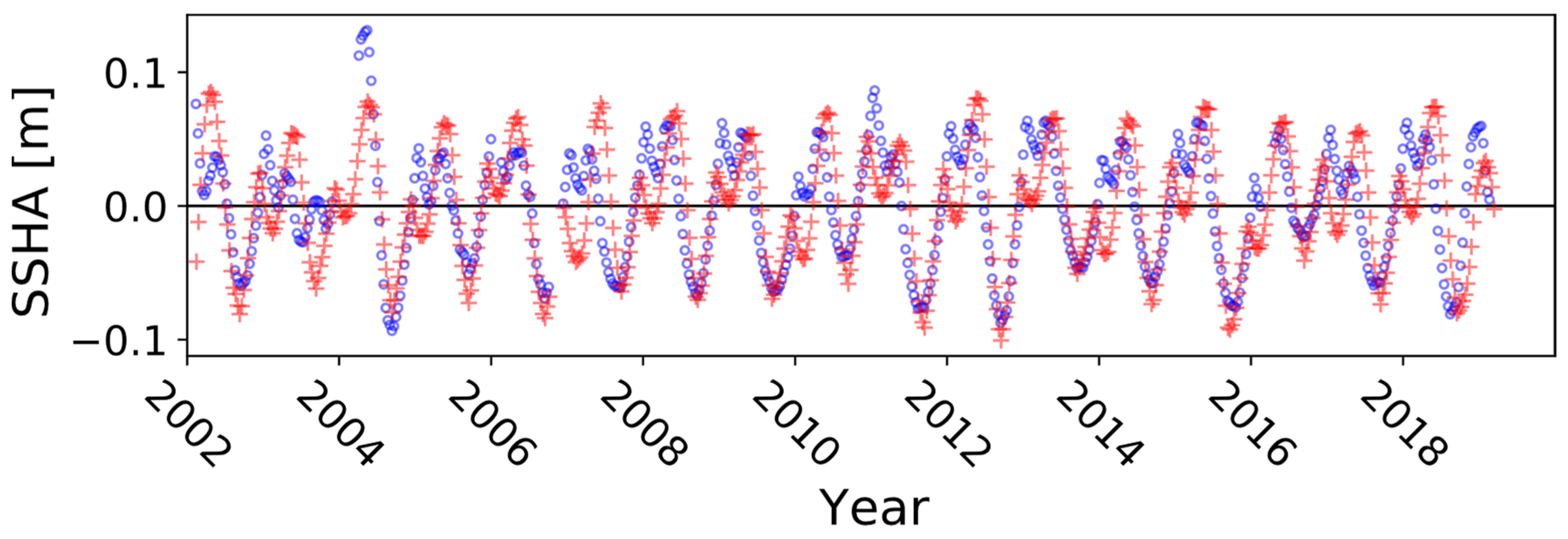
The mean seasonal SSHA variations in the southern part of the Makassar Strait at 5°S are compared to the other seasonal variations in
Figure 4. The SSHA variations (black bold line) agree well with the opposite phase of the along-strait wind stress component (blue broken line) with the significant Pearson correlation coefficient (CC) = −0.95. During the northwest (or southeast) monsoon from December to March (June to September), the along-strait wind component in the Makassar Strait is southward (northward). Similar phase variations with the SSHA (CC = 0.82) are also found in the along-strait ITF velocity component at the 40 m depth (yellow chain line), as the northward (or southward) anomaly is found during the northwest (southeast) monsoon, although the northward ITF anomaly ends slightly earlier in March than the end of the positive SSHA in May. Note that the seasonal SSH variations at 4°S (blue line in
Figure 3a), which is closer to the mooring site, show an earlier end of the positive SSHA in April and better CC = 0.92. All those similarities qualitatively agree with the past studies [
1,
3,
5].
Meanwhile, the ITF velocity at the 300 m depth (green chain line) shows significantly different variations. Semi-annual variations with peaks in November and May are significantly present [
1,
3,
23], suggesting that the ITF variations in the deeper layers are related to some other factors than the seasonal SSHA variations within the Makassar Strait.
Similarly, the seasonal SST anomaly variations (red dotted line) also show significant semi-annual variations with peaks in May and October. The discrepancy between the SST anomaly and SSHA would suggest that the seasonal SST anomaly variations would represent only a thin surface layer so that their steric height changes do not affect the SSHA. Indeed, the reported seasonal changes of the vertical temperature profile in the Makassar Strait in [
23] behave differently from these seasonal SST anomaly variations.
These seasonal variations are then quantitatively investigated in the dynamic equation of motion. Assuming the Coriolis force is negligible near the Equator, the equation of motion for the along-strait component in the upper layer can be written as the balance between the acceleration, the pressure gradient force, the wind stress, and the bottom friction terms: namely,
where
is the layer-averaged along-strait velocity component,
the along-strait SSHA gradient,
the acceleration of gravity,
the along-strait wind stress component,
the density of seawater,
the water depth, and
the linear bottom friction coefficient. Since the ITF velocity is not significantly strong, the equation can be linearized by removing the advection term, which allows us to discuss the seasonal component separately. Applying to the upper layer of the southern Makassar Strait near the Labani Channel, seasonal variations of these terms are calculated and plotted in
Figure 5, using
= 9.8 m s
−2,
= 1.03
10
3 kg m
−3,
= 50 m,
= 1.5
10
−4 m s
−1,
= the ITF velocity at the 40 m depth, and
= the SSHA gradient between 1°S and 4°S, the closest pair to the mooring site (
Figure 1). Note that the bottom friction coefficient
is not a determinant value, so we keep its typical order of magnitude as 10
−4 m s
−1 [
24] and inductively determined the fraction of
to obtain reasonable variation ranges is in
Figure 5.
Both wind stress and bottom friction terms have reversed phases with the pressure gradient term so that both can be qualitatively balanced with the pressure gradient term (
Figure 4 and
Figure 5). However, the magnitude of the wind stress term in
Figure 5 is significantly smaller than that of the other terms. Since the SSHA gradients are not uniform within the Makassar Strait, as suggested in
Figure 3b, the pressure gradient term could be smaller than one plotted in
Figure 5 if we include areas other than the Labani Channel. Still, however, the pressure gradient term is too large with respect to the weak wind stress over the Makassar Strait. Note that the dynamic term balances investigated for the MJO in [
2] are of the order of 10
−8 m s
−2, which are close to that of the wind stress term shown in
Figure 5. In other words, the seasonal SSHA gradient in the Makassar Strait, seen in
Figure 3, is significantly larger than the SSHA gradient seen in the MJO, and only the bottom friction term would balance this large seasonal pressure gradient term. Note that both wind stress and bottom friction terms include the depth
so that their magnitude ratio does not depend on
. The selection of
would affect the balance between the bottom friction term and the pressure gradient term, but it also depends on the non-determinant parameter
.
Note that the acceleration term in
Figure 5 is not only too small but also its phase is shifted from that of the other terms, as its maximum value appears in November, in which the other terms become almost zero. This would suggest that the ITF velocity is not directly accelerated by a single term in Equation (1).
4. Variations around the Makassar Strait
In the previous section, we have seen that the seasonal SSHA variations are in phase over the whole Makassar Strait, with their amplitude strengthened in the southern part, as suggested by [
5]. To examine this tendency outside the Makassar Strait, we have applied the same processes (i.e., nine cycle and five points smoothing 10-month and 13-month Gaussian filters and monthly averaging over 17 years) to obtain the mean seasonal SSHA variations at additional 50 points in and around the Makassar Strait (the Celebes Sea, the Java Sea, the Flores Sea, the southwestern Pacific Ocean, and the northeastern Indian Ocean) together with four points in
Figure 3a. Then, CC with the seasonal SSHA variation at the point 5°S, 117.3°E (shown in
Figure 2b) is calculated for each point (
Table 2).
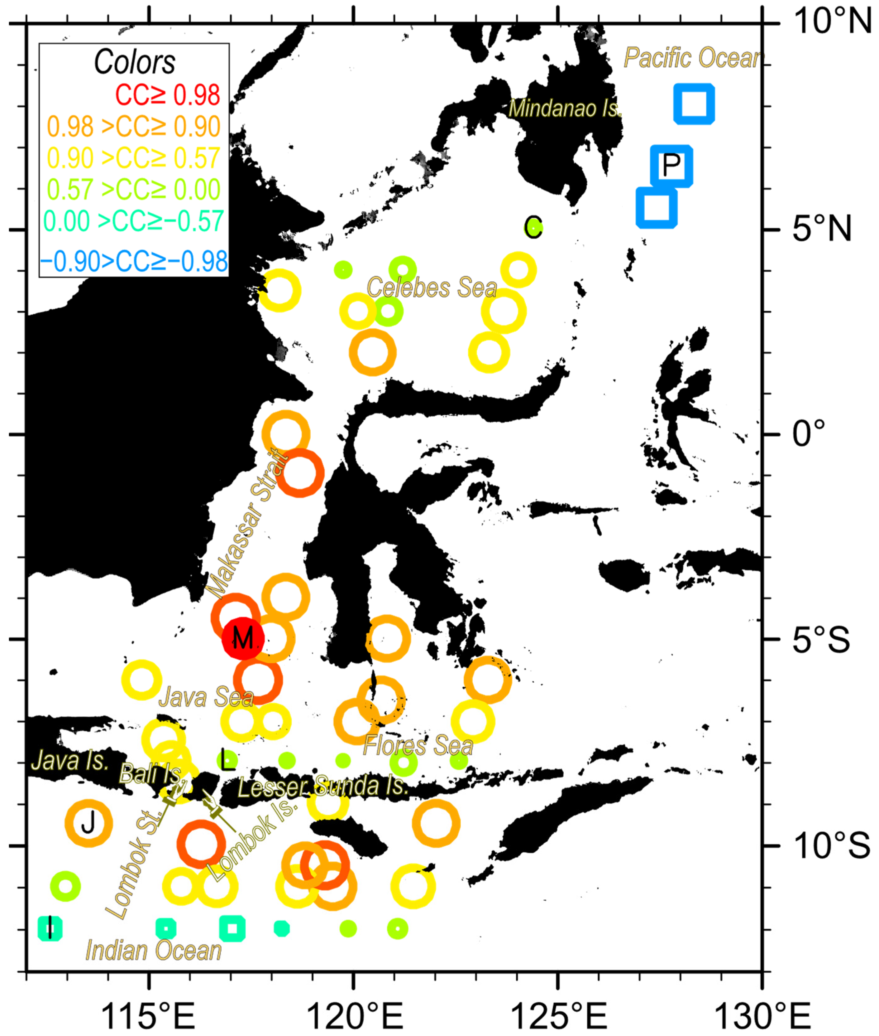
Figure 6 shows the spatial distributions of CC. The CC is colored with criteria values 0.98, 0.90, and 0.57, which are selected so that the CC differences (0.98 and 0.90, or 0.90 and 0.57) become significant with a 99% confidence level using Fisher’s Z-test with 12 monthly samples.
All data points within the Makassar Strait, including three points not included in
Figure 3a, are in phase so that their correlation coefficient is larger than 0.97 (red and orange circles in
Figure 6). In the Celebes Sea, however, the distribution of CC is different in the northern and southern parts. The largest CC = 0.94 is found at 2°N, 120.5°E (Point Number 10), the closest point to the northern Makassar Strait (red circle in
Figure 1), then moderate CC values larger than 0.57 (yellow circles) are present in the southern Celebes Sea. However, in the northern Celebes Sea where is away from the Makassar Strait, CC decreases as lower than 0.54 (green circles). For example, the point in the northeastern Celebes Sea at 5°N, 124.4°E (Point Number 4; marked as “C” in
Figure 6) has small CC = 0.26 (
Table 2). Similarly, in the northern Java Sea, CC becomes smaller as the distance from the Makassar Strait increased.
In the Flores Sea, contrasts between the northern and southern parts become clearer. In the northern part, CC values are larger than 0.9, as shown by orange circles in
Figure 6, even at points far from the Makassar Strait. However, CC values along the northern coast of the Lesser Sunda Islands in the southern part of the Flores Sea are significantly low, as shown using small green circles. The low CC value along the northern coast is also seen in the southern Java Sea, as CC is only 0.30 at the point northeast of Lombok Island, 7.9°S, 116.9°E (Point Number 24; marked as “L”).
On the contrary, high CC values are found along the southern coast of the Java and Lesser Sunda Islands. Those high CC values are, however, confined only near the coasts so that offshore points in the Indian Ocean show small or weakly negative correlations. The point south of Java Island at 9.5°S, 113.5°E (Point Number 38; marked as “J”) has a significantly high CC = 0.96, but its 300 km offshore point at 12°S, 112.6°E (Point Number 49; marked as “I”) has a negative CC = −0.41.
More significant negative correlations are found in the southwestern Pacific Ocean. The CC = −0.96 is found at the point 6.5°N, 127.8°E (Point Number 2), marked as “P” in
Figure 6. Surrounding points similarly have significant negative correlations, as shown using light blue and cyan squares, in contrast to small positive CC values at the adjacent points in the northeastern Celebes Sea.
For more insight, the seasonal SSHA variations in the above six marked points are plotted in
Figure 7. Clear in-phase relationships with the monsoon are found in the Makassar Strait (M; black line), along the southern coast of Java Island (J; red line), and oppositely in-phase in the southwestern Pacific Ocean (P; blue line). At other locations in the northern Celebes Sea (C; cyan chain line) and in the offshore Indian Ocean (I; orange broken line), their phases do not correspond to the monsoon seasons. Especially, the SSHA variations at the point northeast of Lombok Island (L; purple dotted line) have double peaks in May and December, which differ significantly from the SSHA variations in the Makassar Strait and are rather similar to the seasonal variations of the deep-layer ITF velocity shown in
Figure 4.
The SSHA difference between point “P” in the southwestern Pacific Ocean and point “J” south of Java Island would reach nearly 0.2 m, which is larger than the SSHA difference within the Makassar Strait shown in
Figure 3b so that this SSHA difference will become a good index that is in-phase with the seasonal SSHA variations in the Makassar Strait. However, adjacent seasonal SSHA variations in the northern Celebes and southern Java Seas disconnect those SSHA variations in the Pacific and Indian Ocean, and therefore, the SSH difference between “P” and “J” points would not directly drive the SSHA gradient within Makassar Strait.
In
Figure 7, the amplitude of the seasonal SSHA variations at the point “J” south of Java is slightly larger than that in the southern Makassar Strait “M”, although the range discrepancy does not substantially exceed the standard deviations at the point “J”. As seen in
Figure 7, the standard deviation at point “J” is significantly larger than that at point “M”, suggesting that the near-annual SSHA variations
south of Java Island include large interannual variations than ones in the Makassar Strait, shown in
Figure 2b.
To investigate spatial distributions of the amplitude of the seasonal SSHA variations that are in phase with the SSHA in the Makassar Strait, the least square fitting method is introduced. Namely, the seasonal SSHA variations at a given point,
, would be written as
where
is the seasonal SSHA variations at the point “M” (5°S, 117.3°E) in the Makassar Strait (Point Number 18 in
Table 2),
is the amplitude factor of the fitted variations, and
is the independent residual SSHA variations that are not in phase with
. The unknown
A is determined to minimize the sum of squared difference
. Namely,
The fitting would be meaningful only when the independent variations
are negligibly small with respect to the fitted variations
. Therefore, we introduce the dominance ratio
d as the ratio of the variance of the fitted variations
(t) to the variance of the original SSHA variations
; namely,
In other words,
A would not be meaningful if
d were not large enough. The amplitude factor
A and the dominance ratio
d are calculated for all 54 points (
Table 3).
By substituting Equation (3) to (4),
d can be transformed as:
As expected from Equation (5), the characteristics of
d are close to those of CC in
Table 2. Namely, both
d and the magnitude of CC are high within the Makassar Strait, along the southern coast of the Java and Lesser Sunda Islands, in the northern Java and Flores Seas, and in the southwestern Pacific Ocean. On the contrary, they are significantly small along the northern coast of the Lesser Sunda Islands (in the southern Java and Flores Seas). Hereinafter, we will mainly use points whose
d exceeds 0.8 or CC exceeds 0.89 to investigate the spatial distribution of
A. Points with
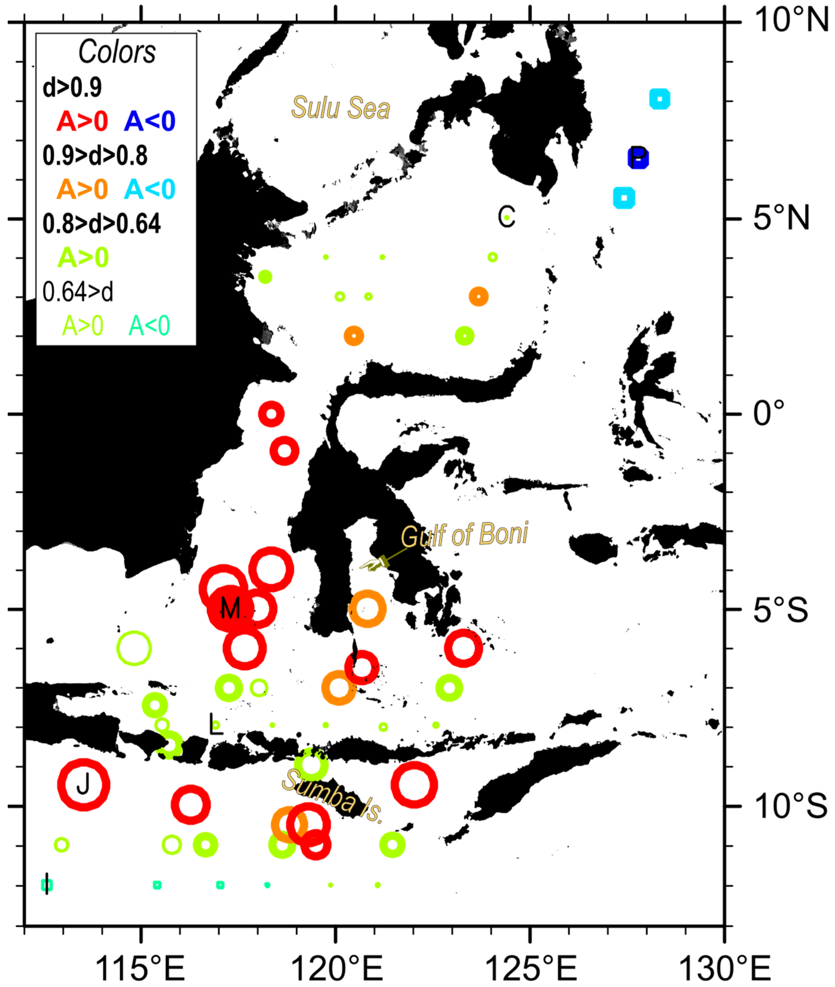
d exceeding 0.64 or CC exceeding 0.80 are supplementary used.
The distribution of
A is mapped in
Figure 8 as the sizes of markers. In the Makassar Strait and adjacent northern Java and southern Celebes Seas, the northward decreasing tendency is confirmed, as explained in
Figure 3a. More precisely, the maximum
A = 1.05 is found at 4.5°S, 117.1°E (Point Number 17 in
Table 3), near the edge of 50 m isobath (
Figure 1). As the distance from this point increases, the amplitude
A becomes smaller. This tendency is still found in the northern part of the Makassar Strait (north of 3°S) as
A = 0.55 to 0.46, and even in the southern Celebes Sea as
A = 0.31 to 0.30, although the decreasing ratio of
A is significantly smaller than that in the southern part of the Makassar Strait. This confirms that the largest horizontal SSHA gradient by this in-phase seasonal variation would occur in the Makassar Strait between 4°S and 1°S over the narrow Labani Channel.
On the other hand, in the northern part of Flores Sea east of 120°E and north of 7°S, the maximum
A = 0.78 is found at the eastern point 6°S, 123.3°E (Point Number 36), while the second largest
A = 0.76 is at 5°S, 120.8°E (Point Number 32), in the Gulf of Boni south of Sulawesi Island. These distributions in the northern Flores Sea do not follow the distance-determined relationship seen in the Makassar Strait, and it rather suggests that the distance from coasts of large islands determines the magnitude of
A. Similarly, in the Indian Ocean, points with larger
d are confined to coastal areas south of Java and the Lesser Sunda Islands. Extra-large
A = 1.14 is found at 9.5°S, 113.5°E (Point Number 38), south of Java Island, marked using “J” in
Figure 8, but no significant
components are found at the offshore point (11°S, 113°E; Point Number 43) that is 170 km away from point “J”. Around 119°E and along the southern coast of Sumba Island, maximum
A = 0.93 occurs at a point 10.5°S, 119.3°E (Point Number 42) closest to the island, then
A decreases to 0.73 (10.5°S, 118.8°E; Point Number 41) and 0.58 (11°S, 119.5°E; Point Number 47), and
A becomes 0.50 at the offshore point 11°S, 118.6°E (Point Number 46).
Together with their in-phase relationship with the monsoon seasons, the coastally confined characteristics in
Figure 8 in the Indian Ocean and in the northern Flores Sea would suggest that these SSHA variations are caused by the divergence or convergence of surface wind-driven transport by coastal walls of large islands. Namely, during the northwest (or southeast) monsoon period from December to March (June to September), the eastward (westward) wind component is found over these areas, producing an increase (decrease) of SSH along the southern coast of large islands.
Similarly, within the Makassar Strait, although the maximum amplitude
A is found away from the coastal wall boundaries of large islands, wind-driven currents over shallow areas can also generate SSHA gradients, especially when the depth is as shallow as the surface boundary layer thickness [
25]. This would explain why the largest SSHA variations in the Makassar Strait occur at the southern shallow point.
In the Pacific Ocean, all three points have significant d and similar negative A values. These points are also far from the coastal walls of large islands, but variations in wind speeds and the Coriolis parameter can produce the convergence or divergence of wind-driven transport. Namely, during the northwest (or southeast) monsoon period from December to March (June to September), both enhanced Coriolis parameter and higher southwestward (northeastward) wind speeds at higher latitudes would produce divergence (convergence) of wind-driven transport at those points, resulting in lower (higher) SSHA variations.
5. Discussion
If the convergence or divergence of wind-driven transport by coastal walls is the dominant factor along the southern coast of the Lesser Sunda Islands, the reversed in-phase relationship could be symmetrically expected on the northern coast, accounting for large spatial scales of wind directions. Namely, negative
A values with large
d could be present along the northern coast of the Lesser Sunda Islands in
Figure 8, as seen at points in the Pacific Ocean. However, their
d values are found to be significantly small (
Table 3). We recall that the actual seasonal SSHA variations at the point “L” (7.9°S, 116.9°E; Point Number 24) have intra-seasonal variations with double peaks in May and December (
Figure 7), which are significantly different from the monsoon seasons. This suggests that other significant factors than the convergence of local wind-driven transports should be present in the southern part of the Java and Flores Seas.
The same least square fit in Equation (2) but using the seasonal SSHA variations at the point “L” (Point Number 24) instead of
is plotted in
Figure 9 and is listed in
Table 4. Only three points have significant
d values, all of which are along the northern coast of the Lesser Sunda Islands and only to the east of point “L” (
Figure 9). To the northwest of the Lombok Strait, no points have significant dominance ratio
d, except a point to the north of Bali Island (7.9°S, 115.5°E; Point Number 22) with moderate
d = 0.69 (or CC = 0.83). This suggests the existence of different signals to the west and east of the Lombok Strait. Past studies on intra-seasonal variations in the Indonesian Seas (e.g., [
26,
27,
28]) suggest different propagation routes of the Kelvin waves in the Java and Flores Seas. Some of the Kelvin waves propagating eastward along the southern coast of Java and Bali islands enter the Java Sea through the Lombok Strait and propagate westward along the northern coast of Bali Island and then northeastward toward Kangean Island along shallow isobaths (
Figure 1 and
Figure 9). The other part of the Kelvin waves continue propagating along the southern coast of the Lesser Sunda Islands and enter the Flores Sea through the Ombai Strait, and they propagate westward along the northern coast [
28]. At the point “L”, therefore, the Kelvin waves would take the latter route along the northern coast of the Lesser Sunda Islands, only to the east of the Lombok Strait. Note that in the offshore Indian Ocean in
Figure 9, a long train of points with moderate
d is found along 11°S or 12°S, even to the east of the Lombok Strait.
In this study, only near-annual variations are focused, partly because the aliased K
1 constituent (173 days period) could contaminate altimetry-derived SSHA variations. However, intra-seasonal components are found in
Figure 7 at the point “L”. The Gaussian filter works well to remove sinusoidal variations, such as aliased tidal constituents, but is less effective for signals with a larger kurtosis, such as intermittent pulses. Therefore, although variations shorter than 10 months are mostly filtered out in this study, significantly large intermittent pulses would not be fully removed using the Gaussian filter so that they could remain in the near-annual data. In order to confirm this, the near-annual variations
at the point “L” are plotted in
Figure 10. They include pulse-like short-term SSHA changes, which are not observed in
Figure 2a in the Makassar Strait. The RMS values for short-term variations
, near-annual variation
, and long-term variations
at the point “L” are 0.17 m, 0.04 m, and 0.03 m, respectively, which confirms that the short-term variations are significantly large at the point “L”. It should be also noted that most of these pulses in
Figure 10 are phase-locked in the annual year days. We recall that the aliased K
1 constituent are not phase-locked in the annual year days as seen as
in
Figure 2a, so that the aliased K
1 tidal errors would be removed in the mean seasonal SSHA variations
.
The near-annual SSHA variations
at another point south of Kangean Island (7.4°S, 115.4°E; Point Number 21) are also plotted in
Figure 10 for reference. This point is along the suggested pathway of the Kelvin waves from the Lombok Strait (
Figure 9). Since the dominance ratio
d = 0.49 (CC = 0.7) is small at this point, the SSHA variations should include some independent variations that are not in phase with the SSHA variations at point “L”. The near-annual SSHA variations
at Point Number 21 also include pulses but with different phases from the ones at point “L”. These results are consistent with the concept of different pathways of the Kelvin waves.
Note that semi-annual components are also found in the ITF velocity at the 300 m depth (
Figure 4), which are suggested to be related to the intra-seasonal Kelvin wave propagations in the southern part of the Java Sea [
23]. However, we do not quantitively focus on these intra-seasonal variations and leave them for future studies since the intra-seasonal variations would be significantly underestimated in this study by applying the Gaussian filters.
Some researchers suggest the potential contribution of injection of distinct water mass from the South China Sea into the southern Makassar Strait through the Java Sea (South China Sea throughflow, e.g., [
29,
30,
31]), but this contribution cannot be discussed in this study since the injection paths are over the shallow areas where no SSHA data points are available. However, in
Figure 8, significant
d values for the mean seasonal SSHA variations
in the southern Makassar Strait are found even in the southern Celebes Sea, which cannot be explained using the South China Sea throughflow alone. Instead, note that points in the northern Celebes Sea have significantly smaller
d values, which could be affected by inflow from the Sulu Sea.
6. Summary and Conclusions
Using along-track Jason-series data from 2002 to 2019 processed with the ALES retracker that can produce better-quality SSH observations in coastal areas, the mean seasonal SSH variations in and around the Makassar Strait are investigated. All data points are processed without spatial grid interpolation so that they can independently observe small-scale features around narrow straits and bays without producing pseudo signals by over-smoothing from far data points, although data point distributions become irregular.
The seasonal SSHA variations are confirmed in phase with the monsoon seasons at all points from the southern Celebes Sea to the northern Java Sea through the Makassar Strait. By applying the least square fitting of the seasonal SSHA variations at a point in the Makassar Strait, the largest amplitude of the in-phase variations is found at a point near the southern end of the Makassar Strait and near the 50 m isobath. As the distance from this point increases, the amplitude becomes smaller, producing horizontal SSHA gradients, i.e., the pressure gradient forces. The SSHA gradients are not uniform over the area, and the largest gradient is found between 4°S and 1°S in the Makassar Strait, over the narrow Labani Channel.
Since the pressure gradient force in the Makassar Strait is reversely in phase with the along-strait wind stress and the bottom friction of the surface ITF velocity, both can qualitatively balance with the pressure gradient force. Quantitatively, however, the wind stress is found too weak (approximately 0.5 10−8 m s−2) to balance the pressure gradient force (approximately 1.5 10−6 m s−2), suggesting that the pressure gradient force in the Makassar Strait is balanced with the bottom friction of the surface ITF velocity over the shallow-depth area, which is a significant topographic characteristic of this strait.
Similar in-phase seasonal SSHA variations are also found along the southern coast of Java and Lesser Sunda Islands, in the northern Flores Sea, and reversely in-phase in the southwestern Pacific Ocean. The areas in the Pacific and Indian Ocean are, however, isolated from the Makassar Strait by adjacent areas with uncorrelated SSHA variations, and thus, they do not directly force the SSHA gradient within the Makassar Strait. All of those in-phase seasonal SSHA variations would be caused by the convergence or divergence of local wind-driven transports.
Along the northern coast of the Lesser Sunda Islands, significant intra-seasonal SSHA variations are found, which could be related to the semi-annual ITF variations in the lower layer. However, since this study focuses on the mean seasonal variations, both intra-seasonal variations and interannual variations with ENSO and IOD events would be left for future studies.
These results can be summarized in short:
Seasonal monsoon wind variations produce seasonal SSHA changes along coastal walls of large islands or over shallow areas.
All those SSHA variations are in phase, even though they are generated independently.
Large in-phase SSHA variations occur south of Java Island, while reversed in-phase variations are generated in the southwestern Pacific Ocean. Therefore, we can obtain a clear in-phase index by taking the difference between those SSHA variations.
Along the northern coast of the Lesser Sunda Islands and in the northern Celebes Sea, the seasonal SSHA variations are out of phase from the monsoon seasons. Therefore, the SSHA variations in the Pacific and Indian Ocean are dynamically isolated from the seasonal SSHA variations within the Makassar Strait using uncorrelated SSHA variations in the adjacent areas.
In an area from the northern Java Sea to the southern Celebes Sea through the Makassar Strait, the seasonal SSHA variations are in phase, but their amplitude decreases toward the north, producing horizontal SSHA gradients. The largest SSHA gradient is found between 4°S and 1°S in the Makassar Strait, over the narrow Labani Channel.
The pressure gradient force caused by the SSHA gradient is balanced with the bottom friction of the surface ITF velocity in the Makassar Strait since the wind stress over the strait is too weak.


