Author Contributions
Conceptualization, C.T., M.M.M. and S.D.; methodology, M.M.M., C.T., S.D. and M.N.; software, M.N., M.M.M. and S.D.; validation, M.M.M., M.N., F.B. and J.Z.; formal analysis, M.M.M., M.N., S.D. and J.L.; investigation, M.N., M.M.M., S.D, F.B. and J.Z.; resources, M.M.M., S.D, M.N., C.T. and M.N.; data curation, M.N., M.M.M. and S.D.; writing—original draft preparation, M.M.M., M.N. and S.D; writing—review and editing, M.M.M., S.D., M.N., C.T., J.L., C.D., J.Z. and S.H.; visualization, M.M.M. and M.N.; supervision, C.T., S.H. and C.D.; project administration, C.T. and S.H.; funding acquisition, C.T. All authors have read and agreed to the published version of the manuscript.
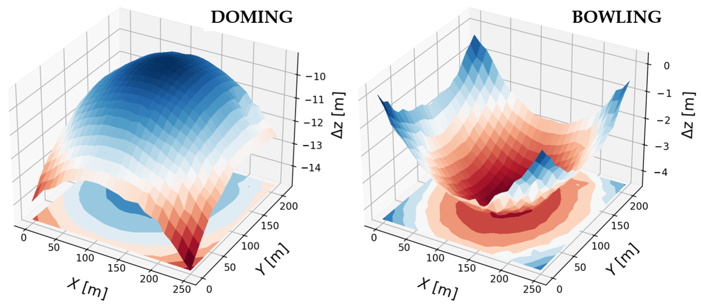
Figure 1.
Examples of 3D model systematic deformations (bowling and doming) investigated in this study.
Figure 1.
Examples of 3D model systematic deformations (bowling and doming) investigated in this study.
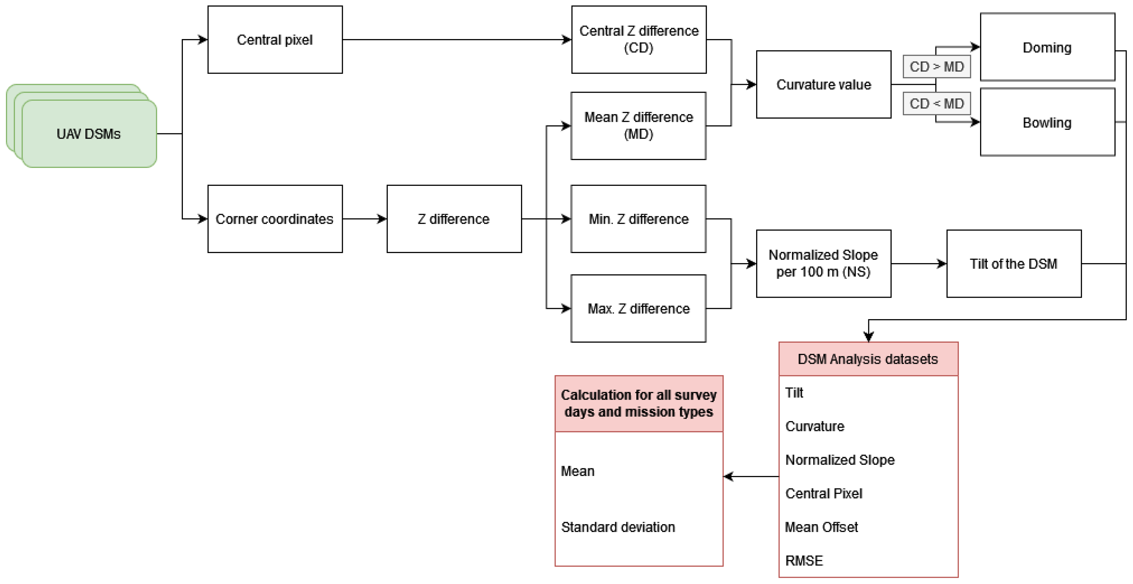
Figure 2.
Workflow of processing the SfM-MVS based HDMs. Green/yellow = input data, white = processing, red = output data. HDM = height difference model.
Figure 2.
Workflow of processing the SfM-MVS based HDMs. Green/yellow = input data, white = processing, red = output data. HDM = height difference model.
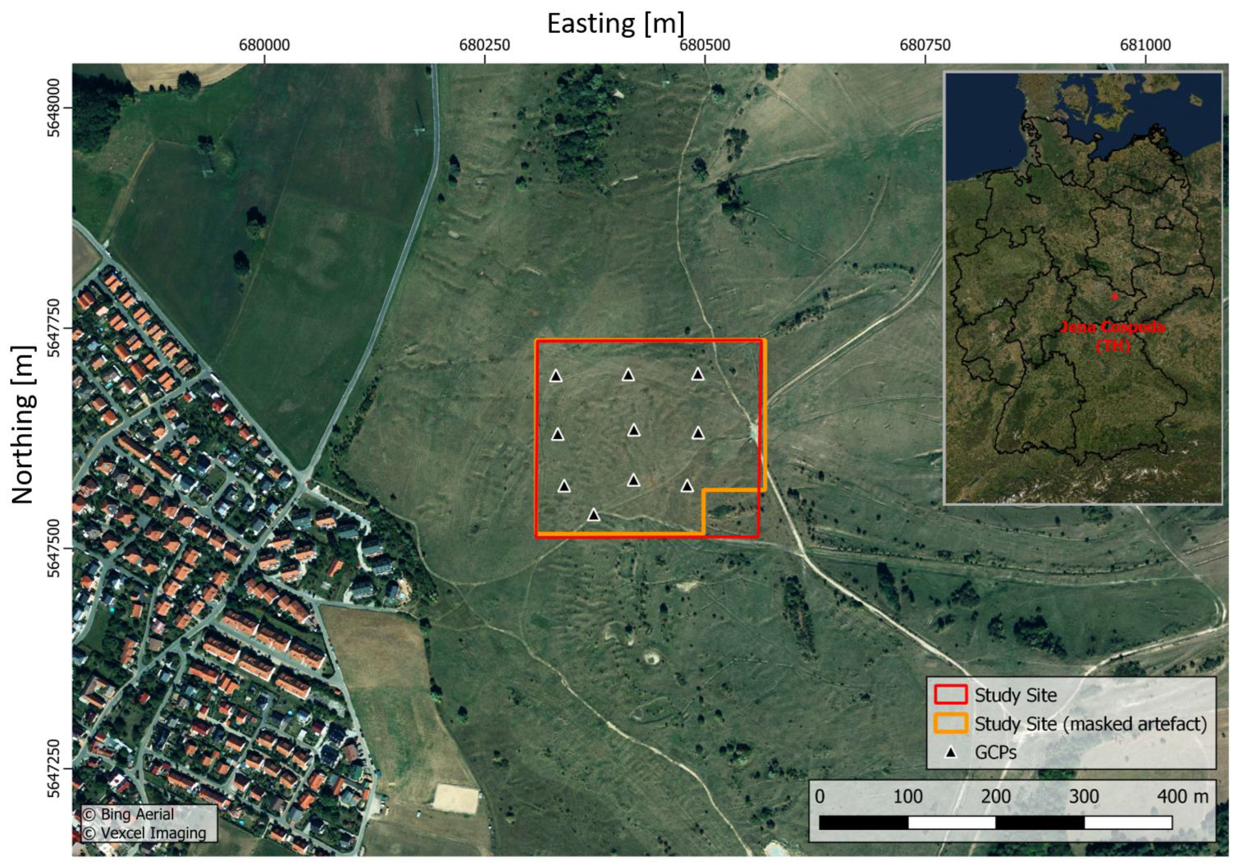
Figure 3.
Map of the study area (red) and masked study area (orange) with the locations of ten ground control points (black), all datasets are projected in WGS 84/UTM zone 32N. The Jena district of Cospeda is located in the western area. The city of Jena is located to the south of the study area.
Figure 3.
Map of the study area (red) and masked study area (orange) with the locations of ten ground control points (black), all datasets are projected in WGS 84/UTM zone 32N. The Jena district of Cospeda is located in the western area. The city of Jena is located to the south of the study area.
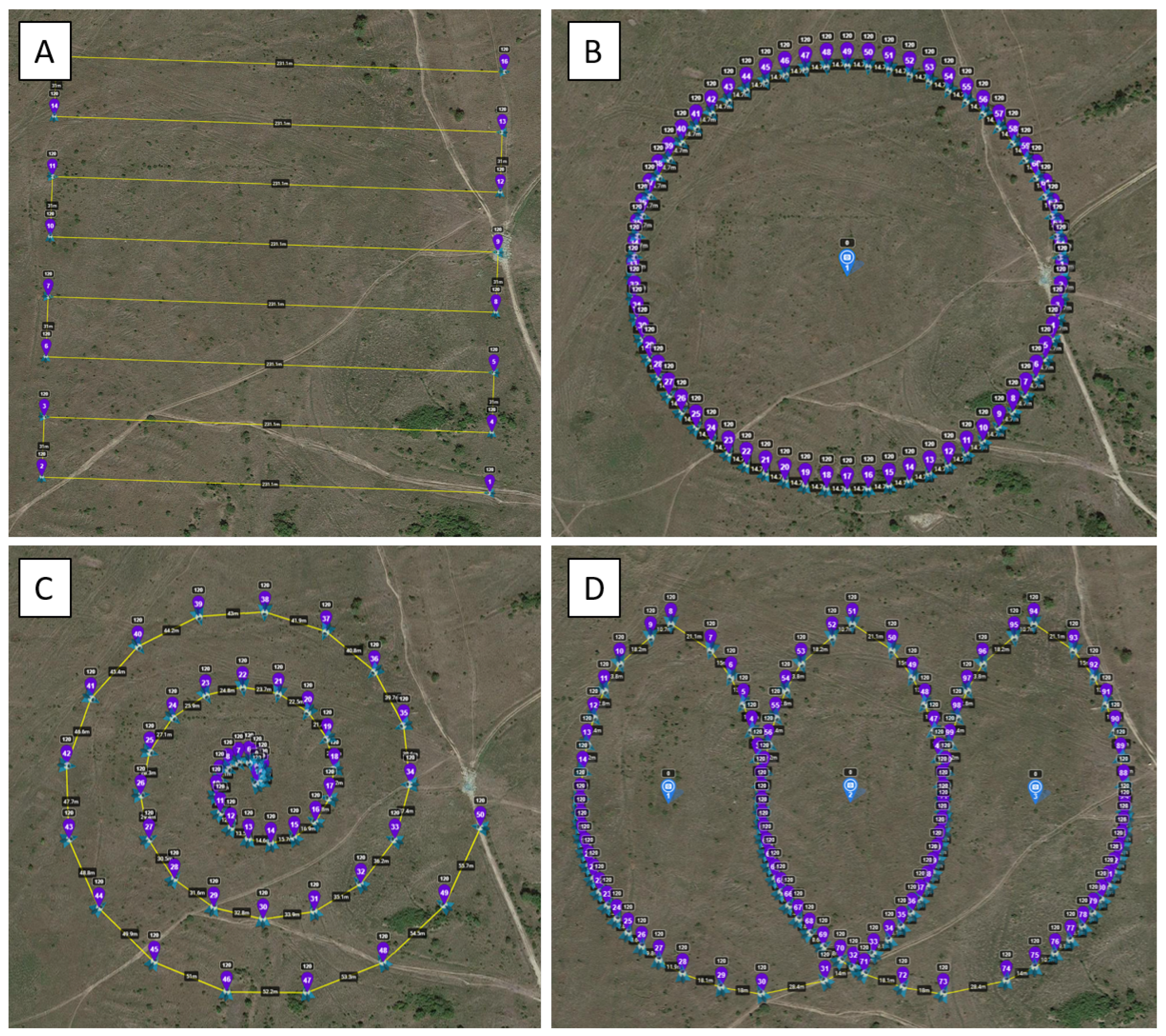
Figure 4.
(A) Nadir and oblique view flight plan, the markers (purple) show individual waypoints on the UAV’s flight paths (yellow). The camera captures the image data with an angle of 0° (nadir flight pattern) and off-nadir angle of 30° (oblique view images). (B) POI flight plan, where the UAV circles the reference point (camera symbol in the center of the circular flight path) on the flight path. (C) Spiral flight plan where the UAV orbits the center reference point on the flight path in a spiral orbit. (D) Loop flight plan with three reference points (camera symbols), around which the UAV circles in an elliptical pattern. All figures are taken from the “Mission Hub” of the “Litchi” application.
Figure 5.
The extraction of curvature and slope deformation was performed by focusing on the central and edge pixels, leading to the computation of digital surface model (DSM) analysis products. These products were then employed to interpret the effects of deformation associated with various flight designs.
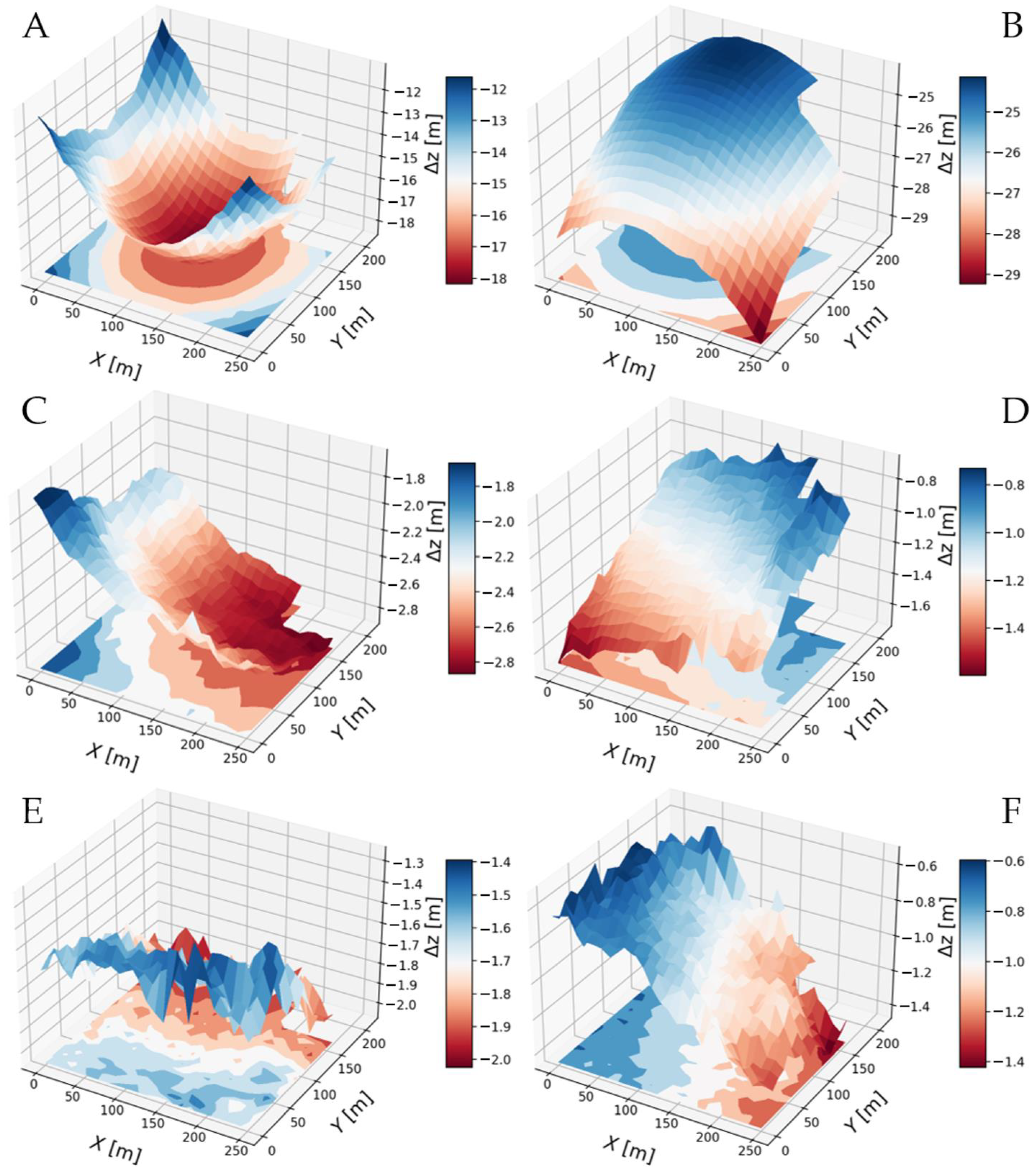
Figure 6.
3D visualization of the different distortion effects observed in this study. Doming effect of the Nadir_120m flight mission on 19 May 2022 (A), bowling effect of the Nadir_120m flight mission on 10 May 2022 (B), slight doming effect of the Oblique_120m flight mission on 5 July 2022 (C). The other flight designs (POI_120m on 10 May 2022 (D), Spiral_120m on 10 May 2022 (E), Loop_120m on 18 May 2022 (F)) all show a varying degree of tilted distortions with no dominant tilt direction. It should be noted that the Δz-axis (z-offset) range is different for each subplot.
Figure 7.
Distribution of the angle intersections of the epipolar lines of all tie points for each mission design at 120 m flight altitude (POI: red, nadir: green, loops: blue, spirals: black, oblique: orange) and total number of intersections per mission design.
Figure 7.
Distribution of the angle intersections of the epipolar lines of all tie points for each mission design at 120 m flight altitude (POI: red, nadir: green, loops: blue, spirals: black, oblique: orange) and total number of intersections per mission design.
Table 1.
Overview of relevant scientific publications on the additional and exclusive use of oblique images to increase Z-accuracy. Additionally, different camera angles, heights, and image overlaps are examined.
Table 1.
Overview of relevant scientific publications on the additional and exclusive use of oblique images to increase Z-accuracy. Additionally, different camera angles, heights, and image overlaps are examined.
| Ref. | Hardware | Gimbal | Altitude | Site | Area | Overlap (%) | Oblique Effect |
|---|
| [4] | DJI Phantom 4 Pro (3×) | Nadir, oblique, POI | 35–65 m | Urban, flat | 2.1 ha | 65/45 | Doming sizes: nadir: 0.813 m, oblique: 0.149 m, POI: 0.101 m, nadir + ob: 0.082 m |
| [19] | Canon 550D | Nadir, POI | 20–25 m (nadir), 18 m (POI) | Nature, River | 3.5 ha | 80/90 | Significant improvement in horizontal and vertical accuracy |
| [22] | DJI M210, senseFly eBee X, DJI Mavic Pro | Nadir, oblique | 80–100 m | Permafrost | 0.3–0.5 ha | 70/80 | Increases z-accuracy significantly (MAE from 0.2 m (nadir) to 0.03 m (nadir + oblique)) |
| [24] | DJI Phantom 4 RTK | Nadir, oblique | 30–60 m | Hilly, steep ravines | n.a. | n.a. | Nadir significantly higher standard deviation and mean error than oblique images or combination of nadir and oblique images |
| [37] | Canon 450D | Nadir, oblique | Varying | Volcanic rock sample | n.a. | n.a. | Reduce the doming effect by up to two orders of magnitude |
| [45] | DJI Phantom 3 Pro | Nadir, oblique, POI | 49 m | Flat, hilly | 27.4 ha | 80/70 | Improved accuracy by 5 to 9 orders of magnitude |
| [46] | FlyNovex | Nadir, oblique | 90 m (nadir), 50 m (oblique) | Urban | n.a. | 80/75 (nadir), 80/80 (oblique) | 50–90% improvement in accuracy |
| [47] | DJI Phantom 3 Pro | Nadir, oblique | 40 m | Hilly | 0.7 ha | 90/90, 90/70, 70/70 | Accuracies of oblique images in the range 20–35° higher than oblique images 0–15° |
| [48] | DJI Phantom 4 Pro | Nadir, oblique | 65 m | Plateau, steep ravines | n.a. | 80/80 | Error reduction up to 50% |
| [49] | DJI Phantom 4 RTK | Nadir, oblique | 100 m (nadir), 75/125 m (oblique) | Fallow land, rural | n.a. | 75/75 | Combination nadir + oblique with best results, higher oblique angles with better results |
Table 2.
UAV specifications of DJI Mini 2 [
58].
Table 2.
UAV specifications of DJI Mini 2 [
58].
| UAV | DJI Mini 2 |
|---|
| GNSS | GPS/GLONASS/Galileo |
| Image sensor | DJI FC7303; 1/2,3″-CMOS; Focal length 24 mm (35 mm equivalent) |
| No. of pixels | 4000 × 3000 (12 MP) |
| Focal length | 4.49 mm |
| Field of view | 73° (horizontal); 53° (vertical); 84° (diagonal) |
| Electronic shutter | 4–1/8000 s |
| Data format | DNG (16 bit) |
| Aircraft weight | 249 g |
Table 3.
UAV missions and acquisition parameters for both
120 m and
80 m altitudes. All values are averaged for the five survey dates. The camera acquisition parameters were set to “auto” to balance any brightness differences between images. The covered area refers to the entire area covered by the UAV acquisitions. The area of interest (see
Figure 3), is a subset of the UAV coverage area.
| | Missions (120 m) |
| Parameter | Nadir | Oblique | POI | Spiral | Loop |
| Avg. number of images | 93 | 90 | 123 | 161 | 128 |
| Avg. flight time (min) | 14 | 14 | 6 | 9 | 7 |
| Gimbal angle (°) | 0 | 30 | 50 | 0–50 | 17–43 |
| Max. geometric resolution (cm) | 4.12 | 4.93 | 6.94 | 5.46 | 4.75 |
| Overlap (front/side) (%) | 80/80 | 80/80 | NA | NA | NA |
| Flight speed (m/s) | 3.3 | 3.3 | 3.3 | 3.3 | 3.3 |
| | Missions (80 m) |
| Parameter | Nadir | Oblique | POI | Spiral | Loop |
| Avg. number of images | 182 | 183 | 123 | 159 | 127 |
| Avg. flight time (min) | 19 | 19 | 6 | 9 | 7 |
| Gimbal angle (°) | 0 | 30 | 61 | 0–61 | 26–54 |
| Max. geometric resolution (cm) | 2.8 | 3.35 | 5.27 | 4.3 | 3.64 |
| Overlap (front/side) (%) | 80/80 | 80/80 | NA | NA | NA |
| Flight speed (m/s) | 3.3 | 3.3 | 3.3 | 3.3 | 3.3 |
Table 4.
Summary of the UAV processing parameters (Agisoft Metashape v1.8.3) used for the processing of all datasets. f, focal length; cx and cy, principal point offset; k1, k2, and k3, radial distortion coefficients; p1 and p2, tangential distortion coefficients.
Table 4.
Summary of the UAV processing parameters (Agisoft Metashape v1.8.3) used for the processing of all datasets. f, focal length; cx and cy, principal point offset; k1, k2, and k3, radial distortion coefficients; p1 and p2, tangential distortion coefficients.
| Processing Parameters | Parameter Values |
|---|
| Photo alignment accuracy | High |
| Image preselection | Generic/Source |
| Key point limit | 40,000 |
| Tie point limit | 4000 |
| Guided image matching | No |
| Adaptive camera model fitting | No |
| Camera positional accuracy | 10 m |
| Adapted camera parameters | f, cx, cy, k1–k3, p1, p2 |
| Dense cloud quality | High |
| Depth filtering | Off |
Table 5.
Concise explanation of parameters from UAV data processing results.
Table 5.
Concise explanation of parameters from UAV data processing results.
| Parameter | Explanation |
|---|
| No. of tie points | The total number of valid matching points between different images. |
| Reprojection error (pix) | The root mean square error between the reconstructed 3D point and its original 2D projection on the image. Measured in pixels. |
| No. of points (dense cloud) | The total number of 3D points generated in the dense point cloud during processing. |
| f | The estimated focal length of the camera measured in pixels. |
| cx, cy | The estimated coordinates of the principal point, which is where the optical axis of the lens intersects the image plane. |
| k1, k2, k3 | The estimated coefficients for radial distortion correction. |
| p1, p2 | The estimated coefficients for tangential distortion correction. |
| Average error in camera pos. (X, Y, Z) (m) | The average error in determining the camera’s position in X-, Y-, and Z-directions. |
| RMSE of check points (X, Y, Z) (m) | The root mean square error of the positions of check points, which are pre-known reference points, in X-, Y-, and Z-directions. |
| Projections per image/per tie point | Signifies average tie point projections per image and per tie point, influencing 3D reconstruction accuracy in SfM workflows. |
| Intersections per image/per tie point | Quantifies image overlaps and their distribution per image and per tie point, crucial for accurate 3D point positioning. Optimal intersecting angles enhance reconstruction stability and accuracy. |
Table 6.
Comparison of estimated camera model parameters for mission designs at different flight altitudes (80 m vs. 120 m), averaged over five repetitions. The parameters include the estimated focal length (f), principal point offsets (cx, cy), radial distortion coefficients (k1, k2, k3), and tangential distortion coefficients (p1, p2).
| Parameter (Avg. 5 Repeats) | Nadir | Oblique | POI | Spiral | Loop |
|---|
| 120 m Flight Altitude |
| f | 2731.81 | 2911.55 | 2945.83 | 2938.70 | 2927.75 |
| cx, cy | 6.36, −9.08 | 3.08, −8.82 | 0.49, −12.79 | 2.48, −5.12 | 3.60, −5.23 |
| k1, k2, k3 | 0.17, −0.43, 0.27 | 0.17, −0.51, 0.36 | 0.11, −0.35, 0.22 | 0.11, −0.34, 0.21 | 0.14, −0.38, 0.30 |
| p1, p2 | 2.2 × , 9.0 × | −7.0 × , −5.0 × | −1.8 × , 6.7 × | −3.1 × , 3.4 × | −3.2 × , 4.1 × |
| 80 m Flight Altitude |
| f | 2823.92 | 2911.45 | 2941.06 | 2933.99 | 2933.29 |
| cx, cy | 5.10, −10.28 | 1.22, −8.97 | 0.35, −11.71 | 3.54, −5.41 | 3.32, −6.49 |
| k1, k2, k3 | 0.17, −0.49, 0.33 | 0.17, −0.27, 0.37 | 0.11, −0.36, 0.23 | 0.12, −0.39, 0.26 | 0.13, −0.42, 0.28 |
| p1, p2 | 2.0 × , 7.8 × | −3.8 × , −5.5 × | −1.7 × , 6.7 × | −2.3 × , 3.8 × | −3.7 × , 3.6 × |
Table 7.
UAV data processing results, estimated camera model parameters averaged for each mission design based on five repetitions and check point accuracies. The camera parameters were estimated for each dataset independently.
Table 7.
UAV data processing results, estimated camera model parameters averaged for each mission design based on five repetitions and check point accuracies. The camera parameters were estimated for each dataset independently.
| Mission Design | Nadir | Oblique | POI | Spiral | Loop |
|---|
| 120 m Flight Altitude |
| No. of tie points | 1.5 × | 2.5 × | 1.8 × | 1.7 × | 1.9 × |
| Reprojection error (pix) | 1.07 | 1.19 | 0.68 | 0.65 | 0.82 |
| No. of points (dense cloud) | 2.0 × | 2.6 × | 2.1 × | 2.3 × | 1.8 × |
| Average error in camera pos. (X, Y, Z) (m) | 0.96, 1.25, 1.22 | 0.95, 0.65, 0.63 | 0.23, 0.28, 0.26 | 0.56, 0.74, 0.84 | 0.54, 0.67, 0.74 |
| RMSE of check points (X, Y, Z) (m) | 4.26, 3.71, 19.65 | 1.43, 1.91, 2.03 | 1.20, 2.02, 1.44 | 1.40, 2.38, 2.51 | 1.38, 1.52, 2.02 |
| No. of projections | 1.4 × | 1.8 × | 3.1 × | 3.0 × | 3.5 × |
| per image/per tie point | 1.5 × /9 | 2.0 × /7 | 2.5 × /17 | 1.9 × /17 | 2.7 × /18 |
| No. of intersections | 9.5 × | 8.7 × | 4.3 × | 6.3 × | 6.5 × |
| per image/per tie point | 1.0 × /67 | 9.7 × /32 | 3.4 × /241 | 3.9 × /352 | 5.1 × /334 |
| 80 m Flight Altitude |
| No. of tie points | | | | | |
| Reprojection error (pix) | 1.10 | 1.16 | 0.68 | 0.83 | 0.85 |
| No. of points (dense cloud) | | | | | |
| Average error in camera pos. (X, Y, Z) (m) | 0.45, 0.48, 1.13 | 0.57, 0.47, 0.55 | 0.22, 0.27, 0.26 | 0.20, 0.24, 0.48 | 0.20, 0.23, 0.30 |
| RMSE of check points (X, Y, Z) (m) | 2.32, 1.62, 6.50 | 0.91, 0.41, 0.95 | 0.90, 1.89, 1.51 | 0.81, 1.73, 1.16 | 0.69, 1.13, 0.65 |
| No. of projections | | | | | |
| per image/per tie point | /11 | /9 | /13 | /11 | /11 |
| No. of intersections | | | | | |
| per image/per tie point | /93 | /60 | /112 | /123 | /113 |
Table 8.
Overview of computed DSM analysis data derived from masked height difference models. “Offset CenterPixel” refers to the Z-value deviation of the HDM center pixel from the reference DTM (m), “Offset EdgePixels” denotes the mean Z-value deviation of the four HDM corner pixels from the reference DTM (m), “curvature” quantifies the degree of DSM deformation (m), “normalized slope” signifies the normalized elevation difference per 100 m (m), “mean offset” represents the mean offset between all UAV DSM and lidar DSM pixels (m), and “mean slope” is the average slope of the height difference model (°). For all parameters, an ideal value is zero, indicating no deviation. In the color coding, red corresponds to high negative deviation and blue to high positive deviation.
| Date | Filename | Offset CenterPixel | Offset EdgePixels | Curvature | Normalized Slope | Mean Offset | Mean Slope |
|---|
| 10 May 2022 | Nadir_120m | −14.79 | −17.67 | 2.88 | −1.24 | −15.72 | 1.31 |
| 18 May 2022 | Nadir_120m | −11.06 | −13.13 | −1.93 | −1.31 | −18.09 | 3.08 |
| 19 May 2022 | Nadir_120m | −18.2 | −11.16 | −1.04 | −1.12 | −15.57 | 2.75 |
| 28 Jun 2022 | Nadir_120m | −1.9 | −1.58 | −1.32 | −1.11 | −1.31 | 0.64 |
| 5 July 2022 | Nadir_120m | −1.07 | −1.45 | −1.62 | −1.15 | −1.09 | 1.03 |
| 10 May 2022 | Nadir_80m | −1.88 | −13.32 | 3.44 | −1.98 | −11.06 | 1.42 |
| 18 May 2022 | Nadir_80m | −1.47 | −1.09 | −1.38 | −1.22 | −1.13 | 2.47 |
| 19 May 2022 | Nadir_80m | −10.08 | −1.38 | −1.7 | −1.23 | −1.29 | 2.95 |
| 28 Jun 2022 | Nadir_80m | −1.05 | −1.49 | −1.56 | −1.39 | −1.5 | 0.62 |
| 5 July 2022 | Nadir_80m | −1.44 | −1.19 | −1.25 | −1.26 | −1.89 | 1.64 |
| 10 May 2022 | Oblique_120m | −1.52 | −1.53 | 0.01 | −1.43 | −1.43 | 0.49 |
| 18 May 2022 | Oblique_120m | −1.67 | −1.34 | −1.33 | −1.26 | −1.47 | 0.36 |
| 19 May 2022 | Oblique_120m | −1.3 | −1.04 | −1.26 | −1.28 | −1.14 | 0.29 |
| 28 Jun 2022 | Oblique_120m | −1.52 | −1.36 | −1.16 | −1.53 | −1.34 | 0.57 |
| 5 July 2022 | Oblique_120m | −1.69 | −1.03 | −1.66 | −1.27 | −1.48 | 0.33 |
| 10 May 2022 | Oblique_80m | −1.74 | −1.66 | −1.08 | −1.4 | −1.62 | 0.37 |
| 18 May 2022 | Oblique_80m | −1.65 | −1.08 | −1.57 | −1.24 | −1.37 | 0.35 |
| 19 May 2022 | Oblique_80m | −1.98 | −1.44 | −1.54 | −1.12 | −1.7 | 0.35 |
| 28 Jun 2022 | Oblique_80m | −1.63 | −1.81 | −1.82 | −1.41 | −1.36 | 0.38 |
| 5 July 2022 | Oblique_80m | −1.23 | −1.26 | −1.97 | −1.59 | −1.93 | 0.45 |
| 10 May 2022 | POI_120m | −1.1 | −1.32 | 0.22 | −1.31 | −1.11 | 0.25 |
| 18 May 2022 | POI_120m | −1.97 | −1 | 0.03 | −1.22 | −1.03 | 0.27 |
| 19 May 2022 | POI_120m | −1.81 | −1.92 | 0.11 | −1.19 | −1.87 | 0.27 |
| 28 Jun 2022 | POI_120m | −1.45 | −1.76 | 0.31 | −1.28 | −1.51 | 0.41 |
| 5 July 20225 | POI_120m | −1.43 | −1.71 | 0.28 | −1.07 | −1.54 | 0.26 |
| 10 May 2022 | POI_80m | −1.12 | −1.34 | 0.22 | −1.19 | −1.14 | 0.21 |
| 18 May 2022 | POI_80m | −1.82 | −1.87 | 0.05 | −1.03 | −1.83 | 0.24 |
| 19 May 2022 | POI_80m | −1.28 | −1.31 | 0.03 | −1.29 | −1.29 | 0.34 |
| 28 Jun 2022 | POI_80m | −1.34 | −1.64 | 0.3 | −1.15 | −1.42 | 0.33 |
| 5 July 2022 | POI_80m | −1.2 | −1.45 | 0.25 | −1.04 | −1.29 | 0.27 |
| 10 May 2022 | Loop_120m | −1.01 | −1.95 | −1.06 | −1.07 | −1.96 | 0.2 |
| 18 May 2022 | Loop_120m | −1.05 | −1.87 | −1.18 | −1.22 | −1.99 | 0.29 |
| 19 May 2022 | Loop_120m | −1.07 | −1.84 | −1.23 | −1.24 | −1 | 0.32 |
| 28 Jun 2022 | Loop_120m | −1.85 | −1.94 | 0.09 | −1.1 | −1.82 | 0.32 |
| 5 July 2022 | Loop_120m | −1.27 | −1.42 | 0.15 | −1.17 | −1.3 | 0.26 |
| 10 May 2022 | Loop_80m | −1.82 | −1.93 | 0.11 | −1.25 | −1.82 | 0.23 |
| 18 May 2022 | Loop_80m | −1.88 | −1.92 | 0.04 | −1.1 | −1.86 | 0.22 |
| 19 May 2022 | Loop_80m | −1.81 | −1.61 | −1.2 | −1.24 | −1.74 | 0.34 |
| 28 Jun 2022 | Loop_80m | −1.62 | −1.94 | 0.32 | −1.33 | −1.66 | 0.31 |
| 5 July 2022 | Loop_80m | −1.87 | −1.17 | 0.3 | −1.31 | −1.91 | 0.32 |
| 10 May 2022 | Spiral_120m | −1.8 | −1.77 | −1.03 | −1.2 | −1.74 | 0.3 |
| 18 May 2022 | Spiral_120m | −1.65 | −1.58 | −1.07 | −1.16 | −1.66 | 0.36 |
| 19 May 2022 | Spiral_120m | −1.91 | −1.9 | −1.01 | −1.17 | −1.94 | 0.27 |
| 28 Jun 2022 | Spiral_120m | −1.32 | −1.61 | 0.29 | −1.18 | −1.4 | 0.33 |
| 5 July 2022 | Spiral_120m | −1 | −1.09 | 0.09 | −1.19 | −1.08 | 0.24 |
| 10 May 2022 | Spiral_80m | −1.33 | −1.28 | −1.05 | −1.32 | −1.31 | 0.27 |
| 18 May 2022 | Spiral_80m | −1.34 | −1.3 | −1.04 | −1.16 | −1.33 | 0.29 |
| 19 May 2022 | Spiral_80m | −1.05 | −1.01 | −1.04 | −1.16 | −1.04 | 0.29 |
| 28 Jun 2022 | Spiral_80m | −1.74 | −1.95 | 0.21 | −1.37 | −1.8 | 0.36 |
| 5 July 2022 | Spiral_80m | −1.1 | −1.36 | 0.26 | −1.15 | −1.21 | 0.31 |
