Article

A Scalable Method to Improve Large-Scale Lidar Topographic Differencing Results

Lyles School of Civil Engineering, Purdue University, West Lafayette, IN 47907, USA
*
Author to whom correspondence should be addressed.
Remote Sens. 2023, 15(17), 4289; https://doi.org/10.3390/rs15174289
Submission received: 5 July 2023 / Revised: 19 August 2023 / Accepted: 28 August 2023 / Published: 31 August 2023
(This article belongs to the Special Issue Current Trends Using Cutting-Edge Geospatial Remote Sensing)

Abstract

:
Differencing digital terrain models (DTMs) generated from multitemporal airborne light detection and ranging (lidar) data provide accurate and detailed information about three-dimensional (3D) changes on the Earth. However, noticeable spurious errors along flight paths are often included in the differencing results, hindering the accurate analysis of the topographic changes. This paper proposes a new scalable method to alleviate the problematic systematic errors with a high degree of automation in consideration of the practical limitations raised when processing the rapidly increasing amount of large-scale lidar datasets. The proposed method focused on estimating the displacements caused by vertical positioning errors, which are the most critical error source, and adjusting the DTMs already produced as basic lidar products without access to the point cloud and raw data from the laser scanner. The feasibility and effectiveness of the proposed method were evaluated with experiments with county-level multitemporal airborne lidar datasets in Indiana, USA. The experimental results demonstrated that the proposed method could estimate the vertical displacement reasonably along the flight paths and improve the county-level lidar differencing results by reducing the problematic errors and increasing consistency across the flight paths. The improved differencing results presented in this paper are expected to provide more consistent information about topographic changes in Indiana. In addition, the proposed method can be a feasible solution to upcoming problems induced by rapidly increasing large-scale multitemporal lidar given recent active government-driven lidar data acquisition programs, such as the U.S. Geological Survey (USGS) 3D Elevation Program (3DEP).

Graphical Abstract

1. Introduction

Differencing multitemporal topographic data is a fundamental technique with many valuable applications requiring three-dimensional (3D) Earth surface changes as prerequisite information [1,2,3,4,5,6,7,8,9]. Various platforms with different sensors from space (e.g., synthetic aperture radar (SAR) [2,3]) to the ground (e.g., terrestrial light detection and ranging (lidar) [4,5]) have been used to collect precise topographic information during the last several decades. Airborne lidar is superior to other tools, as it enables efficient and high-quality topography mapping [10,11]. Airborne lidar data have been widely used to monitor 3D changes, providing high accuracy and a high level of detail [12,13,14,15,16].
In order to compute accurate 3D changes between multitemporal airborne lidar data, numerous approaches have been developed [17,18,19]. One of the most frequently used lidar differencing methods is a digital elevation model (DEM) of difference (DoD) process [18] that subtracts a rasterized old elevation product from the corresponding current elevation product or vice versa. Generating rasterized elevation products, such as a digital terrain model (DTM), is a fundamental application of airborne lidar data [20]. A DTM is a basic elevation product derived from airborne lidar data. Therefore, DoD implementation for DTMs is straightforward, and a number of previous studies have demonstrated the DoD technique’s usefulness for landscape monitoring over a coastal area [21], a fluvial area [22], and a volcanic area [13] or for response analysis (e.g., landslide) of extreme precipitation [16,23] and earthquakes [7].
However, despite its prominent advantages, the differencing of airborne lidar data has multiple limitations usually caused by the different data quality between individual data collections [18]. Hence, various sophisticated approaches have been developed to solve the limitations and fully exploit the advantages of airborne lidar. One critical limitation is that inherent errors of airborne lidar data become considerably apparent when differencing multitemporal data [14,16,24]. The inherent errors raise abnormal elevation changes in the differencing results, severely hindering accurate 3D change monitoring. Therefore, previous studies corrected lidar data from the low level to thoroughly solve numerous potential error sources [14,16,25], such as inadequate system calibration, internal flight path misalignments, and the effects of land covers. A standard solution to decrease the error sources is the recalibration of lidar point clouds using flight trajectory files [16]. Some previous studies have used ground control features to calibrate lidar products [23]. However, such supplementary data were often absent, especially from national-scale lidar collection efforts, like the U.S. Geological Survey (USGS) 3D Elevation Program (3DEP) [26], as the program only requires derived 3D point clouds and DTMs. Therefore, an iterative closest point (ICP; [27]) method has frequently been employed to reduce abnormal elevation changes without additional data [28]. These previous approaches enabled us to precisely differentiate the actual elevation changes from the spurious changes. Nevertheless, they were implementable for limited lidar products with supplementary data or where conjugated features for ICP-based algorithms were readily extracted.
Meanwhile, many countries have been actively collecting nationwide 3D elevation data using airborne lidar to address the growing demand for high-quality height information [29,30,31]. As a result, the amount of airborne lidar data has reached an unprecedented level in terms of spatial and temporal coverage. It posed challenges in developing new scalable processing techniques to handle these ‘big data’ efficiently [31,32,33]. Differencing multitemporal topographic data also confronts such challenges such that the previous solutions against the remarkable artificial elevation changes are unscalable and often become impractical at larger spatial scales. The iterative process of large-scale data consumes tremendous computational time, and high-performance computing resources may be required to cover large areas. In addition, the appropriate supplementary data rarely exist for a large area, and the large area may include various land covers where the desirable conjugate features may not exist, which makes it challenging to utilize previously proposed approaches for large-area applications.
Considering the practical difficulties of the previous methods, this paper aims to develop a simple but computationally effective way to alleviate inherent error-induced abnormal topographic changes in large-scale lidar differencing results (i.e., DoD results). Instead of processing the low-level point cloud data, the proposed method estimates and adjusts the abnormal displacements mainly using DTMs, which are usually pre-generated as a primary elevation product derived from airborne lidar data. The proposed method’s effectiveness was assessed using county-level multitemporal airborne lidar datasets of Indiana, USA, where artificial elevation changes were manifested in their differencing results, which were performed using original DTMs from USGS 3DEP. The contributions of this paper can be summarized as (1) proposing a new scalable solution against the erroneous displacements frequently observed in DoD results without raw observation and (2) providing improved DoD results of Indiana 3DEP lidar datasets where the problematic displacements were reported but unsolved [24] with more reasonable terrain change information. This paper is organized as follows: First, Indiana statewide lidar datasets are introduced in Section 2. Then, Section 3 details the developed scalable method. The experimental results using Indiana lidar datasets and discussions are presented in Section 4, and this paper finally concludes with a summary in Section 5.

2. Indiana Statewide Multitemporal Lidar Datasets
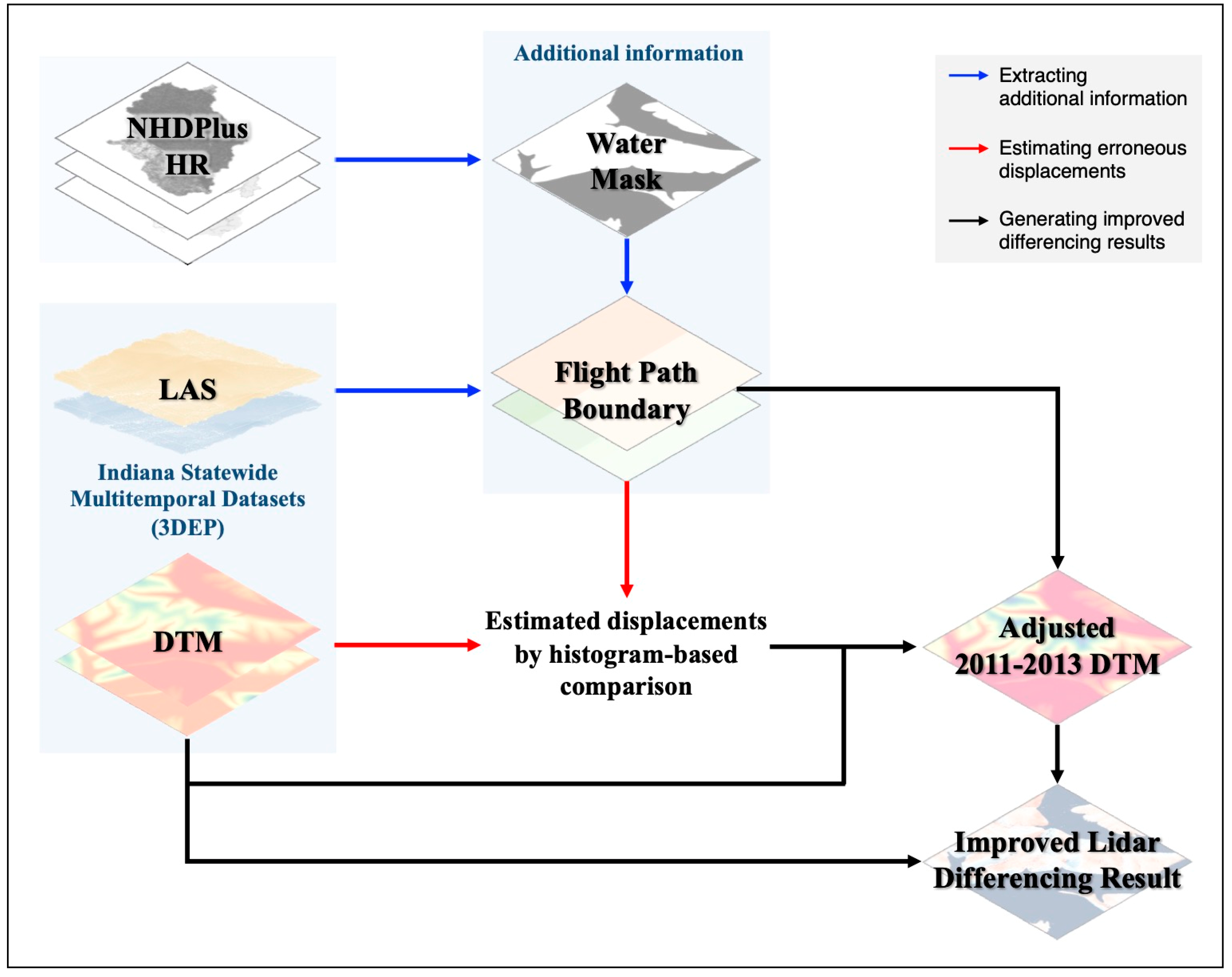
Indiana statewide topographic information has been acquired twice using an airborne lidar system from 2011 to 2013 and 2016 to 2020. The statewide lidar data provide broad insights into the challenges in processing and analyzing high-quality and large-scale multitemporal lidar data. They were collected as parts of the 3DEP, a nationwide height information collection project managed by the USGS. The 3DEP aroused expectations to facilitate many valuable downstream applications using elevation data. Several studies have derived meaningful information from 3DEP products [24,30,34] by developing and implementing appropriate approaches to overcome the difficulties of handling these large-scale datasets.
The Indiana statewide multitemporal datasets were collected over the entirety of Indiana (94,324 km2) with an average point density of 1.6 pts/m2 for the 2011–2013 dataset [24] and at least 2 pts/m2 for the 2016–2020 dataset [35]. Through a complicated and time-intensive data processing workflow, two source products, the lidar point cloud (or LASer file format, LAS) and DTM, were generated from each data collection and became available to the public in 2021 [35]. The DTM provides essential terrain heights (bare-earth, hydro-flattened, gravity-related heights) with spatial resolutions of 1.524 m (5 ft) for the 2011–2013 dataset and 0.762 m (2.5 ft) for the 2016–2020 dataset. The LAS file includes detailed information about all recorded points, such as their exact 3D position, class (e.g., ground or noise), intensity, flight path ID, and global navigation satellite system (GNSS) time. The approximate total data sizes of the LAS and DTM products are 4.9 and 0.5 terabytes for the 2011–2013 data and 13.0 and 0.7 terabytes for the 2016–2020 data. To efficiently handle these voluminous bi-temporal Indiana lidar datasets, entire areas of the individual 92 Indiana counties were divided into square grids (tiles) with a size of 1524 m by 1524 m, and the lidar products (LAS and DTM) were separately archived according to these tiles for both periods [36]. Although the geometric accuracy of each dataset has not been reported publicly in detail, the 2016–2020 dataset should meet USGS quality level 2 [37]. This implies that the absolute vertical accuracy of the root mean square error (RMSEz) is 0.1 m for non-vegetated areas, which has been announced as twice as accurate as the 2011–2013 dataset by the Indiana Geographic Information Council (IGIC) [35].
Scott et al. [24] first presented Indiana’s statewide elevation changes by designing and implementing an automatic DoD process for these big Indiana datasets. The significant topographic changes over the states, such as river fluvial changes, coastal erosion, and newly constructed roads, were effectively detected based on the DoD results. However, simultaneously, the spurious stripes along north-to-south (NS) and west-to-east (WE) directions were observed in the differenced DTM [38], making analysis of the DoD results challenging. These abnormal elevation changes were concrete evidence of the inherent errors included in Indiana datasets but have not been resolved due to a time- and labor-intensive process using flight trajectory files that have not been distributed to the public.
The striped elevation changes throughout Indiana’s statewide differencing results were likely incurred primarily by inconsistent positioning errors of the flight paths, particularly those of the 2011–2013 dataset [24]. Therefore, correcting the dissimilar 2011–2013 positioning errors can significantly reduce the problematic elevation changes in the DoD result. An ICP-based method has been applied to mitigate relative positioning errors between adjacent flight paths [39]. However, due to its iterative process, the ICP method is inefficient for the massive Indiana dataset. In addition, the ground points within the overlap areas of the 2011–2013 flight paths have not been defined in the provided LAS files. Ground point classification in the overlap areas is thus required prior to implementing the ICP-based method, which is also time-consuming.
The positioning errors can be divided into vertical and horizontal errors, which are assuredly included in the dataset. However, the vertical errors are likely more severe than the horizontal errors throughout Indiana’s DoD results. Unlike vertical errors, horizontal errors do not induce errors in the height values over plains. Contrarily, they bring out the remarkable artificial errors in slopes. Figure 1 shows examples of the county-level DoD results between the 2011–2013 and the 2016–2020 DTMs provided publicly as basic lidar products. Most of the remarkable artificial elevation changes in Figure 1 appear as long, broad stripes irrespective of the terrain slopes. Consequentially, it can be inferred that the vertical errors mainly pose difficulties in accurately analyzing the DoD results. In this respect, this paper developed a novel and practical solution for the vertical positioning errors of the 2011–2013 datasets to improve the quality of their differencing results.

3. Methodology

The proposed scalable method estimates the erroneous displacements mainly induced by dissimilar vertical positioning errors along the flight paths by comparing bi-temporal DTMs provided as source products of Indiana lidar datasets rather than time-intensive point cloud adjustment. The estimated displacement values were then utilized to adjust the 2011–2013 flight paths. Using the existing DTMs only, we developed a simple but efficient and practical method to alleviate the problematic errors in large-scale Indiana DoD results with a high degree of automation. The proposed method consists of three main steps: (1) extracting additional information for effective comparison of bi-temporal DTMs, (2) estimating the erroneous displacements between the 2011–2013 and the 2016–2020 DTMs, and (3) generating improved differencing results by adjusting the 2011–2013 DTMs, as shown in Figure 2.
This paper used the 2016–2020 DTMs as references, and the 2011–2013 DTMs were aligned with them. The advances in lidar systems have increased lidar position accuracy [40], and it was reported that the 3DEP products’ vertical accuracy have consistently increased [30]. As a result, the 2011–2013 dataset has lower vertical accuracy than the 2016–2020 dataset, and its vertical positioning errors can be reduced once aligned with the 2016–2020 dataset. Furthermore, the height values of the bi-temporal DTMs are mostly identical if there is no vertical positioning error. The Earth’s surface rarely changes evenly over a specific and broad area, especially like the striped areas of the individual 2011–2013 flight paths. Accordingly, the proposed method in this paper compared the height values of the bi-temporal DTMs using pairs of the 2011–2013 flight paths and their corresponding 2016–2020 paths, which were spatially overlapped, to examine whether they have certain artificial displacements. If the displacements were detected, they were regarded as induced by the vertical errors of the 2011–2013 flight path, and the proposed algorithm described in the following section alleviated them from the 2011–2013 DTMs. For brevity, the ‘target’ and the ‘reference’ datasets refer to the 2011–2013 and the 2016–2020 datasets for the rest of this paper. The entire process described in the following sections, except data download, was implemented using various packages with Python programming languages, such as the Geospatial Data Abstraction Library (GDAL), laspy, OpenCV, pyproj, and SciPy.

3.1. Extracting Additional Information

Because we observed a systematic striping pattern from the original DTM differencing results, we hypothesized that the striping pattern originated from issues within the individual flying strips. For this reason, we extracted additional information to effectively compare the height values from the target (2011–2013) and the reference (2016–2020) DTMs in this paper. Two different types of information were extracted from other data except for the DTMs prior to the following comparison step. One was water masks to mask out the water bodies, as lidar measurements are less reliable than ones over the ground. Hence, DTM values over the water body might show significant elevation differences between the two DTMs. The other was the boundary information of each flight path composing Indiana statewide datasets. The flight path boundary information would help independently adjust the vertical displacements of flight strips.

3.1.1. Water Mask

By the nature of the Earth’s surface, the values of the bi-temporal DTMs should be similar on a macroscale throughout the individual counties. However, some regions, like water bodies, unavoidably show significant and distinct differences between the target and the reference DTMs. As the area of the water bodies accounted for a considerable proportion of the entirety of Indiana, the water bodies could severely disrupt the comparison of the bi-temporal DTMs. Therefore, the water bodies, such as lakes, ponds, streams, and rivers, needed to be masked out during the comparison.
The water mask in each county was generated using National Hydrography Dataset Plus High Resolution (NHDPlus HR) available to the public [41]. NHDPlus HR provides valuable information on the U.S. inland waters with diverse feature classes [42]. Two classes related to the water surface, NHDArea and NHDWaterbody, were used to determine the water surface. Most NHDPlus HR products have been published on different dates according to hydrologic second-level units (or Hydrologic Unit (HU)-4 Subregion) with a scale of 1:24,000 or better. Entirety of Indiana comprised eight different HU-4 Subregions, of which the products were published in 2019 and 2020. The eight products were downloaded via USGS national map download v2.0 [41]. Indiana statewide water masks were generated by merging the two feature classes of the eight downloaded NHDPlus HR products and dividing them into the same tiles of the DTMs.

3.1.2. Flight Path Boundary Information

Because the bi-temporal datasets were compared using the flight path pairs, the spatial boundaries of the individual flight paths needed to be defined. Unfortunately, the flight path boundary has not been published as a separate product. However, instead, information about the flight paths was obtainable from the LAS files because the flight paths of both datasets were indexed by number, and the numbers were stored as point_source_id in the LAS files. The LAS files provide various information on individual points with their precise 3D coordinates, unlike the DTMs based on two-dimensional (2D) image coordinates. Therefore, the following procedure was required to define the flight path boundary by aggregating the individual multiple points’ point_source_ids of the LAS file with the DTM’s pixels.
A tiled LAS file was first imported as input data. While the imported LAS file contained numerous points from various objects, only points reflected from the ground were used to define flight path boundaries in this paper. The ground points were thus extracted based on the class information in the LAS file produced by data vendors before 3DEP data publishing. Then, an empty flight boundary data file was created as an output raster file with the same coordinate system of the tiled target DTM (1.524 m spatial resolution and 1000 pixels by 1000 pixels size), which corresponded to the imported LAS file. The output file’s pixel values were determined using the point_source_id (index flight path number) of the LAS file’s ground points located within individual pixels. The corresponding ground points for each pixel were identified by converting their horizontal 2D coordinates, x and y, into the 2D image coordinates (i.e., pixel locations), m and n, of the output file.
During this procedure, the pixels on the water bodies were assigned an invalid value using the water masks generated in the previous step. When two different flight paths occupied one pixel because of the side overlap, the most frequent index number of the existing points was assigned as the index number. Contrarily, when there was a pixel with no assigned point_source_id, the nearest neighboring pixel’s ID was assigned as the index number.

3.2. Estimating Erroneous Displacements of Target (2011–2013) DTMs

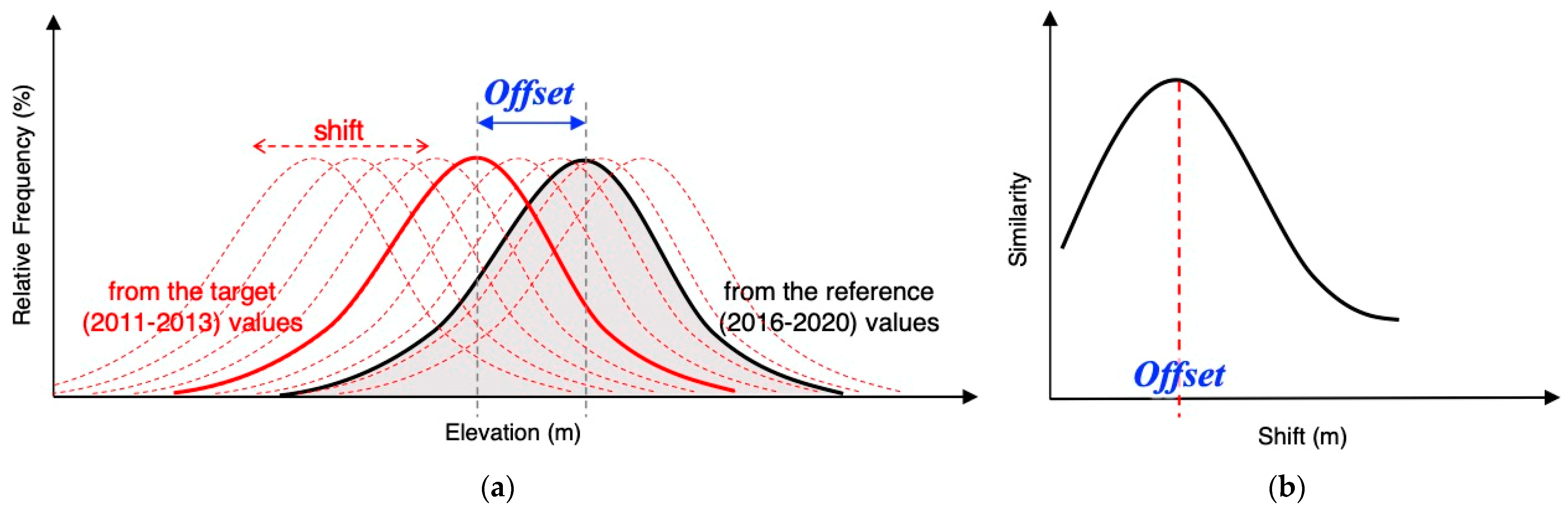
3.2.1. Gathering Height Values

Indiana’s lidar data were collected with numerous flight paths during both periods, and a single flight path covered large areas across multiple separate tiles. Therefore, the height values according to each flight path pair had to be gathered first from the multiple different tiles and then compared. Figure 3 depicts the gathering process used in this paper. Once a tiled input dataset (DTMs and flight path boundaries of two periods) was imported, the flight path pairs within the tile were defined using the flight path boundary data. For example, as illustrated in Figure 3, if there were two paths in the target data (#8–9) and three paths in the reference data (#20–22) in a tile, the four flight pairs, of which flight paths were overlapping, could be defined within the tile. These pairs were indexed as Pair (Target id, Reference id), like Pairs (#8, #20), (#8, #21), (#9, #21), and (#9, #22). According to each indexed pair, the height values of the valid pixels (i.e., non-water pixels) in target DTM and a resampled reference DTM were individually extracted and reshaped as a two-row matrix like the right of Figure 3. During the gathering process, the reference DTM was resampled using bilinear interpolation because its spatial resolution was half that of the target DTM. All the tiled DTMs in each Indiana county were sequentially processed in the same manner, and the rearranged height values from the different tiles were accumulated according to their flight path pair.

3.2.2. Histogram-Based Comparison

The long and wide spurious stripes in the original DoD results, as shown in Figure 1, revealed constant offsets between the target and the reference DTMs caused by vertical positioning errors. The offsets between the bi-temporal DTM values were estimated using the gathered height values according to the flight path pairs indexed in the previous process. In this paper, the target and the reference values were compared through their histograms to estimate offsets rather than compared pixel-by-pixel considering inevitable noises in the DTMs [43,44,45]. A histogram is a simple and effective way to describe data and has been used for many applications, including comparing multiple data, like in change detection [46] or image registration [47,48].
Figure 4 illustrates the histogram-based comparison implemented in this paper. As the area of the single flight path pair is extensive, the area where the terrain has changed generally is not broad enough to affect a histogram at a macroscale. Thus, the two histograms from the bi-temporal height values within one flight path pair are expected to be similar but have a displacement in the elevation domain induced by a constant offset due to vertical errors, as depicted with a red solid line and a black solid line in Figure 4a. To estimate this offset, the target histogram was gradually shifted by adding increasing values from −1 m to 1 m with a fixed interval of about 0.015 m (0.05 ft) to their height values, like the red histogram’s movement from left to right in Figure 4a. The similarity between the shifted target histogram and the reference histogram was calculated at every movement. When the target histograms shifted as the same offset amount, the two histograms would almost correspond, and their similarity would become the maximum value. Hence, the offset between the bi-temporal histograms could finally be determined as the shift with the maximum similarity (Figure 4b).
Numerous similarity measures exist between two histograms [49], each with advantages or disadvantages. Choosing the most appropriate measures for the compared histograms’ properties is thus essential; however, the properties of the histograms (such as their shapes) from the numerous flight path pairs over a large area are diverse depending on land covers or terrain slopes. Accordingly, we utilized five representative similarity measures between two histograms and aggregated the offsets individually determined with the five measures. The selected five measures were correlation d1, intersection d2 [50], Bhattacharyya distance d3 [51], chi-squared distance d4, and Kolmogorov–Smirnov (KS)-test d5 as follows:
d 1 = n i = 1 n h 1 i h 2 i i = 1 n h 1 i i = 1 n h 2 i n i = 1 n h 1 2 i i = 1 n h 1 i 2 n i = 1 n h 2 2 i i = 1 n h 2 i 2 ,
d 2 = i = 0 n 1 m i n h 1 i ,   h 2 i i = 0 n 1 h 2 i ,
d 3 2 = 1 i = 1 n h 1 i   h 2 i ,
d 4 2 = 1 2 i = 1 n h 1 i h 2 i 2 h 1 i + h 2 i ,
d 5 = m a x g 1 i g 2 i
where h1 and h2 indicate the two relative frequencies in bin i of the target and the reference elevation values, respectively. g1 and g2 are the cumulative relative frequencies of the two values. The number of bins for the histograms is n. In this paper, the two histograms were generated using the common bins, of which the entire range was between the minimum and the maximum of all the compared values, and the width was 0.15 m (0.5 ft), which was ten times the interval used for shifting the target values.
Correlation d1 presents a linear relationship between two data and ranges from −1 to 1. Intersection d2 calculates an overlapped rate between two histograms and ranges between 0 and 1. Since both methods quantify the similarity between two histograms, the two histograms correspond most when the calculated intersection value is closest to 1. On the contrary, the other three methods (Bhattacharyya distance d3, chi-squared distance d4, and KS test d5) measure the dissimilarity between two histograms, and the low calculated values indicate that the two histograms are similar. Bhattacharyya distance d3 ranging from 0 to 1 is related to the amount of overlap between two data, like intersection. Chi-square distance d4 and KS test d5 come from the statistics comparing the observed and the expected distributions. Chi-square distance ranges from 0 to infinity and considers the differences between small bins more important than large bins [52], as the differences are divided by the summed frequencies according to Equation (4). KS test distance is a standard nonparametric statistical test [53], ranging from 0 to 1. Accordingly, we first extracted five individual shifts with the maximum values for correlation and intersection then with the minimum values for the other measures as the offset candidates of each flight path pair. Afterward, the final offset for each pair was determined as the majority (i.e., mode) of the extracted five shifts.

3.3. Generating Improved Differencing Results

The estimated offsets for the flight path pairs were regarded as induced by the vertical errors of the target (2011–2013) flight paths and adjusted in this paper. All target DTMs with their corresponding flight path boundary data were subsequently loaded, and the adjusted target DTMs were generated by subtracting the estimated offsets from the loaded DTMs according to each flight path pair boundary.
DoD is a straightforward method compared to other lidar differencing methods once rasterized elevation products are generated from the lidar [54]. Since Indiana’s target and reference DTMs were divided into common tiles, DoD was simply implemented by subtracting the heights of the adjusted target DTMs, z t a r a d j , from the corresponding reference DTMs, z r e f r e s , which were resampled as conducted in the previous comparison step:
z d i f = z r e f r e s z t a r a d j
The elevation difference z d i f presents the terrain changes between the two periods with reduced erroneous displacements according to vertical positioning errors. The final differencing results were generated by merging all the tiled DoD results within each Indiana county.

4. Experimental Results
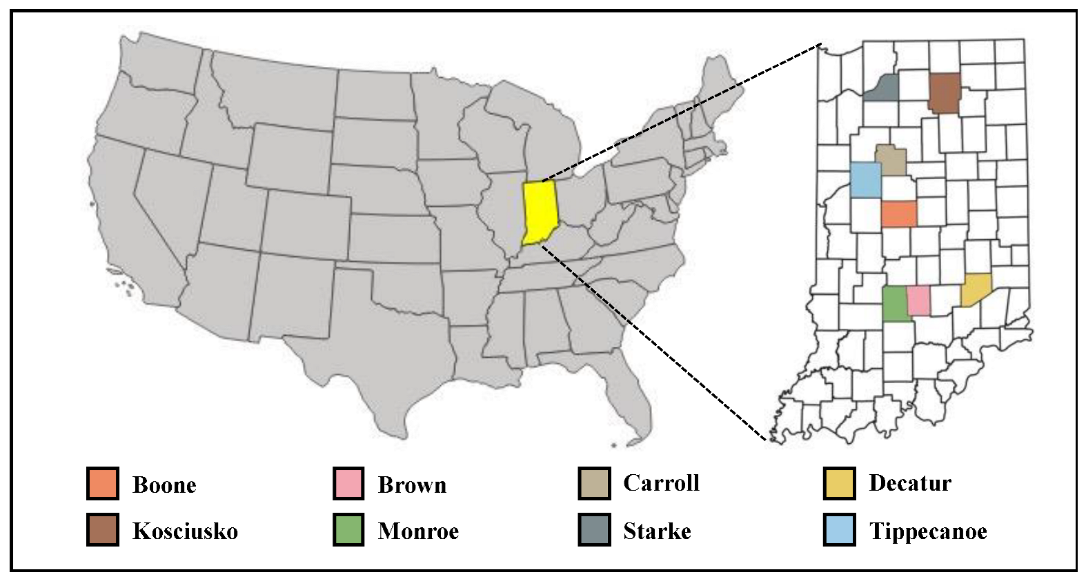
4.1. Study Sites

As Indiana’s statewide lidar products were collected and provided by counties, the proposed method was implemented on a county scale, and we assessed its feasibility and effectiveness based on the generated DoD results. A total of 8 out of 92 Indiana counties were selected as the experimental sites, representing different levels and appearances of the errors in the original DoD results (which were generated using the as-provided DTMs), as shown in Figure 1: Boone, Brown, Carroll, Decatur, Kosciusko, Monroe, Starke, and Tippecanoe. The lidar products of the eight counties were downloaded through the Integrated Digital Forestry Initiative at Purdue website [36]. The constant abnormal changes in the original DoD results clearly appear along the 2011–2013 flight paths over the selected counties. Most errors seem within the expected range of ±0.3 m based on the RMSEz values announced by the IGIC [7]. Regardless of the severity of the errors, the existence of inherent errors is manifested over the counties, which disrupts a macroscale topographic change analysis. The selected counties’ detailed specifications and locations are presented in Table 1 and Figure 5, respectively. The proposed method processed 4076 tiled datasets (bi-temporal DTMs and flight boundary data with water masks), and the height values from 6178 flight path pairs were gathered and compared throughout the 8377 km2 study sites, which are sufficient for evaluating the proposed method’s scalability (i.e., feasibility and effectiveness) for a large-scale 3DEP dataset.

4.2. Effectiveness of Proposed Method

This paper developed a new method to reduce the artificial displacements along the flight paths observed throughout the differencing results. However, the appropriate reference data, which enabled quantifying the individual flight path’s accuracy over Indiana, was absent. As an alternative, the proposed method’s results, (1) the displacements estimated with the histogram-based comparison and (2) the adjusted DoD results, were compared with the original DoD results in Figure 1.

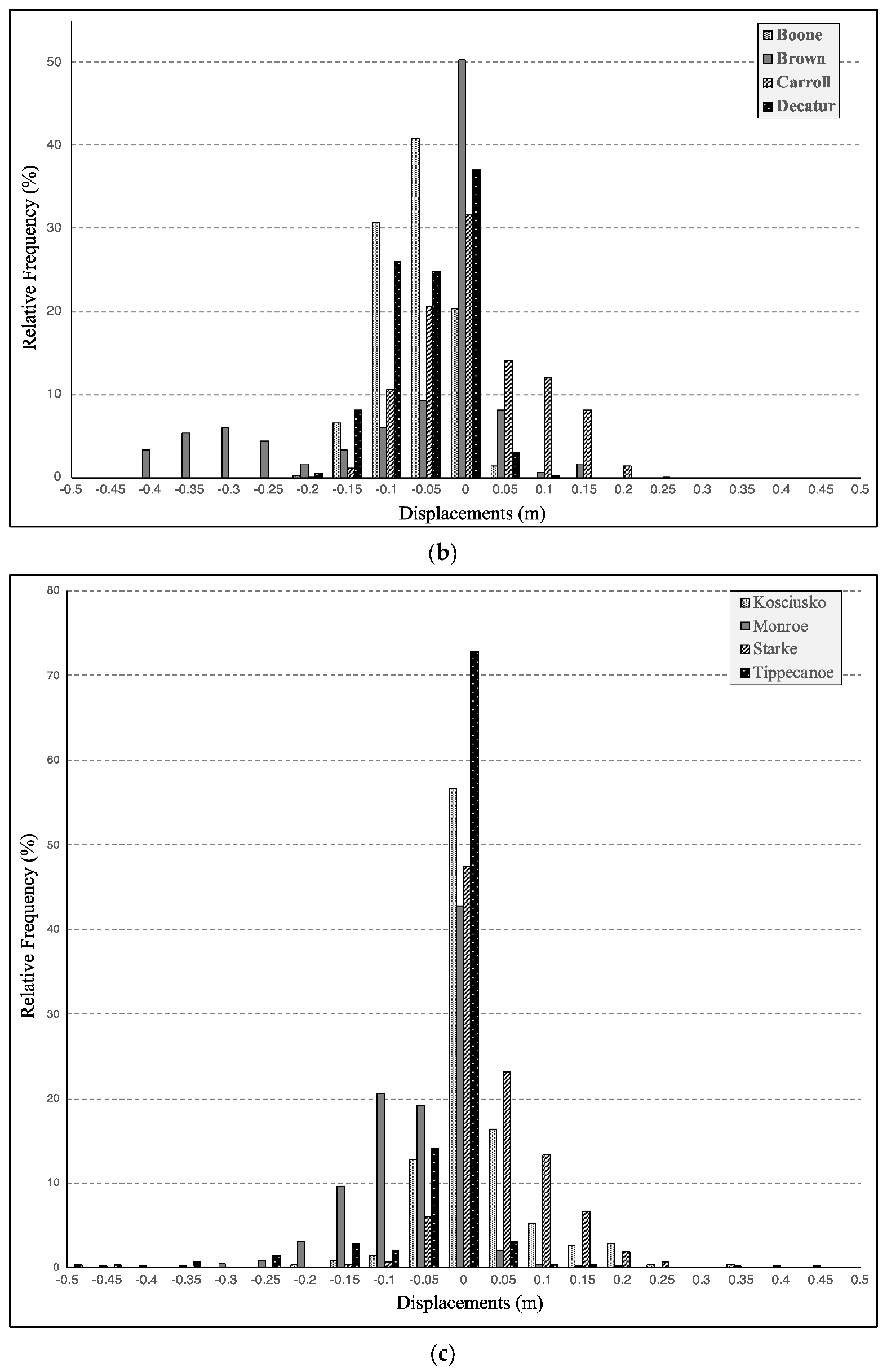
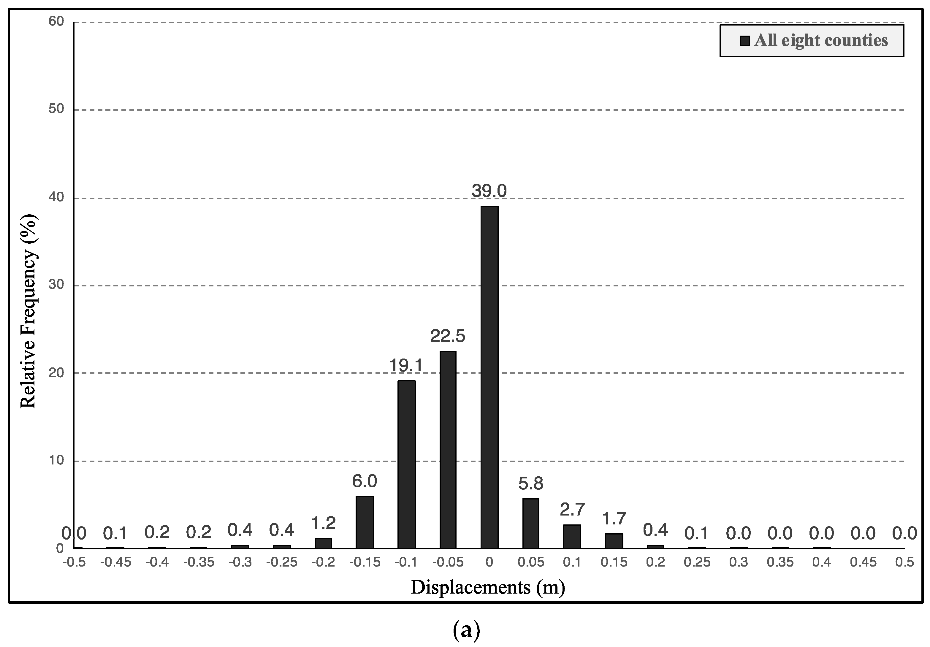
4.2.1. Estimated Displacements by Vertical Positioning Errors

The original DoD results in Figure 1 revealed the existence of the inherent vertical errors in the Indiana datasets, but the severity of the errors could not be quantitatively measured. In this respect, we investigated whether the estimated displacements from the proposed histogram-based comparison could quantitively represent the errors displayed in Figure 1. Table 2 summarizes the range of each county’s estimated displacements based on its 5 and 95 percentile values. The county-level estimated displacements range between −0.345 m and 0.147 m. Specifically, 39.0% of the eight counties’ total flight path pairs were determined to include minimal displacements with absolute values of less than 0.025 m according to Figure 6a, which is the relative frequency histogram of the entire flight path pairs’ estimated displacements. The additional 57.8% of pairs contained absolute vertical displacements less than 0.15 m. These estimated values agreed with the expected range based on the RMSEz announced by the IGIC [35] as well as the visually observed ranges based on the original DoD results in Figure 1.
The estimated errors of each county are also demonstrated to be consistent with the problematic elevation changes found in the original DoD results (Figure 1). The relative frequency histograms of each county’s estimated displacements are presented in Figure 6b,c. For instance, according to Boone County’s histogram in Figure 6b, over 70% of the displacements were estimated between −0.10 and −0.05 m. These estimations were considered reasonable compared to Boone County’s original DoD results, doubtfully indicating that the terrain commonly increased throughout the county. Similarly, the displacements of the other counties, where the elevations appeared generally and evenly increasing or decreasing in their DoD results, seemed as adequately estimated by the proposed method according to their histograms.
One noteworthy county is Brown County, which had the most severe errors in the original differencing results among the eight counties, as demonstrated in Figure 1. The more significant number of Brown County’s flight path pairs had displacements around −0.3 m (Figure 6b), which appeared as the distinct blue regions in Figure 1, compared to those of other counties. Furthermore, its histogram is demonstrated to consist of two distinguished distributions concentrated around −0.3 m and 0 m, which could also be visually identified in the original DoD results. In contrast, Tippecanoe County was presented to have the least errors according to the DoD results (Figure 1) and the estimated displacements by the proposed method. Figure 6c exhibits that a large number (72.9%) of Tippecanoe County’s flight path pairs have minimal displacements with absolute values of less than 0.025 m. Such consistency in the estimated displacements’ ranges (Table 1) and distributions (Figure 6) with the visual inspection results of the original DoD results (Figure 1) demonstrates that the proposed histogram-based comparison could quantitatively measure the vertical-error-induced displacements in the DoD results. Consequentially, it can be expected that the problematic striped errors will be reduced significantly in the differencing results presented in the following section by adjusting these properly estimated erroneous displacements.

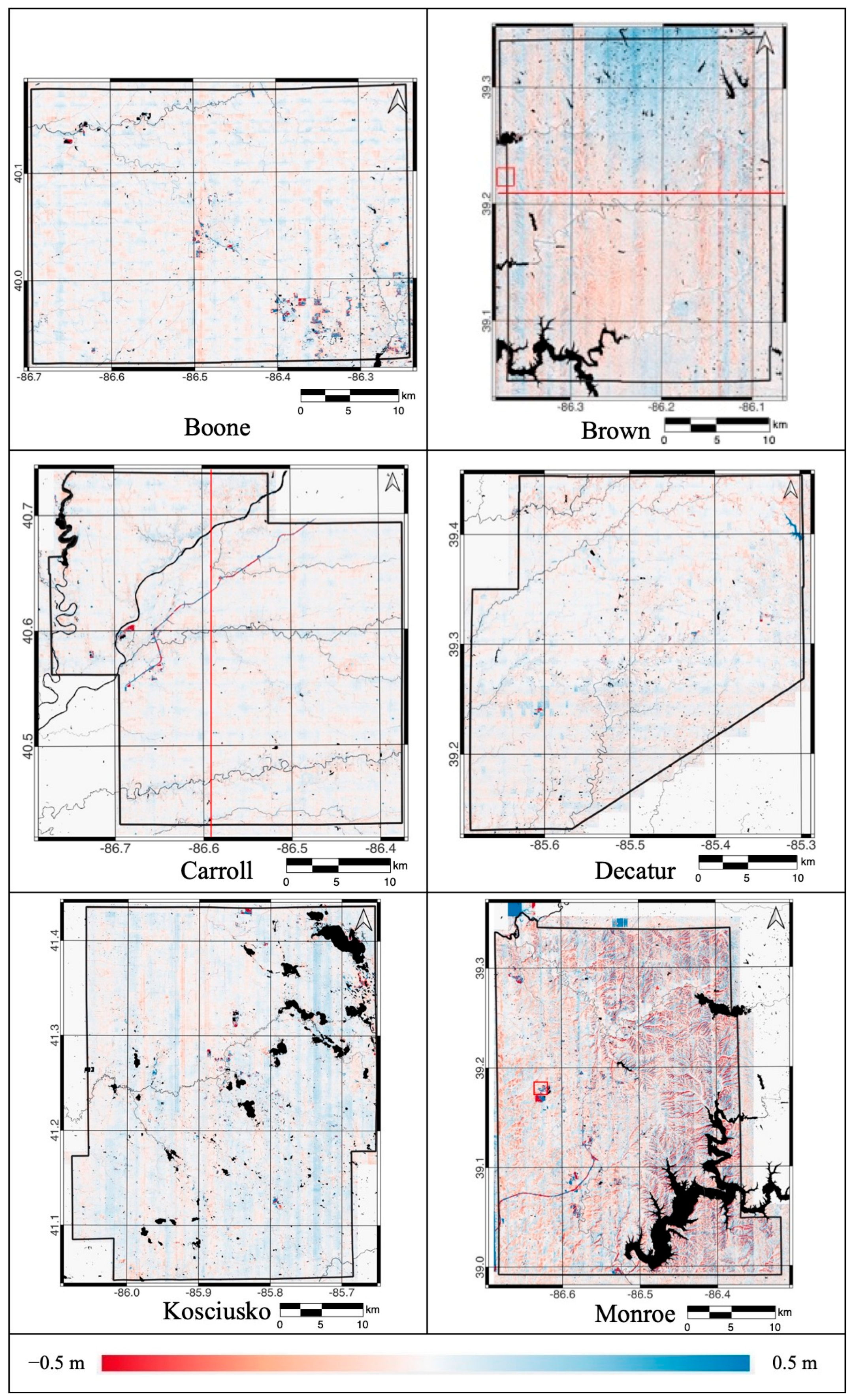
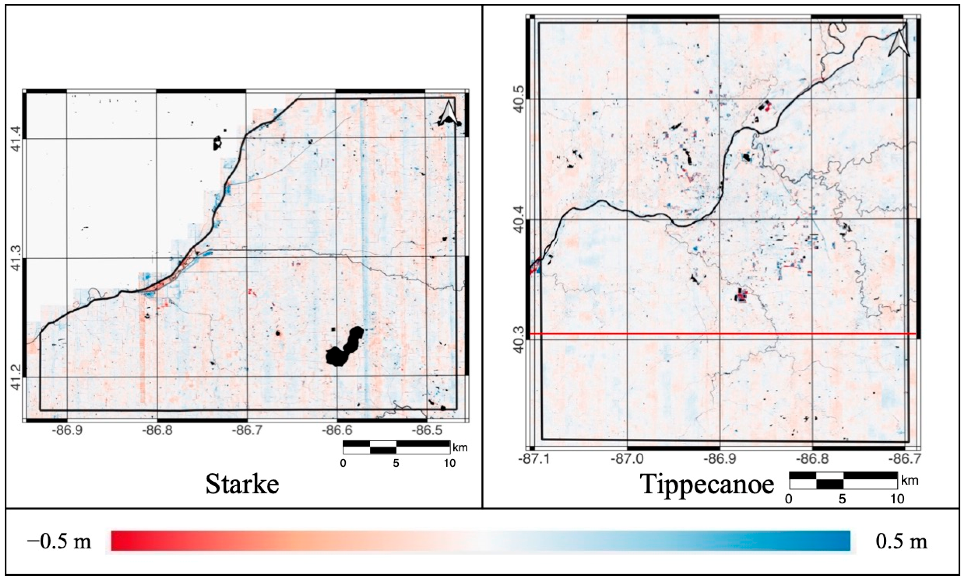
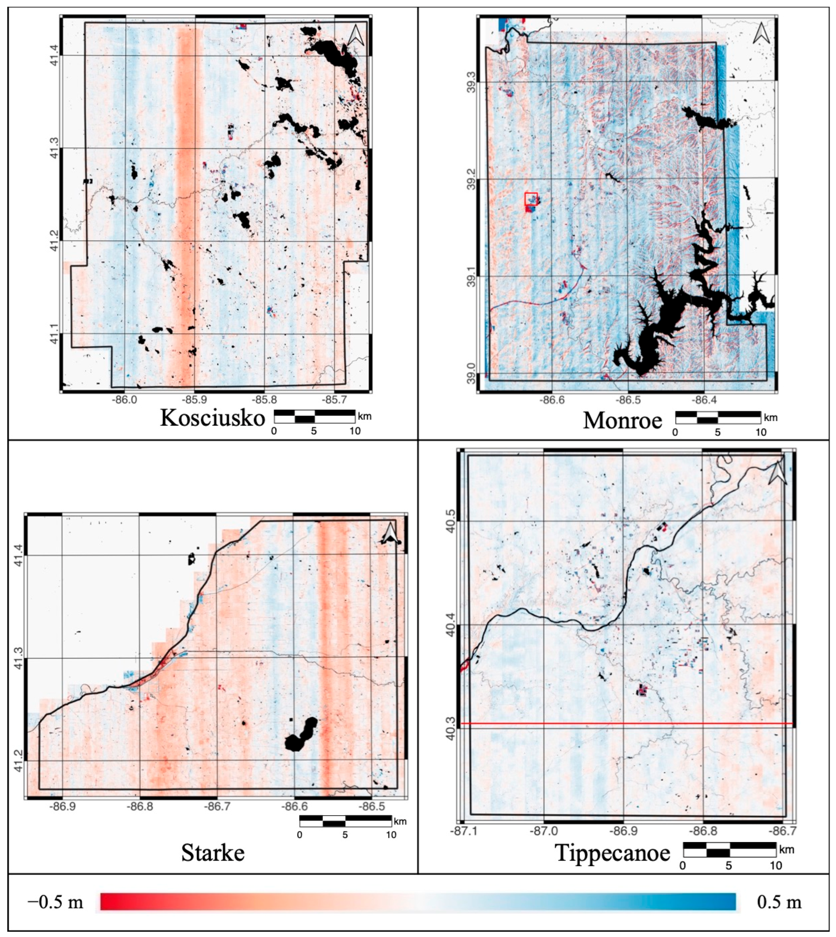
4.2.2. Improved County-Level DoD Results

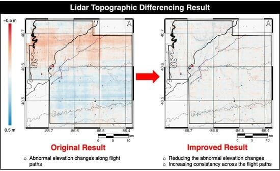
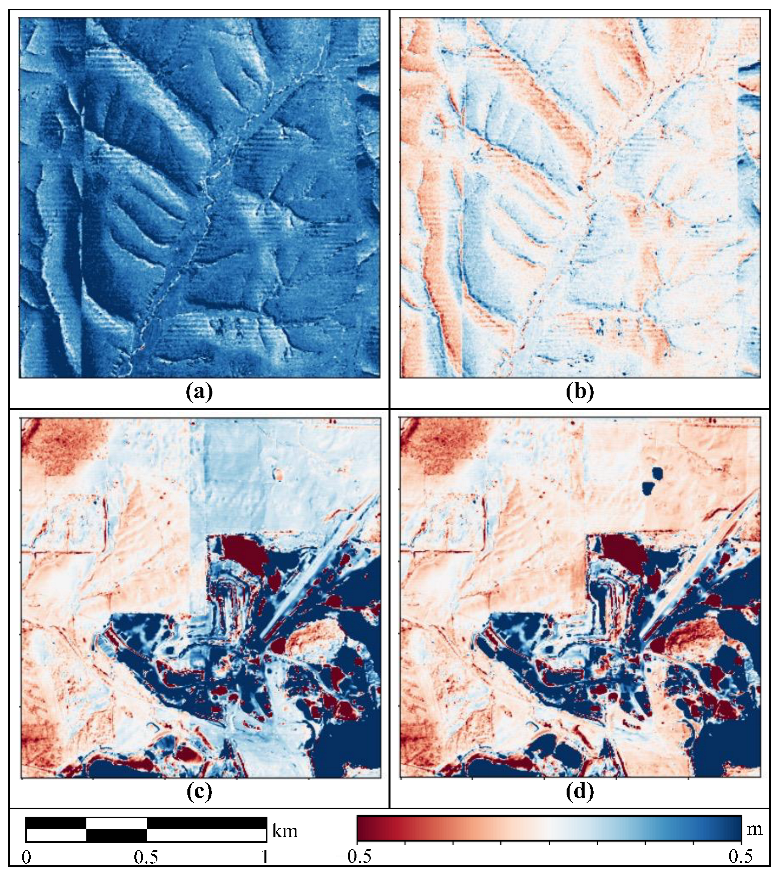
  • Comparison on a county-level scale
The target (2011–2013) DTMs were adjusted using the estimated displacements, and the adjusted DoD results were finally generated. Figure 7 presents the thumbnail images of the adjusted county-level DoD results. The results demonstrate a higher consistency throughout the counties with fewer abnormal striped changes than the original DoD results in Figure 1. Even though the vertical error within each flight path pair was modeled as one constant value (i.e., offset) in this paper, the DoD results in Figure 7 reveal that the proposed method is effective overall in the eight counties regardless of the errors’ severities or patterns.
To quantitatively compare the original and the adjusted county-level DoD results, we calculated and compared the median values of the individual 2011–2013 flight paths for both DoD results. A common 2011–2013 flight path area is a stripe of several tens of kilometers by more than 1 km, including up to twenty million pixels of the DoD results. Even though the terrain heights changed within several regions during the data collection periods, the changes likely randomly occurred over small areas, and thus the terrain height could be regarded as stable overall in this massive flight path area. As a result, the calculated medians of the DoD values within each 2011–2013 flight path should be near zero unless there are systematic vertical errors within the paths, and we can measure the level of abnormal elevation changes in the DoD results by analyzing the median values.
The calculated medians within each county were analyzed using their absolute mean and standard deviations, as summarized in Table 3. It is noticed that the absolute means and the level of the abnormal elevation changes are related by comparing the absolute means in Table 3 and the county-level DoD results in Figure 1 and Figure 7; as the absolute mean value increased, the more abnormal changes were observed in the DoD results. For example, Carroll County, with the lowest absolute mean (0.0023 m) among the values in Table 3, appeared as the adjusted DoD result with the least abnormal elevation changes in Figure 7. Boone and Decatur Counties, which have similar absolute mean values to that of Carroll County, also present comparably fewer abnormal elevation changes in their adjusted DoD results. In contrast, the counties with high levels of systematic errors in their adjusted DoD results (Figure 7), such as Brown and Monroe Counties, show about ten times higher absolute mean values of 0.0240 m and 0.0210 m (Table 3), respectively, than that of Carroll County. As a result, based on this relationship, we can quantitatively assess the proposed method’s effectiveness by calculating a relative decrease in the absolute means between the original and adjusted DoD results. Equation (7) shows an improvement ratio R used to measure the relative decrease in this paper.
R = ( m 1 m 2 ) m 1 × 100
where m1 and m2 are the absolute means of the original and the adjusted DoD medians, respectively.
The R values in Table 3 illustrate the effectiveness of the proposed method in this paper to reduce the abnormal elevation changes in the original DoD results. The high R values of more than 50% in Table 3 illustrate that the medians of the DoD values within the individual flight paths became close to zero as the proposed method mitigated the possible abnormal elevation changes. In addition, the decrease in the standard deviation of the median values in the adjusted DoD results for each county (Table 3) can be interpreted as the consistency between the adjacent flight paths increasing, as visually identified in Figure 7. Meanwhile, the different R values of the eight counties imply that the proposed method was inevitably affected by inherent problems in the large datasets, such as irregularly overlapped areas of the 2011–2013 and the 2016–2020 flight paths, errors in the water masks induced by the temporal differences between the NHDPlus HR datasets and bi-temporal Indiana datasets, and errors in the point_source_id of the provided LAS files. Nevertheless, the decreases in their absolute means and standard deviations in Table 3 quantitatively present the proposed method’s effects in reducing the errors along the flight paths observed in the original DoD results, as shown in Figure 7.
  • Detailed comparison with examples
For further investigation of the improvements due to the proposed method, the original and the adjusted DoD results were compared based on their profiles (or cross-sections). The profiles of the representative three counties’ DoD results were extracted, as shown in Figure 8. Brown, Carroll, and Tippecanoe Counties were selected as the representatives for the large errors, the moderate errors, and the small errors, respectively, considering the diversity of the error levels and patterns. The locations of the profiles were randomly selected, and their directions were determined perpendicular to the 2011–2013 flight paths. Due to the inherent random noises of the DTMs, the profile values were extracted by averaging 10 pixels by 10 pixels (i.e., 15.24 m or 50 ft).
Figure 8. Profiles (cross-section) of the three representative counties’ DoD results: (a) Brown County in the west-to-east (WE) direction; (b) Carroll County in the north-to-south (NS) direction; and (c) Tippecanoe County in the WE direction. The trace for each profile is presented as red lines in Figure 1 and Figure 7. The profiles were extracted based on the average values of every 10 pixels by 10 pixels (i.e., 15.24 m or 50 ft) area. The black and red lines indicate the values of the original and the adjusted DoD results, respectively. The blue dotted lines indicate the boundaries between the adjacent 2011–2013 flight paths, and the grey lines present theoretically ideal elevation changes at the macroscale (i.e., where the DoD value is 0). Some conspicuous values were actual elevation changes or the water bodies, which are not removed with NHDPlus HR.
Remotesensing 15 04289 g008aRemotesensing 15 04289 g008b
The profiles again revealed that the proposed method reduced the abnormal elevation changes due to the inherent vertical errors along the flight paths. The original DoD results’ profiles (the black lines in Figure 8) illustrate the two typical problematic elevation changes visually identified in Figure 1. One is the consistently positive or negative average DoD values throughout the multiple flight paths presented over several kilometers across the flight paths in Brown and Carroll Counties’ profiles (Figure 8a,b). The most obvious identified erroneous changes are observed in the western and eastern regions of Brown County, and their widths are about 8 km. The other problematic change is a discontinuity between adjacent flight paths, such as sudden dramatic rises or falls between the adjacent flight paths, as seen in Figure 8a. Such problems possibly result in misinterpretation of the actual county-level topography changes.
These problems were mitigated in the adjusted DoD results, as demonstrated with the red profiles in Figure 8. As the vertical erroneous displacements decreased with the proposed method, the profiles along several tens of kilometers were aligned to 0 m, which were considered reasonable elevation changes on a macroscale. In addition, the profiles became more consistent along the WE or NS directions across the flight paths. Simultaneously, it was found that the variations of the elevation changes within the individual flight paths were unaffected by the proposed method. This indicates that meaningful elevation changes can still be easily observed in the adjusted DoD results.
The findings from the profiles are also observed in the tile-size DoD results (1524 m by 1524 m), as shown in the examples in Figure 9. Figure 9a shows the unrealistic elevation changes, as the entire area had evenly risen over 0.3 m between 2011–2013 and 2016–2020. Figure 9c illustrates a distinct artificial line in the middle of the tile induced by the discontinuity between the adjacent flight paths. Through the examples, it is predictable that such problematic changes in the original DoD results will bring an inaccurate terrain change analysis. The proposed method alleviated these abnormal changes, and thus more reasonable DoD results were created, as shown in Figure 9b,d. Furthermore, the detailed elevation changes in the overall areas are maintained in the adjusted DoD results. Therefore, the meaningful elevation changes in Figure 9d are expected to be analyzed more accurately as having less discrepancy between the adjacent flight paths.
Figure 9. Examples of the tile-size DoD results. (a,c): the original tiled DoD results. (b,d): the adjusted tiled DoD results. (a,b) are mountainous areas in Brown County, and (c,d) are near a quarry in Monroe County. The exact locations are marked as red boxes in Figure 1 and Figure 7.
Remotesensing 15 04289 g009
To complement the missing appropriate reference data for assessment, we comprehensively compared the original and our adjusted DoD results using the flight path median values, the county-level profiles, and the tile-level examples. Through three different assessments, it was consistently demonstrated that the proposed method could considerably reduce the apparent problems in the original lidar differencing results, and the adjusted differencing results generated in this paper could provide more reasonable information about the elevation changes in eight county-level study sites. Given that its effectiveness was validated over large 8377 km2 study sites composed of 6178 flight path pairs (Table 1), the proposed method is expected to be scalable as well as universally applicable for various levels and patterns of errors over different land covers. Furthermore, the proposed method can be implemented automatically once additional data regarding the water bodies is prepared, which is often available to the public [55,56], including the NHDPlus HR. Although few parameters were required for histogram-based comparison, the advanced quality differencing results were generated without changing them throughout the experiments in this study. Consequentially, we expect the proposed method to be a feasible solution to mitigate the apparent errors in multitemporal lidar datasets expectedly collected given the recent active government-driven lidar data acquisition without a time-intensive process.

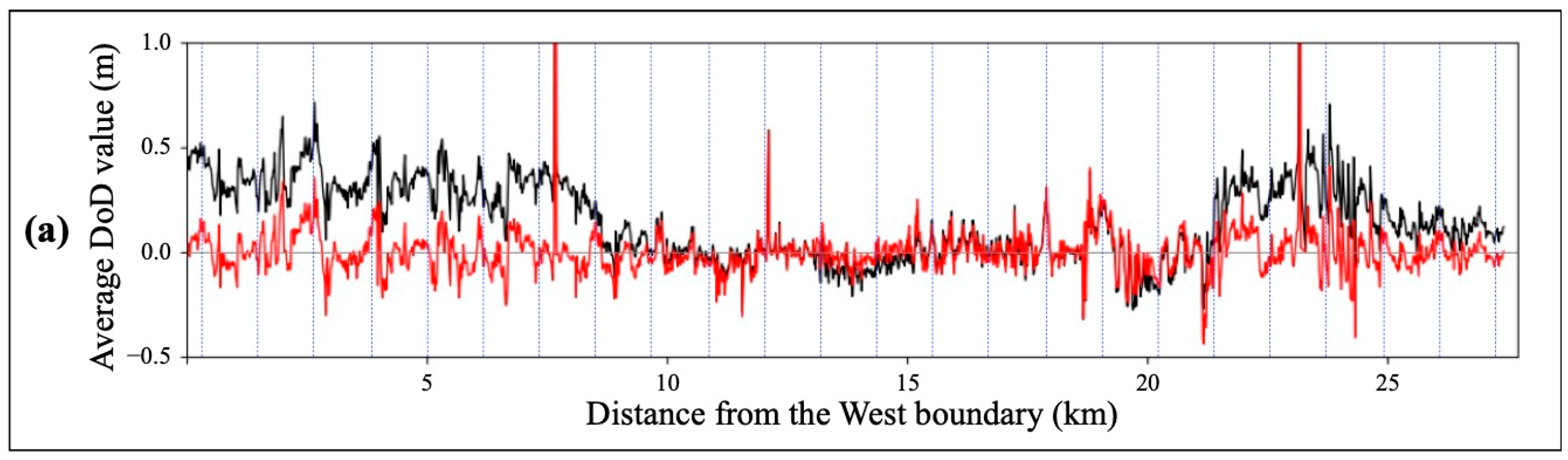
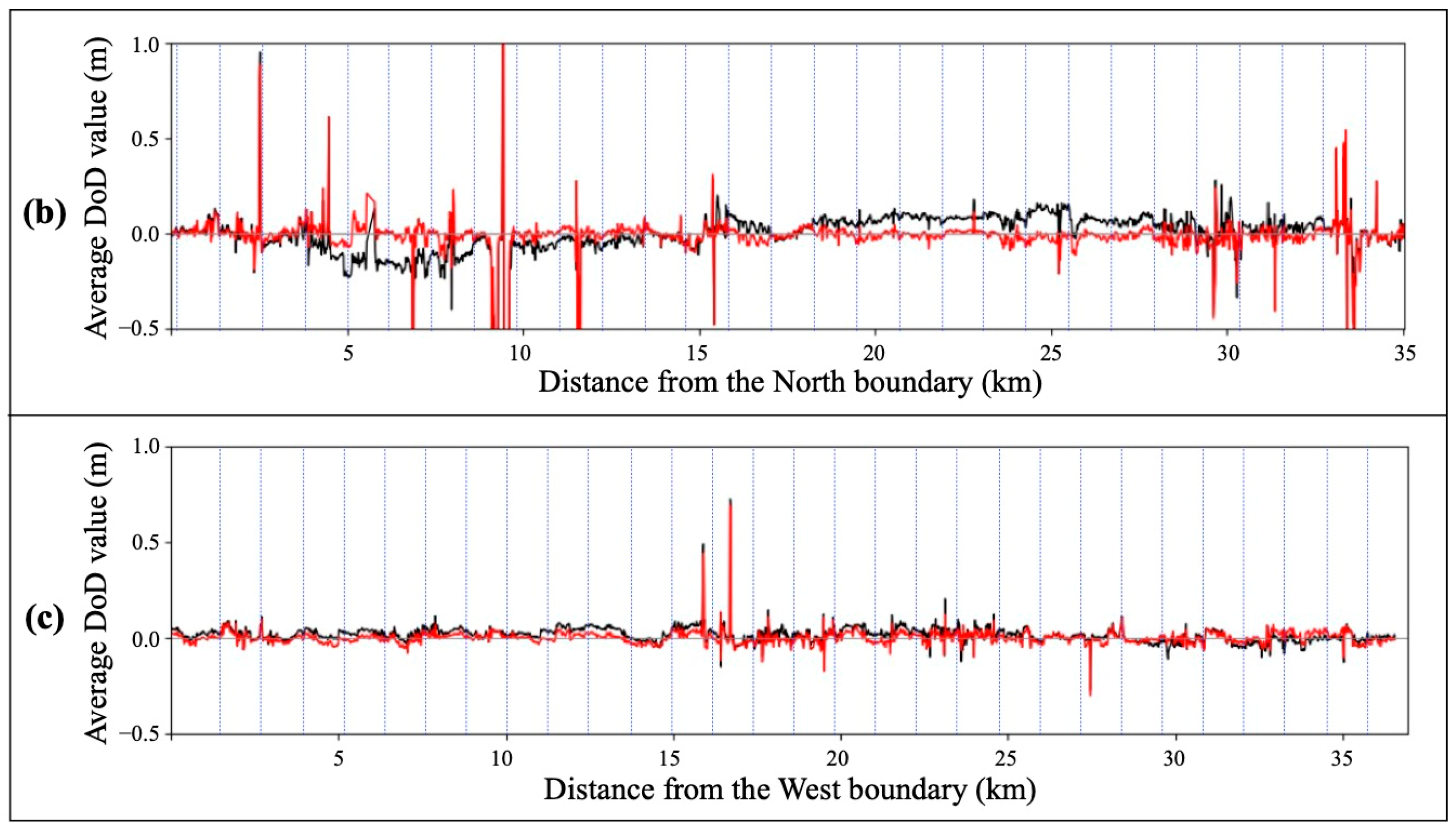
4.3. Remaining Horizontal Positioning Errors

Although the proposed method was effective against critical vertical positioning errors, minor abnormal changes caused by the other error sources inevitably remained. One representative remaining error source is the horizontal positioning error. The horizontal error does not cause an apparent problem in plains. Still, it may become a problem in slopes because terrain aspects and slopes determine the sign and magnitude of the abnormal changes caused by horizontal errors. Figure 9b demonstrates the inherent horizontal errors over a mountainous area of Brown County. The opposite elevation differences in the opposite aspect, as shown in Figure 9b, are the visual evidence of the horizontal positioning errors in the dataset. In this respect, the counties with steep hills or mountains, such as Brown and Monroe Counties, have prominent remaining abnormal elevation changes in the adjusted DoD results (Figure 7) compared to the other relatively plain counties.
It would be ideal that the horizontal errors could also be reduced with simple implementation. However, it seems nearly impossible to adjust the horizontal errors using the provided DTM, like the proposed method in this paper, because the horizontal errors in Indiana datasets are predicted to be less than the provided DTM’s spatial resolution of 1.524 m (5 ft). Precise processing of low-level point cloud data, like a conventional method appropriate for a microscale, is inevitably required to achieve an accurate terrain change analysis over the mountain areas. Therefore, solving the horizontal errors is out of the scope of this study, which was developing a feasible method for a massive lidar dataset, and we would like to handle this problem in a future study.

5. Conclusions

Considering the previous methods’ practical limitations, this paper has presented a scalable method to mitigate the spurious elevation changes in large-scale multitemporal lidar differencing results. The proposed method focused on resolving critical vertical positioning errors by comparing bi-temporal DTMs readily provided as basic lidar products. By using the existing DTMs, implementing the proposed method became simple and feasible for a massive lidar dataset. The proposed method was applied to reduce the reported but unsolved abnormal changes in the DoD results of massive Indiana multitemporal 3DEP datasets [24]. The improved county-level DoD results from the proposed method were comprehensively compared with the original DoD results on macro- and microscales to complement the absent reference data. The proposed method’s effectiveness was demonstrated as (1) significantly reducing the vertical-error-induced abnormal elevation changes, (2) improving the consistency across the flight paths, and (3) simultaneously preserving details of the actual elevation changes within the individual flight paths. The remaining horizontal-induced displacements in the DoD results, which are out of the scope of this study, will be handled in a future study. The proposed method can be automatically implemented and universally applied with easily accessible water body information. Moreover, the improved Indiana lidar topographic differencing results produced in this paper are expected to facilitate more accurate and efficient downstream applications. Given the continuously increasing amount of high-quality lidar data, the proposed method can be a practical solution against the apparent errors in lidar differencing results that disturb the accurate and systematic analysis of macroscale elevation changes.

Author Contributions

Conceptualization, M.J. and J.J.; methodology, M.J. and J.J.; validation, M.J. and J.J.; formal analysis, M.J.; investigation, M.J.; resources, J.J.; data curation, M.J.; writing—original draft preparation, M.J.; writing—review and editing, M.J. and J.J.; visualization, M.J.; supervision, J.J.; project administration, J.J.; funding acquisition, J.J. All authors have read and agreed to the published version of the manuscript.

Funding

This research was supported by the Institute for Digital Forestry at Purdue University.

Data Availability Statement

Publicly available datasets were analyzed in this study. Indiana Statewide Multitemporal Lidar Datasets can be found here: https://lidar.digitalforestry.org (accessed on 15 July 2022). The National Hydrography Dataset Plus High Resolution (NHDPlus HR) can be found here: https://apps.nationalmap.gov/downloader (accessed on 4 February 2023).

Conflicts of Interest

The authors declare no conflict of interest.

References

  1. Wheaton, J.M.; Brasington, J.; Darby, S.E.; Sear, D.A. Accounting for uncertainty in DEMs from repeat topographic surveys: Improved sediment budgets. Earth Surf. Process. Landf. 2010, 35, 136–156. [Google Scholar] [CrossRef]
  2. Hooper, A.; Bekaert, D.; Spaans, K.; Arıkan, M. Recent advances in SAR interferometry time series analysis for measuring crustal deformation. Tectonophysics 2012, 514, 1–13. [Google Scholar] [CrossRef]
  3. Brozzetti, F.; Mondini, A.C.; Pauselli, C.; Mancinelli, P.; Cirillo, D.; Guzzetti, F.; Lavecchia, G. Mainshock anticipated by intra-sequence ground deformations: Insights from multiscale field and SAR interferometric measurements. Geosciences 2020, 10, 186. [Google Scholar] [CrossRef]
  4. Eltner, A.; Baumgart, P. Accuracy constraints of terrestrial Lidar data for soil erosion measurement: Application to a Mediterranean field plot. Geomorphology 2015, 245, 243–254. [Google Scholar] [CrossRef]
  5. Jones, L.; Hobbs, P. The application of terrestrial LiDAR for geohazard mapping, monitoring and modelling in the British Geological Survey. Remote Sens. 2021, 13, 395. [Google Scholar] [CrossRef]
  6. Joerg, P.C.; Morsdorf, F.; Zemp, M. Uncertainty assessment of multi-temporal airborne laser scanning data: A case study on an Alpine glacier. Remote Sens. Environ. 2012, 127, 118–129. [Google Scholar] [CrossRef]
  7. Oskin, M.E.; Arrowsmith, J.R.; Corona, A.H.; Elliott, A.J.; Fletcher, J.M.; Fielding, E.J.; Gold, P.O.; Garcia, J.J.G.; Hudnut, K.W.; Liu-Zeng, J.; et al. Near-field deformation from the El Mayor–Cucapah earthquake revealed by differential LIDAR. Science 2012, 335, 702–705. [Google Scholar] [CrossRef]
  8. Clark, K.J.; Nissen, E.K.; Howarth, J.D.; Hamling, I.J.; Mountjoy, J.J.; Ries, W.F.; Jones, K.; Goldstein, S.; Cochran, U.A.; Villamor, P.; et al. Highly variable coastal deformation in the 2016 Mw7. 8 Kaikōura earthquake reflects rupture complexity along a transpressional plate boundary. Earth Planet. Sci. Lett. 2017, 474, 334–344. [Google Scholar] [CrossRef]
  9. Ghuffar, S. DEM generation from multi satellite PlanetScope imagery. Remote Sens. 2018, 10, 1462. [Google Scholar] [CrossRef]
  10. Virtanen, J.P.; Kukko, A.; Kaartinen, H.; Jaakkola, A.; Turppa, T.; Hyyppä, H.; Hyyppä, J. Nationwide point cloud—The future topographic core data. ISPRS Int. J. GeoInf. 2017, 6, 243. [Google Scholar] [CrossRef]
  11. Li, X.; Liu, C.; Wang, Z.; Xie, X.; Li, D.; Xu, L. Airborne LiDAR: State-of-the-art of system design, technology and application. Meas. Sci. Technol. 2021, 32, 032002. [Google Scholar] [CrossRef]
  12. Chen, R.F.; Chang, K.J.; Angelier, J.; Chan, Y.C.; Deffontaines, B.; Lee, C.T.; Lin, M.L. Topographical changes revealed by high-resolution airborne LiDAR data: The 1999 Tsaoling landslide induced by the Chi–Chi earthquake. Eng. Geol. 2006, 88, 160–172. [Google Scholar] [CrossRef]
  13. Favalli, M.; Fornaciai, A.; Mazzarini, F.; Harris, A.; Neri, M.; Behncke, B.; Pareschi, M.T.; Tarquini, S.; Boschi, E. Evolution of an active lava flow field using a multitemporal LIDAR acquisition. J. Geophys. Res. 2010, 115, B11203. [Google Scholar] [CrossRef]
  14. Glennie, C.; Hinojosa-Corona, A.; Nissen, E.; Kusari, A.; Oskin, M.; Arrowsmith, J.; Borsa, A. Optimization of legacy lidar data sets for measuring near-field earthquake displacement. Geophys. Res. Lett. 2014, 41, 3494–3501. [Google Scholar] [CrossRef]
  15. Wagner, W.; Lague, D.; Mohrig, D.; Passalacqua, P.; Shaw, J.; Moffett, K. Elevation change and stability on a prograding delta. Geophys. Res. Lett. 2017, 44, 1786–1794. [Google Scholar] [CrossRef]
  16. DeLong, S.B.; Hammer, M.N.; Engle, Z.T.; Richard, E.M.; Breckenridge, A.J.; Gran, K.B.; Jennings, C.E.; Jalobeanu, A. Regional-scale landscape response to an extreme precipitation event from repeat lidar and object-based image analysis. Earth Space Sci. 2022, 9, e2022EA002420. [Google Scholar] [CrossRef]
  17. Entwistle, N.; Heritage, G.; Milan, D. Recent remote sensing applications for hydro and morphodynamic monitoring and modelling. Earth Surf. Process. Landf. 2018, 43, 2283–2291. [Google Scholar] [CrossRef]
  18. Okyay, U.; Telling, J.; Glennie, C.L.; Dietrich, W.E. Airborne lidar change detection: An overview of Earth sciences applications. Earth Sci. Rev. 2019, 198, 102929. [Google Scholar] [CrossRef]
  19. Zhong, C.; Liu, Y.; Gao, P.; Chen, W.; Li, H.; Hou, Y.; Nuremanguli, T.; Ma, H. Landslide mapping with remote sensing: Challenges and opportunities. Int. J. Remote Sens. 2020, 41, 1555–1581. [Google Scholar] [CrossRef]
  20. Chen, Z.; Gao, B.; Devereux, B. State-of-the-art: DTM generation using airborne lidar data. Sensors 2017, 17, 150. [Google Scholar] [CrossRef]
  21. Mitasova, H.; Drake, T.G.; Bernstein, D.; Harmon, R.S. Quantifying rapid changes in coastal topography using modern mapping techniques and geographic information system. Environ. Eng. Geosci. 2004, 10, 1–11. [Google Scholar] [CrossRef]
  22. Anderson, S.; Pitlick, J. Using repeat lidar to estimate sediment transport in a steep stream. J. Geophys. Res. Earth Surf. 2014, 119, 621–643. [Google Scholar] [CrossRef]
  23. Mora, O.E.; Lenzano, M.G.; Toth, C.K.; Grejner-Brzezinska, D.A.; Fayne, J.V. Landslide change detection based on multi-temporal Airborne LiDAR-derived DEMs. Geosciences 2018, 8, 23. [Google Scholar] [CrossRef]
  24. Scott, C.P.; Beckley, M.; Phan, M.; Zawacki, E.; Crosby, C.; Nandigam, V.; Arrowsmith, R. Statewide USGS 3DEP lidar topographic differencing applied to Indiana, USA. Remote Sens. 2022, 14, 847. [Google Scholar] [CrossRef]
  25. Favalli, M.; Fornaciai, A.; Pareschi, M.T. LIDAR strip adjustment: Application to volcanic areas. Geomorphology 2009, 111, 123–135. [Google Scholar] [CrossRef]
  26. What Is 3DEP? Available online: https://www.usgs.gov/3d-elevation-program/what-3dep (accessed on 15 July 2022).
  27. Besl, P.J.; McKay, N.D. Method for registration of 3-D shapes. In Proceedings of the Sensor Fusion IV: Control Paradigms and Data Structures, Boston, MA, USA, 12–15 November 1991. [Google Scholar] [CrossRef]
  28. Lallias-Tacon, S.; Liébault, F.; Piégay, H. Step by step error assessment in braided river sediment budget using airborne LiDAR data. Geomorphology 2014, 214, 307–323. [Google Scholar] [CrossRef]
  29. Nilsson, M.; Nordkvist, K.; Jonzén, J.; Lindgren, N.; Axensten, P.; Wallerman, J.; Egberth, M.; Larsson, S.; Nilsson, L.; Eriksson, J.; et al. A nationwide forest attribute map of Sweden predicted using airborne laser scanning data and field data from the National Forest Inventory. Remote Sens. Environ. 2017, 194, 447–454. [Google Scholar] [CrossRef]
  30. Stoker, J.; Miller, B. The accuracy and consistency of 3d elevation program data: A systematic analysis. Remote Sens. 2022, 14, 940. [Google Scholar] [CrossRef]
  31. Cserép, M.; Lindenbergh, R. Distributed processing of Dutch AHN laser altimetry changes of the built-up area. Int. J. Appl. Earth Obs. Geoinf. 2023, 116, 103174. [Google Scholar] [CrossRef]
  32. Chen, C.; Li, Y. A fast global interpolation method for digital terrain model generation from large LiDAR-derived data. Remote Sens. 2019, 11, 1324. [Google Scholar] [CrossRef]
  33. Aljumaily, H.; Laefer, D.F.; Cuadra, D.; Velasco, M. Voxel change: Big data–based change detection for aerial urban LiDAR of unequal densities. J. Surv. Eng. 2021, 147, 04021023. [Google Scholar] [CrossRef]
  34. Oh, S.; Jung, J.; Shao, G.; Shao, G.; Gallion, J.; Fei, S. High-resolution canopy height model generation and validation using USGS 3DEP lidar data in Indiana, UAS. Remote Sens. 2022, 14, 935. [Google Scholar] [CrossRef]
  35. Indiana’s New 3DEP LiDAR Data and Informational Resources. Available online: https://igic.memberclicks.net/indiana-s-new-3dep-lidar-data-and-informational-resources (accessed on 31 July 2022).
  36. LiDAR Data Hosted by iDiF @ Purdue. Available online: https://lidar.digitalforestry.org (accessed on 15 July 2022).
  37. Topographic Data Quality Levels (QLs). Available online: https://www.usgs.gov/3d-elevation-program/topographic-data-quality-levels-qls (accessed on 10 October 2022).
  38. Indiana Statewide Topographic Differencing. Available online: https://portal.opentopography.org/indiana (accessed on 15 July 2022).
  39. Habib, A.; Kersting, A.P.; Bang, K.I.; Lee, D.C. Alternative methodologies for the internal quality control of parallel LiDAR strips. IEEE Trans. Geosci. Remote Sens. 2009, 48, 221–236. [Google Scholar] [CrossRef]
  40. Wulder, M.A.; White, J.C.; Nelson, R.F.; Næsset, E.; Ørka, H.O.; Coops, N.C.; Hilker, T.; Bater, C.W.; Gobakken, T. Lidar sampling for large-area forest characterization: A review. Remote Sens. Environ. 2012, 121, 196–209. [Google Scholar] [CrossRef]
  41. Moore, R.B.; McKay, L.D.; Rea, A.H.; Bondelid, T.R.; Price, C.V.; Dewald, T.G.; Johnston, C.M. User’s Guide for the National Hydrography Dataset Plus (NHDPlus) High Resolution; U.S. Geological Survey Open-File Report 2019-1096; U.S. Geological Survey: Reston, VA, USA, 2019; p. 66. [Google Scholar] [CrossRef]
  42. TNM Download (v2.0). Available online: https://apps.nationalmap.gov/downloader/ (accessed on 4 February 2023).
  43. Florinsky, I.V. Errors of signal processing in digital terrain modelling. Int. J. Geogr. Inf. Sci. 2002, 16, 475–501. [Google Scholar] [CrossRef]
  44. Hyyppä, H.; Yu, X.; Hyyppä, J.; Kaartinen, H.; Kaasalainen, S.; Honkavaara, E.; Rönnholm, P. Factors affecting the quality of DTM generation in forested areas. In Proceedings of the ISPRS WG III/3, III/4, V/3 Workshop Laser Scanning 2005, Enschede, The Netherlands, 12–14 September 2005. [Google Scholar]
  45. Wilson, J.P.; Gallant, J.C. Terrain Analysis: Principles and Applications; John Wiley & Sons: Hoboken, NJ, USA, 2000; pp. 15–20. [Google Scholar]
  46. Lv, Z.Y.; Liu, T.F.; Zhang, P.; Benediktsson, J.A.; Lei, T.; Zhang, X. Novel adaptive histogram trend similarity approach for land cover change detection by using bitemporal very-high-resolution remote sensing images. IEEE Trans. Geosci. Remote Sens. 2019, 57, 9554–9574. [Google Scholar] [CrossRef]
  47. Chen, H.M.; Arora, M.K.; Varshney, P.K. Mutual information-based image registration for remote sensing data. Int. J. Remote Sens. 2003, 24, 3701–3706. [Google Scholar] [CrossRef]
  48. Shen, D. Image registration by local histogram matching. Pattern Recognit. 2007, 40, 1161–1172. [Google Scholar] [CrossRef]
  49. Cha, S.H. Taxonomy of nominal type histogram distance measures. In Proceedings of the American Conference on Applied Mathematics, Havard, MA, USA, 24–26 March 2008; pp. 325–330. [Google Scholar]
  50. Swain, M.J.; Ballard, D.H. Color indexing. Int. J. Comput. Vis. 1991, 7, 11–32. [Google Scholar] [CrossRef]
  51. Nummiaro, K.; Koller-Meier, E.; Van Gool, L. An adaptive color-based particle filter. Image Vis. Comput. 2003, 21, 99–110. [Google Scholar] [CrossRef]
  52. Pele, O.; Werman, M. The quadratic-chi histogram distance family. In Proceedings of the 11th European Conference on Computer Vision, Heraklion, Crete, Greece, 5–11 September 2010; Daniilidis, K., Maragos, P., Paragios, N., Eds.; Springer: Berlin/Heidelberg, Germany, 2010; pp. 749–762. [Google Scholar] [CrossRef]
  53. Goodman, L.A. Kolmogorov-Smirnov tests for psychological research. Psychol. Bull. 1954, 51, 160–168. [Google Scholar] [CrossRef] [PubMed]
  54. Williams, R. DEMs of difference. Geomorphol. Tech. 2012, 2, 1–17. [Google Scholar]
  55. NASA JPL. NASA Shuttle Radar Topography Mission Water Body Data Shapefiles & Raster Files. Distributed by NASA EOSDIS Land Processes Distributed Active Archive Center; NASA: Washington, DC, USA, 2013. [Google Scholar] [CrossRef]
  56. Global Surface Water—Data Access. Available online: https://global-surface-water.appspot.com/download (accessed on 11 August 2023).
Figure 1. Examples of the county-level digital elevation model (DEM) of difference (DoD) results by subtracting the 2011–2013 digital terrain models (DTMs) from the resampled 2016–2020 DTMs. DTMs provided by data vendors were used in the DoD process. The exact location of each county is presented in Figure 5. The black lines and the black areas indicate the counties’ boundaries and the water bodies, respectively. The red lines in Brown, Carroll, and Tippecanoe Counties represent the traces for the profiles in Figure 8. The red boxes in Brown and Monroe Counties represent the locations of the example tiles in Figure 9.
Remotesensing 15 04289 g001aRemotesensing 15 04289 g001b
Figure 2. A workflow to improve county-level lidar differencing results of Indiana. NHDPlus HR, LAS, and 3DEP indicate the National Hydrography Dataset Plus High Resolution, LASer file format for point clouds, and 3D Elevation Program, respectively.
Remotesensing 15 04289 g002
Figure 3. Gathering height values from multiple tiled datasets according to flight path pairs.
Remotesensing 15 04289 g003
Figure 4. Histogram-based comparison of the height values to estimate offsets between the target (2011–2013) and the reference (2016–2020) DTMs according to flight path pairs: (a) their two histograms, (b) an example of calculated similarity as the target values shift. The histograms with a red and a black solid line in (a) represent the histograms of the height values gathered from the target DTMs and the reference DTMs, respectively. The histogram with red dotted lines in (a) indicates the shifts of the target histogram as gradually increasing its height values.
Remotesensing 15 04289 g004
Figure 5. Locations of selected counties.
Remotesensing 15 04289 g005
Figure 6. Relative frequency histograms of the estimated displacements along the flight path pairs of (a) all eight counties and (b,c) each county.
Remotesensing 15 04289 g006aRemotesensing 15 04289 g006b
Figure 7. The county-level DoD results by subtracting the adjusted target (2011–2013) DTMs from the resampled reference (2016–2020) DTMs. The exact location of each county is presented in Figure 5. The black lines and the black areas indicate the counties’ boundaries and the water bodies, respectively. The red lines in Brown, Carroll, and Tippecanoe Counties represent the traces for the profiles in Figure 8. The red boxes in Brown and Monroe Counties represent the locations of the example tiles in Figure 9.
Remotesensing 15 04289 g007aRemotesensing 15 04289 g007b
Table 1. Specification of selected counties.
CountyThe Number of TilesArea
(km2)
The Number of Flight Path PairsAcquisition Months
2011–20132016–2020
Boone520808.110572011/03, 2011/04, 2011/092018/03, 2018/04
Brown4141147.11832011/032017/03, 2017/04, 2018/03
Carroll450964.07992011/03, 2011/042018/03, 2018/04
Decatur469965.09562012/03, 2012/04, 2012/122017/03, 2017/04, 2018/03
Kosciusko6511376.33422011/03, 2011/04, 2012/032017/03, 2017/04
Monroe5251021.822412011/03, 2011/092017/04, 2018/03, 2018/04, 2018/12, 2019/03
Starke399800.63162011/03, 2011/042018/03, 2018/04
Tippecanoe6481294.52842013/03, 2013/042018/03, 2018/04
Total40768377.46178--
Table 2. The estimated displacement ranges based on the 5 and 95 percentiles. The minimum and maximum values are bold (unit: meter).
CountyBooneBrownCarrollDecatur
5th−0.131−0.345−0.101−0.131
95th0.0060.0520.1430.021
CountyKosciuskoMonroeStarkeTippecanoe
5th−0.070−0.162−0.040−0.147
95th0.1430.0060.1470.021
Table 3. Statistical comparison of the original and improved DoD medians of individual 2011–2013 flight paths: the absolute means (Mean), the standard deviations (STD), and the improvement ratios (R). Original and adjusted mean of the original and the adjusted DoD results, respectively.
CountyBooneBrownCarrollDecatur
DoDOriginalAdjustedOriginalAdjustedOriginalAdjustedOriginalAdjusted
Meanm0.06290.00250.17010.02000.05460.00230.05620.0026
R%-96.0-88.3-95.9-95.5
STDm0.03360.00300.14620.02400.06800.00310.04240.0037
CountyKosciuskoMonroeStarkeTippecanoe
DoDOriginalAdjustedOriginalAdjustedOriginalAdjustedOriginalAdjusted
Meanm0.04410.01950.07400.02100.06240.00840.01750.0065
R%-55.7-71.6-86.5-62.8
STDm0.06180.02230.05450.03430.04990.01170.01700.0108
Disclaimer/Publisher’s Note: The statements, opinions and data contained in all publications are solely those of the individual author(s) and contributor(s) and not of MDPI and/or the editor(s). MDPI and/or the editor(s) disclaim responsibility for any injury to people or property resulting from any ideas, methods, instructions or products referred to in the content.

