FCAE-AD: Full Convolutional Autoencoder Based on Attention Gate for Hyperspectral Anomaly Detection

Abstract

Recently, the methods based on the autoencoder reconstruction background have been applied to the area of hyperspectral image (HSI) anomaly detection (HSI-AD). However, the encoding mechanism of the autoencoder (AE) makes it possible to treat the anomaly and the background indistinguishably during reconstruction, which can result in a small number of anomalous pixels still being included in the acquired reconstruction background. In addition, the problem of redundant information in HSIs also exists in reconstruction errors. To this end, a fully convolutional AE hyperspectral anomaly detection (AD) network with an attention gate (AG) connection is proposed. First, the low-dimensional feature map as a product of the encoder and the fine feature map as a product of the corresponding decoding stage are simultaneously input into the AG module. The network context information is used to suppress the irrelevant regions in the input image and obtain the significant feature map. Then, the features from the AG and the deep features from upsampling are efficiently combined in the decoder stage based on the skip connection to gradually estimate the reconstructed background image. Finally, post-processing optimization based on guided filtering (GF) is carried out on the reconstruction error to eliminate the wrong anomalous pixels in the reconstruction error image and amplify the contrast between the anomaly and the background.

1. Introduction

As an important branch of target detection, HSI-AD refers to finding a small set of anomalous targets in the image that contrast with the background by analyzing the spectral characteristics of the background and the target anomaly when the prior information of the target is unknown [1]. With the achievements of hyperspectral imaging technology, HSI-AD has been emphasized and developed as a frontier technology in related fields such as military reconnaissance, submarine detection, and crop identification [2]. The statistical model-based RX algorithm proposed by Reed and Xiaoli [3] is still attracting attention due to its simplicity and high efficiency. The algorithm first assumes that the background of HSI is subject to multivariate normal distribution. Then, the anomaly degree of the pixel to be measured is analyzed by calculating the Mahalanobis distance between the pixel to be measured and the background. Furthermore, many improved algorithms based on RX are proposed in view of the fact that in actual HSIs, the background is often complex, does not conform to the hypothesis of normal distribution, and the covariance calculation is polluted by anomalous pixels such as the cluster kernel RX (CKRX) algorithm [4], which first uses the clustering algorithm to cluster background pixels and then uses a cluster center to represent pixels, so as to solve the burden problem in the actual calculation. The improved RX with a CNN framework algorithm [5] uses CNN to estimate the similarity between the pixel to be measured and the background or target pixel to achieve the purpose of suppressing the prominent anomaly in the background. Then, the similarity score is applied to the improved RX algorithm to obtain the detection result. The superpixel-based dual window RX (SPDWRX) algorithm [6] uses superpixel segmentation to determine the local detection window adaptively and performs the same background suppression on the pixels in the superpixel, which improves the detection efficiency to a certain extent.

HSI-AD algorithms based on sparse representation (SR) and cooperative representation (CR) have also been proposed in recent years. The former uses an SR model to first construct a dictionary and assumes that as few atoms as possible in the dictionary can represent all background pixels in the scene, while anomalous pixels cannot be represented. For example, the low-rank representation and adaptive weighting algorithm [7], the enhanced tensor RPCA-based Mahalanobis distance method algorithm [8], the low-rank and sparse matrix decomposition-based dictionary reconstruction, and the anomaly extraction framework algorithm [9], etc. However, if using SR algorithms, it is difficult to guarantee that the feature types covered by the dictionary are not disturbed by anomalous pixels. In addition, they usually focus only on the spectral features of the pixel to be measured but ignore the spatial features. The algorithm based on CR obtains dictionary atoms by constructing a pair of windows around the pixel to be measured. Like SR, this kind of algorithm usually uses a linear combination of a series of background atomic spectra to symbolize the spectrum of the measurement pixel. The representative algorithms include the representative algorithms include a self-weighted collaborative representation algorithm [10], a relaxed collaborative representation (RCRD) algorithm [11], a collaborative representation with background purification and saliency weight (CRDBPSW) algorithm [12], etc.

As a frontier field in recent years, deep learning has offered viable solutions to many problems in pattern recognition [13,14,15]. Deep learning frameworks are divided into supervised learning or not. The classification criteria are usually judged by whether labeled training dates are required for model construction. As an unsupervised target detection method, HSI-AD doesn’t need to know anything about the target previously, and thus a commonly used unsupervised feature extraction model, autoencoders (AEs) [16], is applicable to the HSI-AD field. The basic idea is to consider that most of the pixels in HSI-AD can be regarded as background, while the anomalous pixels only account for a small part. In this way, when HSI is added to the AE model, it can be assumed that the AE model generally learns the background features. The model’s capacity to reconstruct the background is higher than that to reconstruct the anomaly, so the reconstruction error of the anomaly will be larger than that of the background. Thus, it can be judged by the reconstruction error of each image pixel to determine whether it is anomalous or not. Since Bati et al. proposed the AE-based AD algorithm [17], numerous enhanced algorithms have been put forth. Zhao C. et al. proposed an AD algorithm based on the stacked denoising autoencoders (SDA) algorithm [18], which uses principal component analysis (PCA) and whitening to process the original image and then extracts the potential features by SDA. W. Xie et al. proposed an algorithm based on spectral constraint adversarial autoencoders (SC_AAE) [19]. The potential representation of HSI is learned by adding spectral constraints to the adversarial autoencoders (AAE) network. Finally, the two-layer structure is used for anomaly detection, using the manifold-constrained AE (MC-AE) algorithm [20] proposed by X. Lu et al. Firstly, manifold learning constraints are added to maintain the internal structure of hyperspectral data, and the global reconstruction error of MC-AE is combined with the learned local reconstruction error to better detect the anomaly. Although the above AE-based and improved algorithms improve the detection performance to some extent, there is the problem of treating anomalous pixels and background pixels indiscriminately in the reconstruction process during actual AE training, which results in anomalous pixels being well-reconstructed. Even if they only occupy a small proportion, they will have a significant impact on anomaly detection performance.

A HSI-AD network based on AG-connected full convolutional AE is proposed in this paper. HSI is regarded as consisting of two types of image elements, background and anomaly, and the model is constructed following the principle of separation of anomaly and background. The purpose of AE training reconstruction is to better remove the anomaly and purify the background, increasing the reconstruction error of the anomaly. To overcome the problem of the background and anomaly being reconstructed indistinguishably in real training, higher weights are assigned to the background pixels by introducing an AG mechanism at the full convolutional AE skip connection. In addition, to fix the issue of the AE’s reconstruction capability being unstable, the reconstruction process is prone to producing some irregular background pixels, resulting in some false anomalous pixels in the results. In this paper, the reconstruction error image-processing mechanism based on GF is adopted to get the final experimental result map.

The below is a summary of this paper’s significant developments:

(1)

A fully convolutional AE network is used to recreate the background in the same dimension and scale as the original image, avoiding the lack of spectral information.

(2)

By introducing the AG model into the AE skip connection, a higher weight is assigned to the background reconstruction to better rebuild the background than the anomaly, thus increasing the separability of the two types of pixels.

(3)

Error map processing based on GF eliminates the irregular background pixels generated during image reconstruction and mitigates the effect of false anomalies on the rate of false alarms.

The remainder of this article’s content is discussed below. The related work is briefly introduced in Section 2. The proposed method is described in Section 3. The datasets are described, and the experimental results are analyzed in Section 4. Finally, this conclusion is presented in Section 5.

2. Related Works

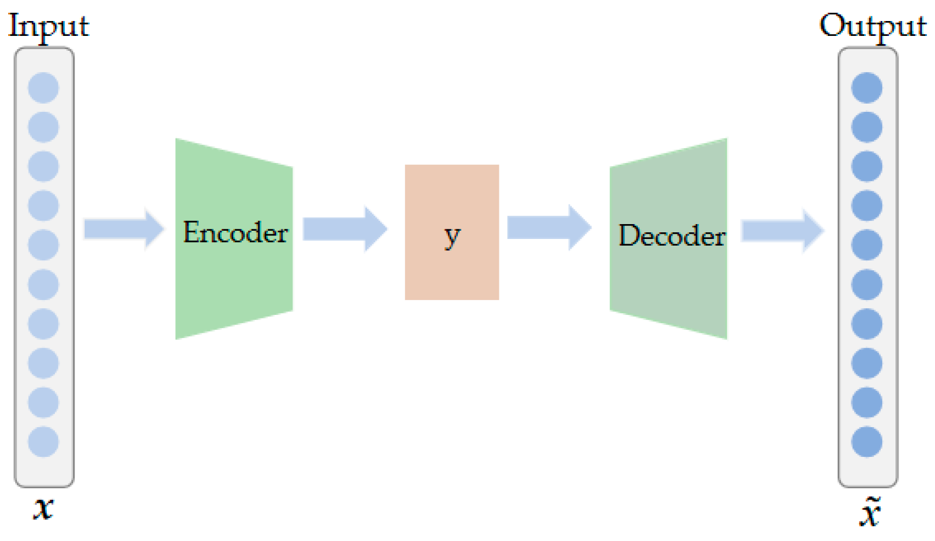
2.1. Autoencoders

As a typical unsupervised deep neural network [21], the AE network is composed of two parts, the encoder and decoder, respectively. The schematic diagram of the network structure is shown in Figure 1.

The encoder maps the input HSI to low-dimensional data, and the decoder reduces it to the original data as much as possible. The parameters of the network include M and b, where M denotes the weight and b denotes the bias. The encoding process from layer x of the input to layer y of the hidden is shown in (1), which represents the encoder correspondence function.

$$y=f\left(x;M,b\right)$$

(1)

The decoding process from hidden layer y to output layer $\tilde{x}$ is shown in (2), $f^{\prime }\left(·\right)$ representing the decoder’s corresponding function, $\tilde{M}$ and $\tilde{b}$ corresponding to M and b, representing the weight and bias of the decoder.

$$\tilde{x}=f^{\prime }\left(y;\tilde{M},\tilde{b}\right)$$

(2)

In the training stage, the reconstruction error is taken as the loss function, and the gradient descent method and back propagation algorithm are used to update the weight and bias parameters until the iteration termination condition is satisfied. The loss function is shown in (3), and L represents the reconstruction error of the whole process.

$$L={‖x-\tilde{x}‖}_2$$

(3)

2.2. Guided Filter

Guided filtering (GF), as an efficient edge filter maintainer [22], has found extensive use in the fields of image fusion [23], feature enhancement [24], and image classification [25] in remote sensing. It is usually able to focus on the image’s specific information and has high efficiency. Its principle is as follows: it assumes that linear transformation is performed on the guide image g in the local window ${\Omega }_j$ centered on pixel j to obtain the output image q, as shown in (4).

$$q_i=a_j{g}_i+b_j,{\forall }_i\in {\Omega }_j$$

(4)

where $\left(2r+1\right)\times (2r+1)$ is the size of the window ${\Omega }_j$. $a_j$ and $b_j$ are linear coefficients calculated by minimizing the difference between the input image p and the output image q within the window, as shown in (5), where the window parameter r and the regularization parameter $\epsilon$ are manual input parameters.

$$E\left(a_j,b_j\right)={\displaystyle \sum _{i\in {\Omega }_j}\left({\left(a_j{g}_i+b_j-p_i\right)}^2+\epsilon a_j^2\right)}$$

(5)

Further, making

$$\begin{array}{c}{\overline{a}}_i={\displaystyle {\sum }_{j\in {\Omega }_i}{a}_j/\left|\Omega \right|}\\ {\overline{b}}_i={\displaystyle {\sum }_{j\in {\Omega }_i}{b}_j/\left|\Omega \right|}\end{array}$$

(6)

where $a_j$ and $b_j$ are, respectively, the average coefficients of sum in all windows ${\Omega }_j$ covering pixel i. Then, the final image $q_i$ after GF is:

$$q_i={\overline{a}}_i{g}_i+{\overline{b}}_i$$

(7)

2.3. Attention Gates

The AG module consists of several functions [26], which are defined as follows:

$${\alpha }_i={\sigma }_2\left({\Psi }^T\left({\sigma }_1\left(W_x^T·x_i+W_g^T·g_i+b_g\right)\right)+b_{\psi }\right)$$

(8)

$${\widehat{x}}_i={\alpha }_i^{}\otimes x_i$$

(9)

where $x_i$ and $g_i$ are the input feature maps; ${\sigma }_1$ and ${\sigma }_2$ are the activation functions of ReLU and Sigmoid, respectively; ${\Psi }^T\in R^{1\times 1}$, $W_x^T\in R^{1\times 1}$, and $W_g^T\in R^{1\times 1}$ are the parameter matrices of the linear transform, which is $1\times 1$ convolution; $b_g\in R^C$ and $b_{\Psi }\in R$ are the bias matrices of the convolution; ${\alpha }_i\in \left[0,1\right]$ is the attention coefficient of the output. The specific model architecture of AG is shown in Figure 2.

Without feature localization, the AG model can automatically respond to the feature region and suppress the response of irrelevant regions at the same time, so that the final output feature map focuses on the region near the mark point.

3. Methodology

This paper proposes the HSI-AD architecture, FCAE-AD, for full convolutional AE with an AG skip connection. The overall framework is shown in Figure 3. It can be divided into two steps. Firstly, the coarse sampling diagram of the encoder and the fine sampling diagram of the decoder are combined to reconstruct the HSI background at the skip connection of the full convolutional AE through the AG. Next, the GF is used to process the initial reconstruction error map to obtain the final detection map. Section 3.1, Section 3.2 and Section 3.3 analyze and discuss the above sections, respectively. To better explain the proposed method, a summary of abbreviations is given in

Table 1. Parameters of different AD algorithms.

Method	Parameters
RX	—
LRX	$wi{n}_{out}=5, wi{n}_{in}=3$
CRD	$\lambda ={10}^{-6}, wi{n}_{out}=11, wi{n}_{in}=3$
GAED	$c=7, l_a=0.4, \beta =1, r_{iter}=300$
Auto-AD	—
MLW_LRRSTO	$W_{L\mathrm{o}cal}=3, \eta =1, \lambda =0.1$
FEBPAD	$p=0.7, r=3, k=0.7\times m\times n$

.

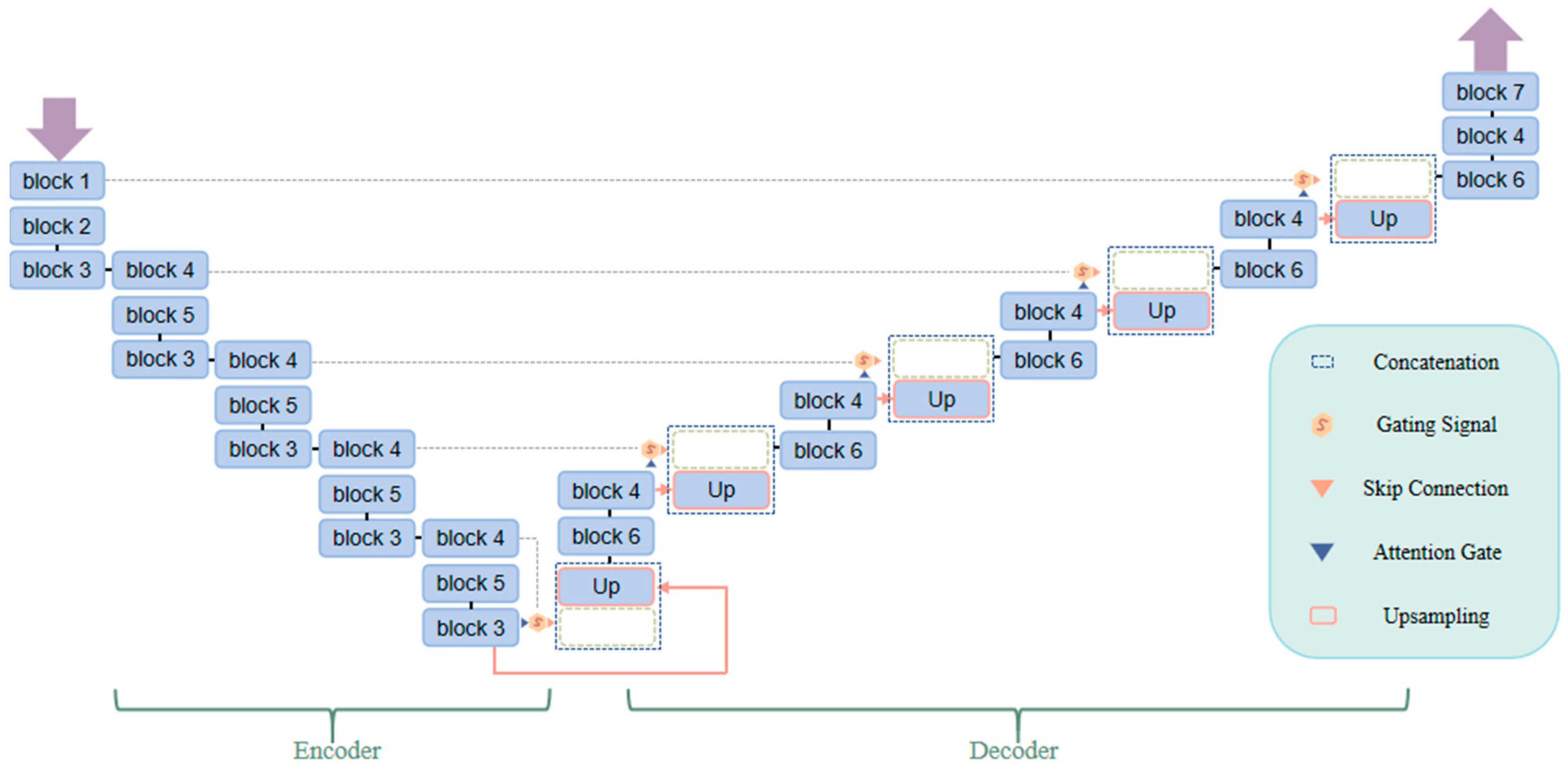
3.1. Full Convolution AE Network Connected by AG

In HSI-AD, HSI can be visually composed of the background and anomaly, and the anomaly can be detected by separating the background. As a result, the precision of anomaly detection is directly impacted by the quality of background separation. To better reconstruct the background, this paper introduces a full convolutional AE network [27], in which the background is obtained by network reconstruction and the reconstruction error is a representation of the anomaly. The grid-based AG module is added to the network’s skip connection to give background pixels more weight to inhibit the reconstruction of anomalies and improve background reconstruction. The proposed AG-connected fully convolutional AE network is shown in Figure 4.

For the HSI ($X\in R^{H\times W\times B}$), where H, W, and B denote the length and width of the X and the number of bands, respectively, the input to the network is a uniform noise distribution of the same size as X, let it be $X_0\in R^{H\times W\times B}$, with a distribution of pixel values in the range $\left[0,1\right]$.

(1)

Encoder: It contains 15 convolutional modules. A convolution layer, a batch normalization (BatchNorm) function, and a leaky rectified linear unit (LeakyReLU) activation function are all included in each convolution module. A $1\times 1$ convolutional layer with a stride of 1 is used in Block 1 and Block 4. Through AG, the created feature maps are linked to the feature maps produced by the respective decoder layers. A $3\times 3$ convolutional layer with a stride of 2 is used in Block 2 and Block 5 primarily for downsampling. In Block 3, to follow Block 2 or Block 5, a $3\times 3$ convolutional layer with a stride of 1 is employed. The feature map dimension is always maintained at 128 dimensions at this stage.

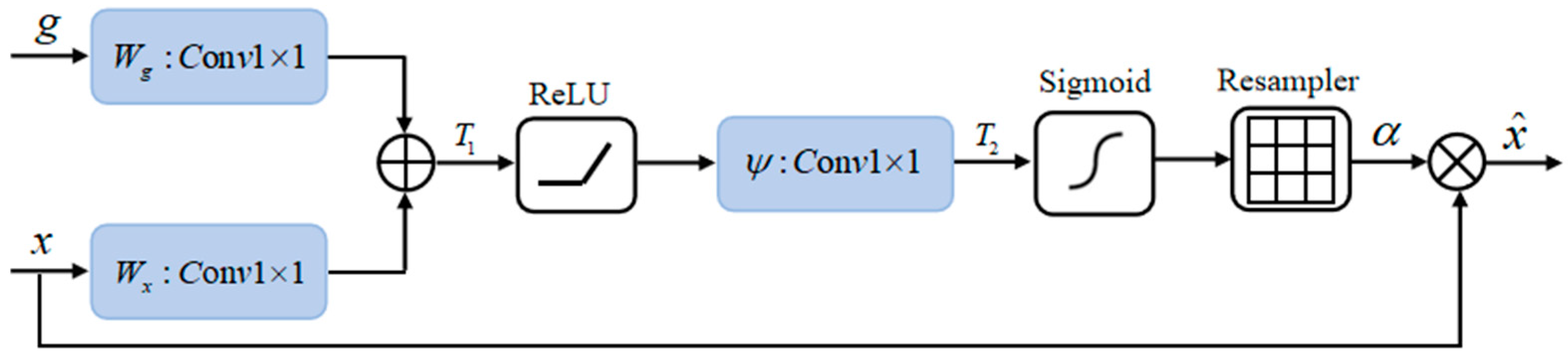
(2)

Converter: It contains 5 AGs with skip connections. The AG model is shown in Figure 1, and its implementation steps are as follows: (a) Convolution is performed on the input feature maps g and x. Then, add the two feature maps to obtain the new feature map. To achieve the purpose of enhancing the feature area; (b) To create the feature map $T_2$, the feature map $T_1$ is first processed by the ReLU activation function and then put through a $1\times 1$ convolution operation; (c) The weight map $\alpha$ (taking values in the range [0, 1]) is obtained after the sigmoid activation function is applied to $T_2$, the background feature area, which tends to 1, and the anomalous feature area, which tends to 0; (d) Resample $\alpha$ and add it to the feature map x to obtain $\stackrel{⌢}{x}$ to enhance the background features and weaken abnormal features [28]. The coarse feature map generated by Block 1 or Block 4 and the fine feature map extracted at multi-scales are sampled, and the complementary information is extracted and fused by AG input before finally being merged into the next Block 6 by skip connection.

(3)

Decoder: It contains 11 convolution modules. Each convolution module has a convolution layer, a BatchNorm layer, and a LeakyReLU layer. The last convolution module also contains a sigmoid activation function. A $3\times 3$ convolution layer with a stride of 1 is used in Block 6, the input is a 256-dimensional feature map that combines the AG feature map with the encoding stage feature map, and the output is a 128-dimensional feature map. Block 4 uses a convolution layer with a step size of 1, following Block 6, with the feature map dimension kept at 128 dimensions. Block 7 uses a convolution layer with a step size of 1 to convert the feature map with a depth of 128 dimensions to the same dimensions as the HSI.

The reconstructed map, with the same size as the original input HSI, is the network’s output.

In the actual training, when the number of training runs increases until it reaches a certain point, the phenomenon of anomalous pixels being reconstructed due to the high fitting of the network will occur. To this end, adaptive weight to the loss function is added to train the model. The reconstruction error is used to construct the weight map, and then the weight map is added to the loss function to construct the weighted loss to train the model [27]. The specific calculation steps are as follows:

$$e_{i,j}={‖x_{i,j}-{\tilde{x}}_{i,j}‖}_2$$

(10)

$$E=\left[e_{1,1},\dots ,e_{1,W};\dots ;e_{H,1},\dots ,e_{H,W}\right]$$

(11)

where, $x_{i,j}$ and ${\tilde{x}}_{i,j}$ represent the pixel vectors of the original image X and the reconstructed image W, respectively. The $e_{i,j}$ represents the reconstruction error between them, and $e_{i,j}$ constitutes the reconstruction error graph E. According to (12), the maximum reconstruction error is subtracted from the value of each reconstruction error to construct the weight graph, and the weighted loss (14) is obtained.

$${\omega }_{i,j}=\max (E)-e_{i,j}$$

(12)

$$Weight=\left[{\omega }_{1,1},\dots ,{\omega }_{1,W};\dots ;{\omega }_{H,1},\dots ,{\omega }_{H,W}\right]$$

(13)

$$L={\displaystyle \sum _{i=1}^H{\displaystyle \sum _{j=1}^W{‖{\omega }_{i,j}\left(x_{i,j}-{\tilde{x}}_{i,j}\right)‖}_2}}$$

(14)

Finally, the loss function is used in the iterative training of the network. The values of the loss function are fed back after each training session to update the network parameters, and the above steps are repeated for each iteration until the average change $\overline{L}$ of the loss function in the last 50 iterations of training is below the threshold $\sigma =1.5\times {10}^{-5}$.

In Algorithm 1, the detailed process of obtaining the reconstructed background image is given by the proposed FCAE-AE network.

Algorithm 1 FCAE-AE network.

Input: HSI $X\in R^{H\times W\times B}$.

Initialization: Random noise map $X_0\in R^{H\times W\times B}$;

Do

1: Network forward;

2: The difference map $\Delta x_i\in E^{H\times W\times B}$ of the X and the network reconstructed background map

Weight is constructed by Formula (11)–(13) for the weight graph;

3: The adaptive weighted loss L is calculated by Formula (14);

4: Network backward;

Until average weighted loss $\overline{L}<\sigma$;

Output: Reconstruct Error E.

3.2. Post Processing Optimization Based on GF

The reconstruction error process usually generates irregular background pixels. To reduce the interference of false anomalies on the detection results, this paper uses GF to process the reconstruction error map E obtained by Section 3.1.

3.2.1. Guide Image Construction

In this paper, we construct the guide image D based on the single-window model [29], using the similarity scores of the image pixel values to be measured with each sub-volume as the pixel values of the guide image. Firstly, the X is divided into 8 sub-volumes, as shown in Figure 5, which can be expressed as $G_j\left(j=1,2,\dots ,8\right)$. The central pixel A is the image pixel to be measured. The difference between each sub-volume $G_j\left(j=1,2,\dots ,8\right)$ and A is calculated separately, as shown in (15).

$$P_j={\displaystyle \sum _{b=1}^B{[A(b)-U_j(b)]}^2}$$

(15)

$A(b)$ denotes the value of the image pixel to be measured in the $bth$ band in X. $U_j$ denotes the average vector of each sub-volume $G_j$ and $U_j(b)$ denotes the value of the $bth$ band of $U_j$. The similarity score $S_j\left(j=1,2,\dots ,8\right)$ between $G_j$ and A is obtained by $P_j$, as shown in (16).

$$S_j=e^{-P_j^2}$$

(16)

$$S_{max}=max(S_j)$$

(17)

The highest score $S_{max}$ in the 8 sub-volumes is selected as the pixel value of guide image D, as shown in (17), where $max\left(·\right)$ denotes the function to select the maximum value.

For this single-window model, there may be four possible cases, as follows:

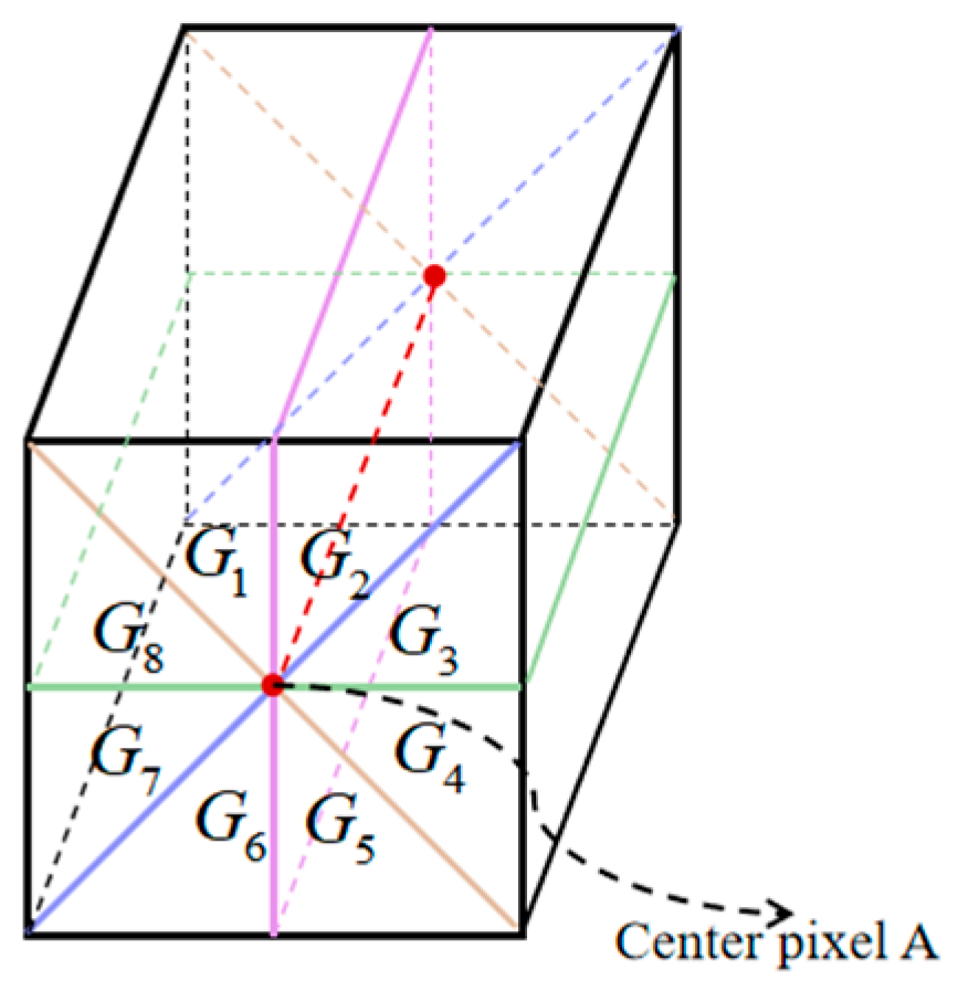
(a)

Both the pixel to be measured and the window pixels are the background. The similarity scores $S_j$ of the image pixel A to be measured and all sub-volumes $G_j\left(j=1,2,\dots ,8\right)$ are high.

(b)

The pixel to be measured is the background, but there are anomalies in the window. The similarity scores $S_j$ between $G_j$ containing the anomaly and the image pixel A to be tested are lower than those of $G_j$ not containing the anomalous pixels.

(c)

The image pixel to be measured is anomalous, but the pixels in the window are background. All values are very low, and it is easy to determine that the image element A to be measured is anomalous.

(d)

The image pixel to be measured is anomalous, and window pixels also have anomalous pixels. The similarity score $S_j$ between $G_j$ containing anomalies and pixel A to be measured is higher than $G_j$ without anomalies. However, in the actual HSI, anomalies only occupy a few, so the situation almost does not exist.

3.2.2. Process of Guide Filtering

The reconstruction error map E is taken as the input image of GF, and we can get the final detection map under the correction of the above guide image D. The specific process is shown in (18), and the process figure is shown in Figure 6.

$$F_i={\overline{a}}_i·\Delta x_i+{\overline{b}}_i,F_i\in F_{final},\Delta x_i\in E$$

(18)

where ${\overline{a}}_i$ and ${\overline{b}}_i$ represent the average of the linear function coefficients $\left(a_i,b_i\right)$ covering all overlapping windows of $\Delta x_i$, respectively. See (6) for the calculation function.

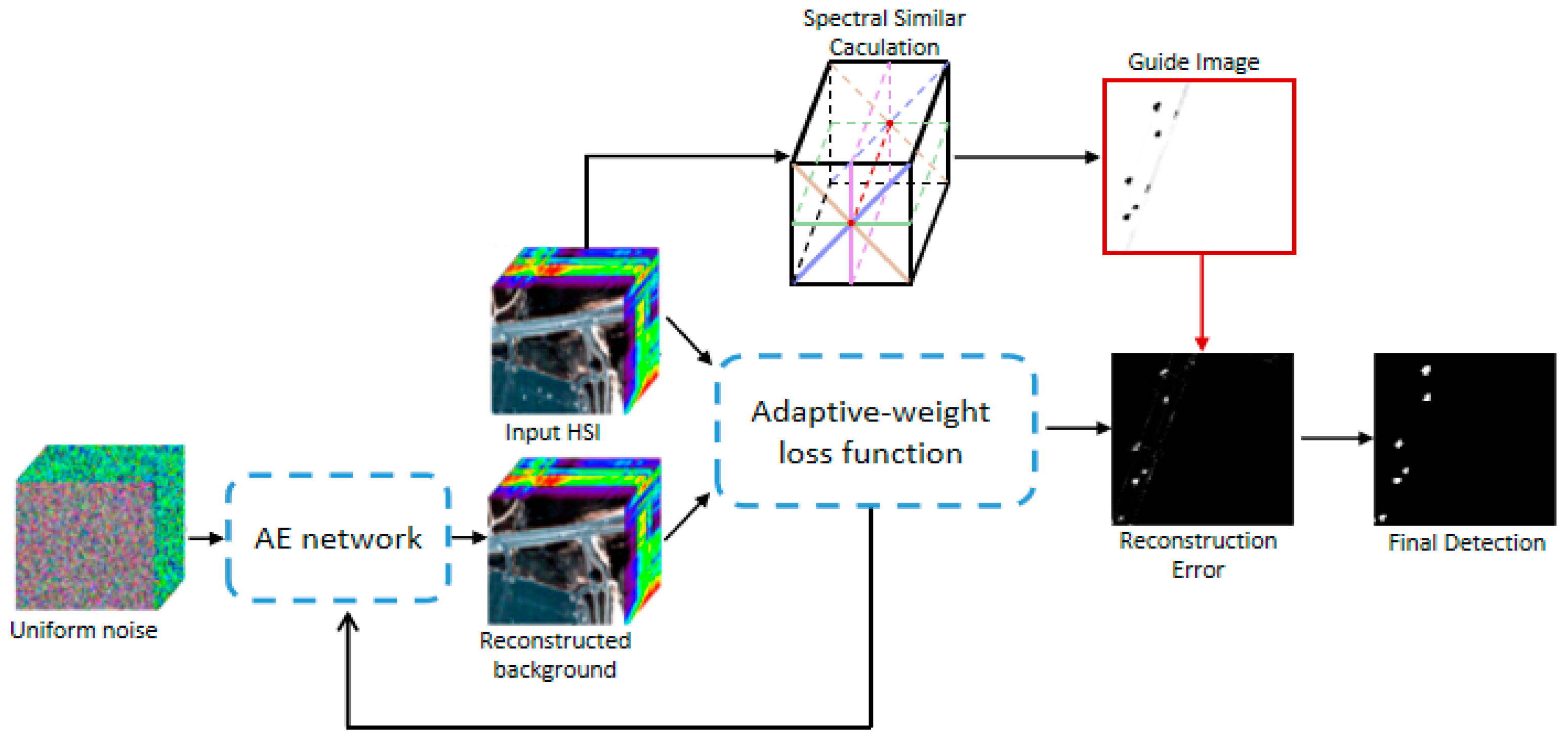
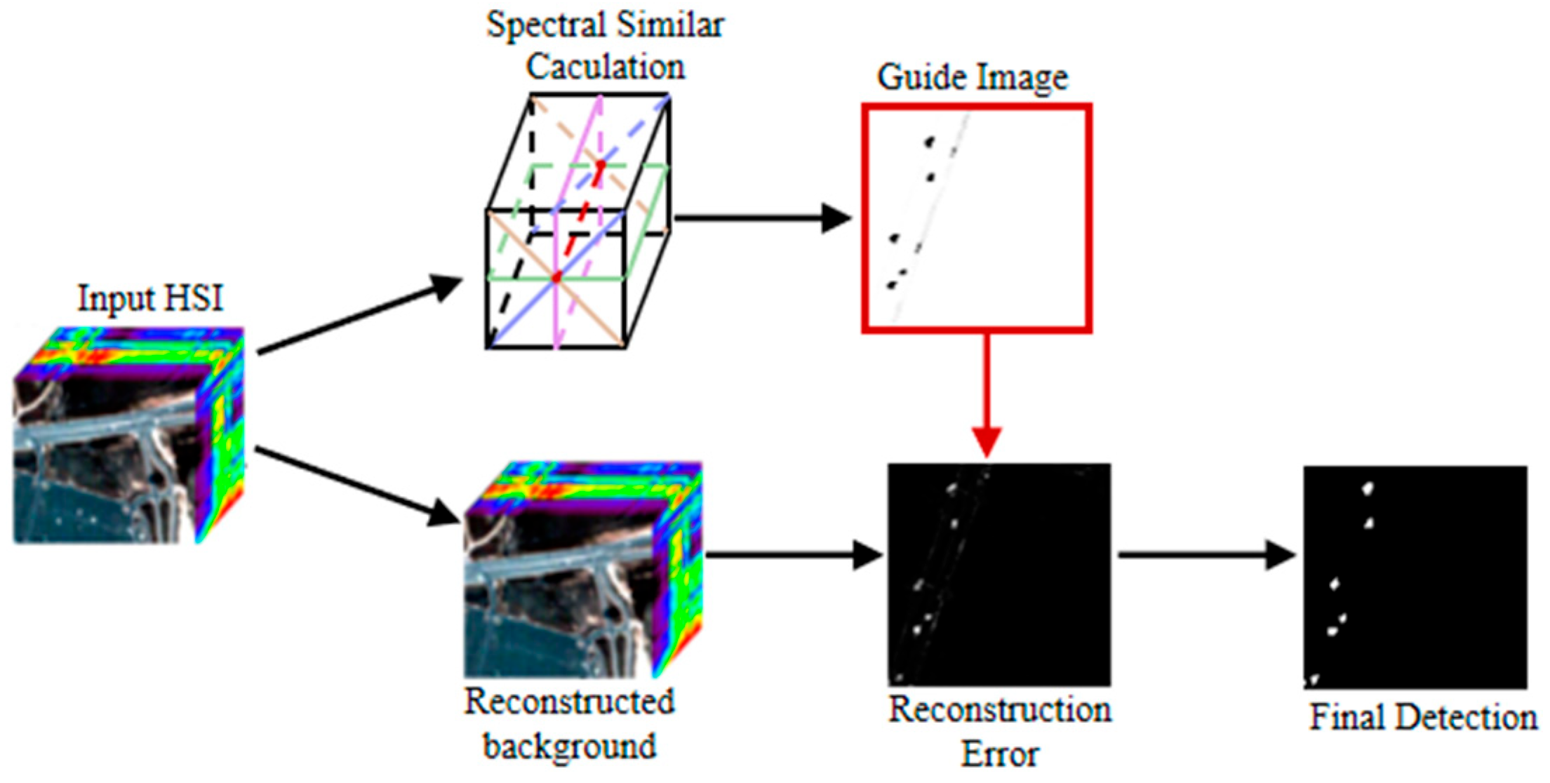
3.3. Algorithm Implementation

Based on the above analysis, a fully convolutional HSI-AD algorithm with AG connection is proposed, and the method steps are given in Algorithm 2.

Algorithm 2 Overall framework.

Input: HSI $X\in R^{H\times W\times B}$.

Initialization: Random noise map $X_0\in R^{H\times W\times B}$; Window size c; Guide filter size r; Guide filter

regularization parameters $\epsilon$.

1: The random noise $X_0$ image is input into the network, and the background reconstruction

image W is obtained by Algorithm 1 after the correction of the X;

2: The reconstruction error E is obtained by the X and the W;

3: The X is divided into 8 volumes by the single-window model, and the difference $P_j$

between each sub-volume $G_j$ and the pixel A to be measured is calculated by Formula (15);

4: The similarity score $S_j$ of $G_j$ and A is calculated by Formula (16);

5: According to Formula (17), the highest score $S_{\max }$ in $S_j(j=1,2,\dots ,8)$ is selected as the pixel

value to guide image D;

6: The final detection image $F_{final}$ is obtained by GF the residual map E with the guide image D;

Output: Anomaly Detection Map $F_{final}$.

4. Analysis and Experiment

In this paper, the experimental environment is the Windows 10 operating system, the experimental computer configuration is an Intel Core i7-7700 CPU and 16 GB RAM, and the experimental platform is Python 3.7.

4.1. Experimental Datasets

The four real public datasets are adopted, which are, respectively, the Gulfport Airport, Texas Coast, Cat Island, and HYDICE Urban datasets [30]. The details are as follows:

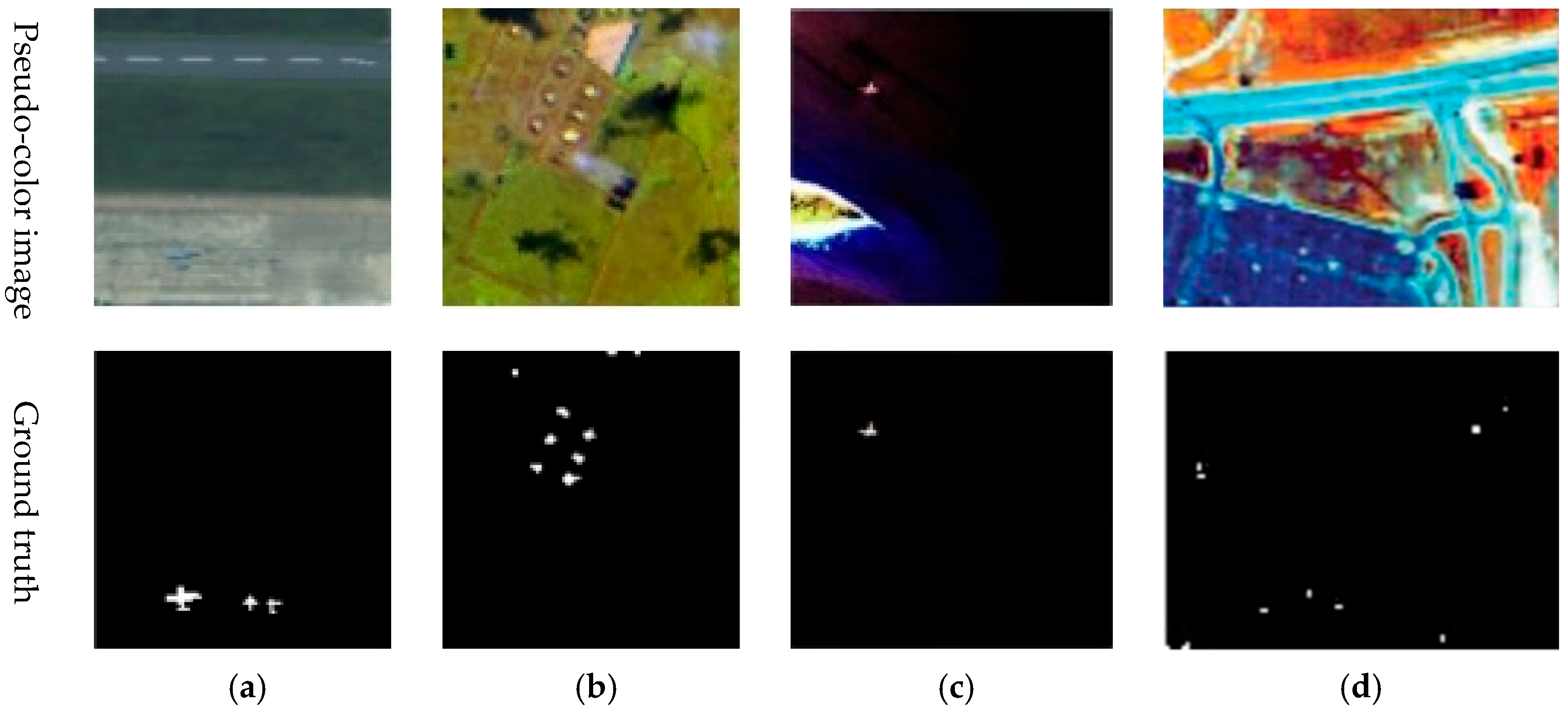
(1)

Gulfport Airport: The dataset has a spatial resolution of 3.5 m and was acquired by the AVIRIS sensor in Gulfport, Mississippi, in the United States. The size is 100 × 100 and the total number of spectral bands is 191 spectral bands. The anomalous area that must be found is the aircraft in the photograph. The sample image and the ground truth map for this dataset are displayed in Figure 7a.

(2)

Texas Coast: The dataset, which has a size of 100 × 100, a spatial resolution of 17.2 m, and 204 bands, was acquired by AVIRIS sensors off the Texas coast. Residents’ houses of various shapes in the image are marked as anomaly, containing 155 anomalous pixels. The sample image and the ground truth map for this dataset are displayed in Figure 7b.

(3)

Cat Island: The dataset was acquired by the AVIRIS sensor over the beaches and sea areas surrounding Cat Island and contains 188 spectral bands in an image of size 150 × 150. The dataset includes 19 anomalous pixels from airplane scenes. The sample image and the ground truth map for this dataset are displayed in Figure 7c.

(4)

HYDICE Urban: The dataset was acquired by the HYDICE sensor in an urban area in California, USA. The size of the test image used in the experiment is 80 × 100. After removing the noise band, there are still 175 spectral bands remaining. and the spatial resolution is 3 m. It contains 17 anomalous pixels, including cars and roofs. The example image and ground truth map for this dataset are shown in Figure 7d.

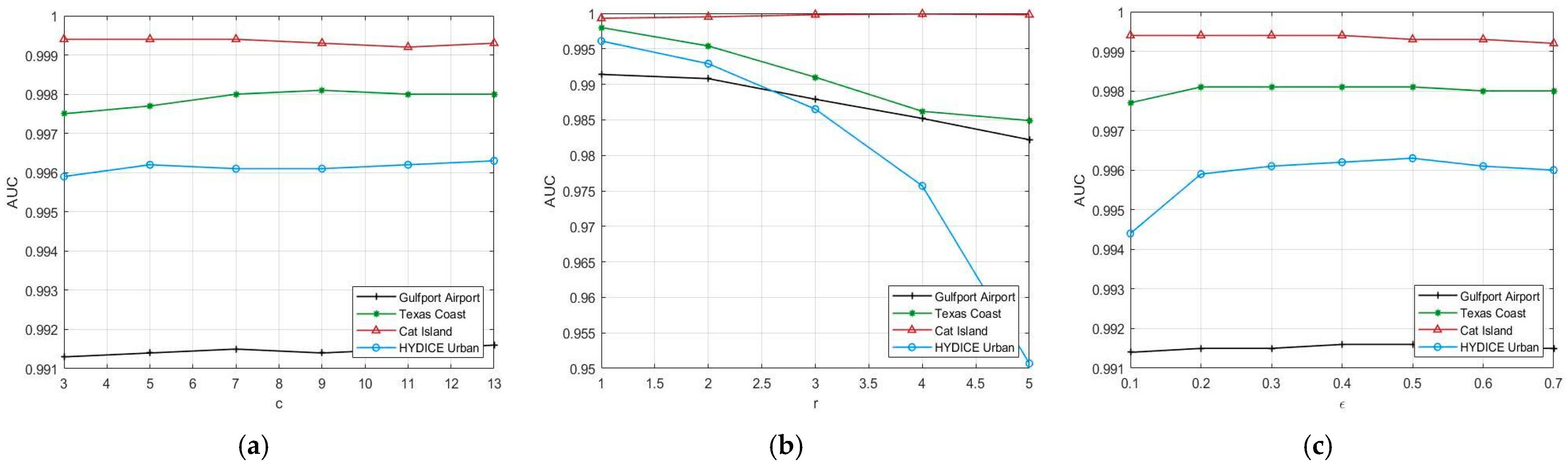
4.2. Parameter Setting

Several classical AD algorithms are selected for comparison experiments in this paper, including the RX algorithm [3], the LRX algorithm [4], the Auto-AD algorithm [27], the guided autoencoder algorithm (GAED) [29], the Low-Rank Representation incorporating a spatial constraint (MLW_LRRSTO) algorithm [31], and the feature extraction and background purification for anomaly detection (FEBPAD) algorithm [32], the CRD algorithm [33].

To get the best detection result possible from each algorithm, parameters are set in each algorithm. Table 1 shows the parameter settings of the relevant algorithms.

The FCAE-AD algorithm in this paper contains three parameters, which are window size c, guided filtering size r, and regularization parameter $\epsilon$. The effects of different parameter settings on FCAE-AD results are evaluated based on the AUC using the four common datasets mentioned above.

To analyze a particular parameter, the other parameters are left unchanged, and the default value is set to c = 9, r = 1, $\epsilon =0.5$. The AUC line graphs concerning the parameter variation are shown in Figure 8.

(1)

Window size c: A line chart of the AUC values with parameter c is shown in Figure 8a. The AUC value of Gulfport Airport fluctuates up and down in the general trend and reaches its peak when c = 13, so the Gulfport Airport window size c is set to 13. For Texas Coast, the general trend of AUC value is increasing first, then decreasing to reach the peak at c = 9. Therefore, the Texas Coast window size c is set to 9. For Cat Island, the AUC value is constant from window sizes 3–9 and decreasing from c = 9, so the Cat Island window size c is set to 9. For HYDICE Urban, the AUC value tends to increase all the time, so the HYDICE Urban window size c is set to 13. To sum up, the parameters c for the above four datasets are set to 13, 9, 9, and 13, respectively. In the order given in Section 4.1.

(2)

Guide filter size r: A line chart of the AUC values with parameter r is shown in Figure 8b. The general trend of the AUC value for Cat Island increases from r = 1 to decreases at r = 4. For Gulfport Airport, Texas Coast, and HYDICE Urban, the AUC value decreases from r = 1. To sum up, r of Cat Island is set to 4 in this paper, and r of other datasets is set to 1.

(3)

Guide filter regularization parameters $\epsilon$: A line chart of the AUC values with parameter $\epsilon$ is shown in Figure 8c. As we can see from the figure, for Gulfport Airport and HYDICE Urban, the general trend of the AUC value decreases from $\epsilon =0.1$ to $\epsilon =0.5$, so the above two datasets $\epsilon$ are 0.5. For Texas Coast, the general trend of the AUC value is to first increase to $\epsilon =0.2$, stabilize to $\epsilon =0.5$, and then decrease, so the value of $\epsilon$ for Texas Coast is 0.2. For Cat Island, the AUC value first stays the same at $\epsilon =0.4$ and then decreases, so $\epsilon$ for Cat Island is 0.4. To sum up, parameter $\epsilon$ is set to 0.5, 0.2, 0.4, and 0.5, respectively, in the sequence of datasets in Section 4.1.

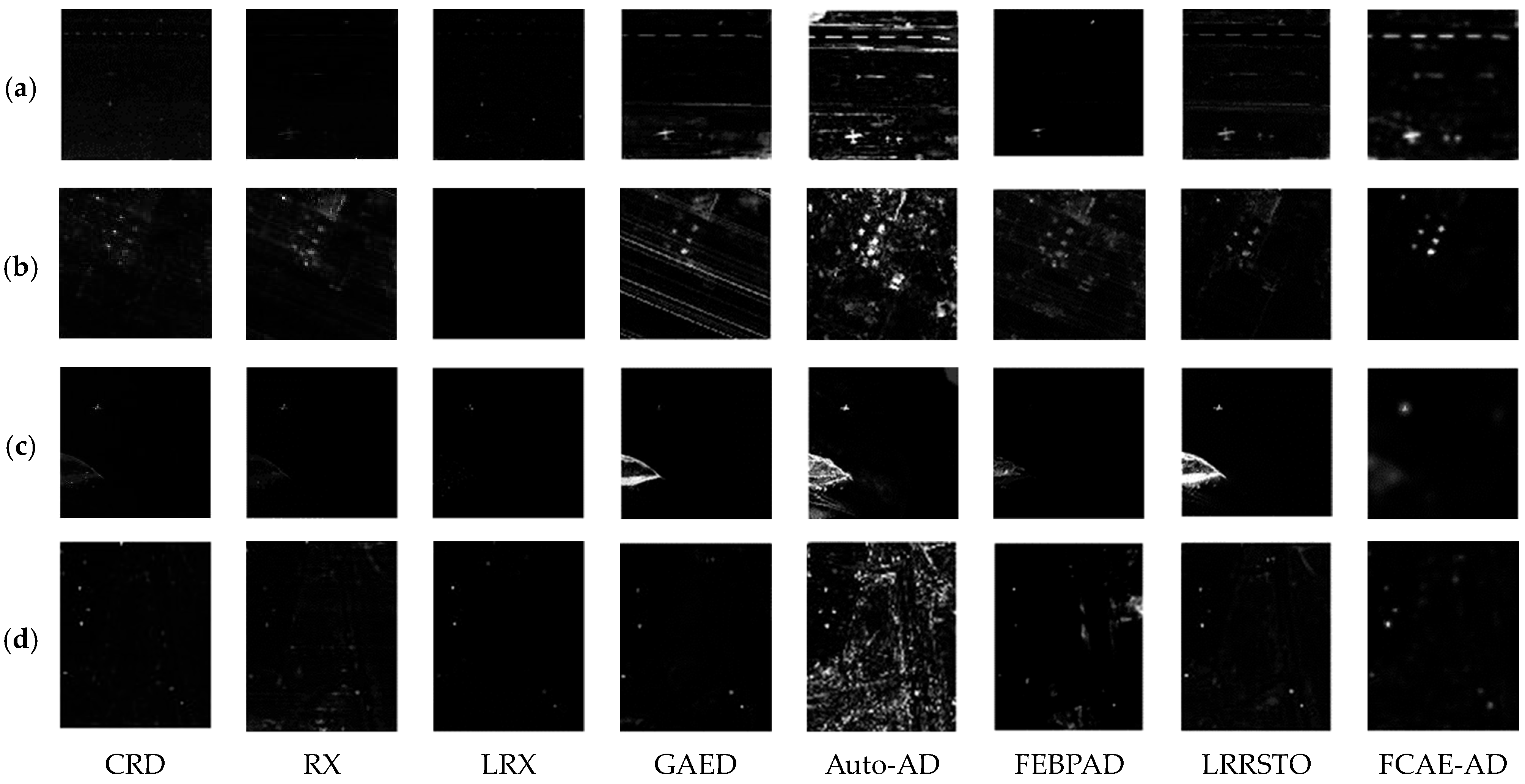
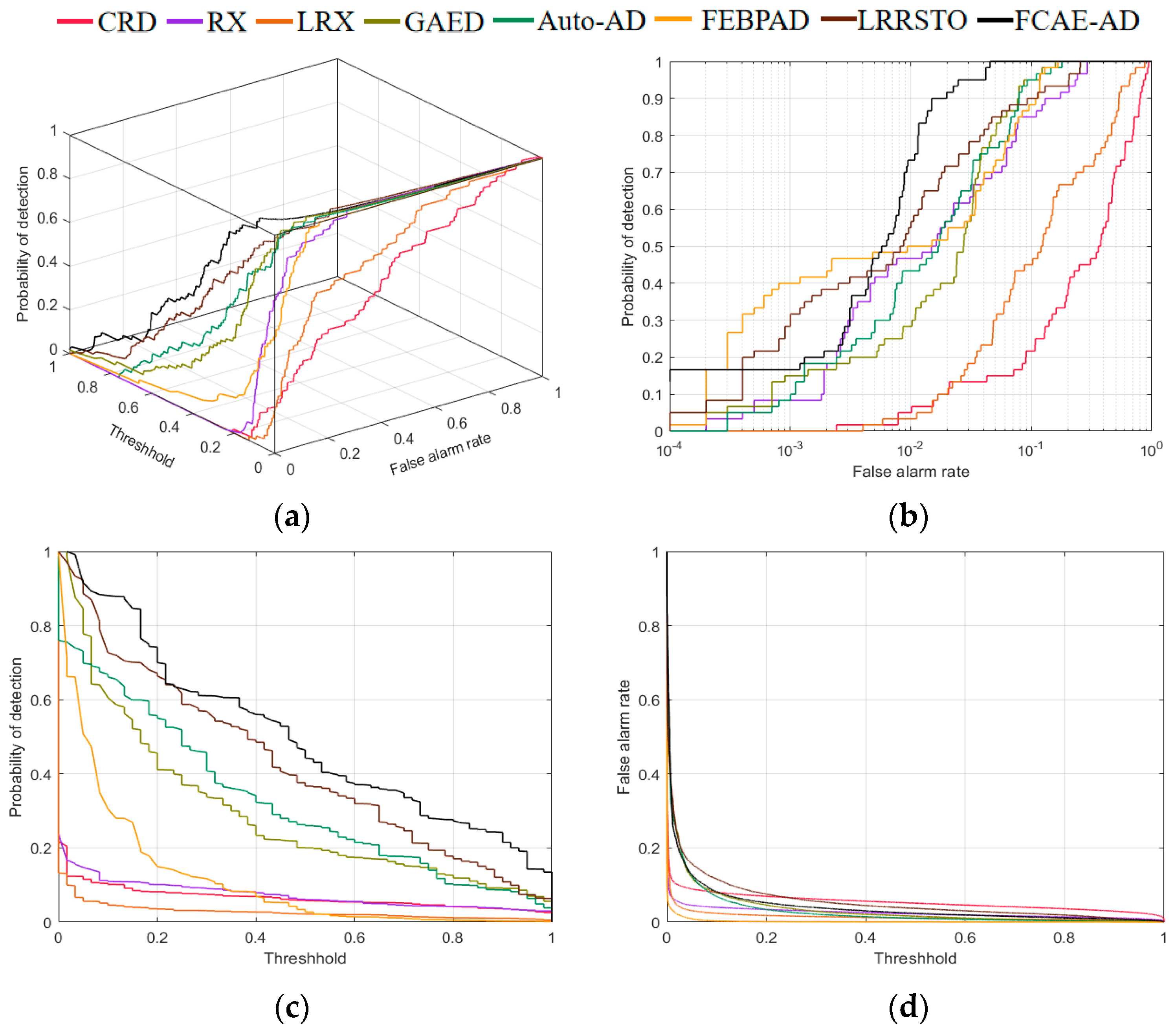
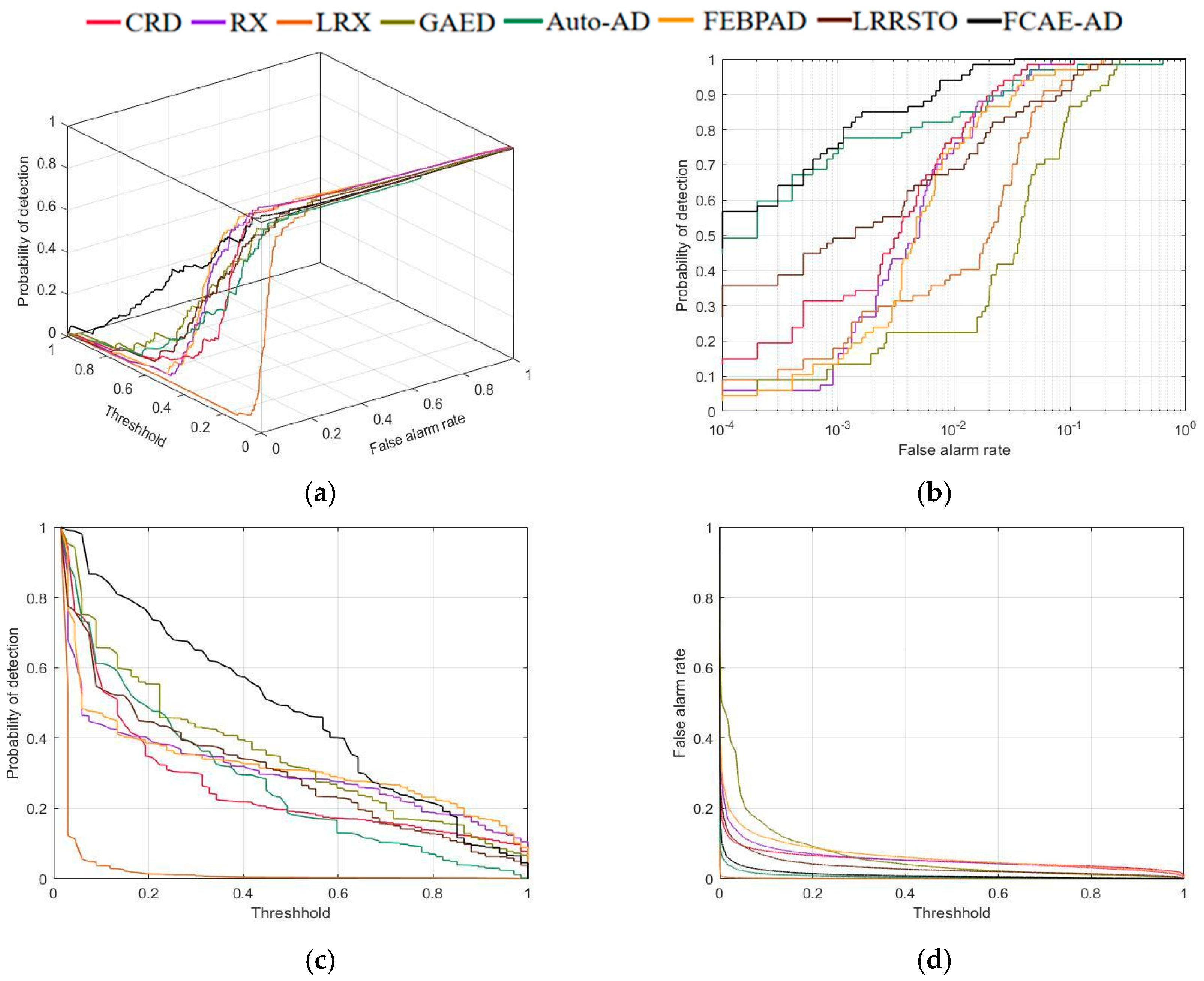
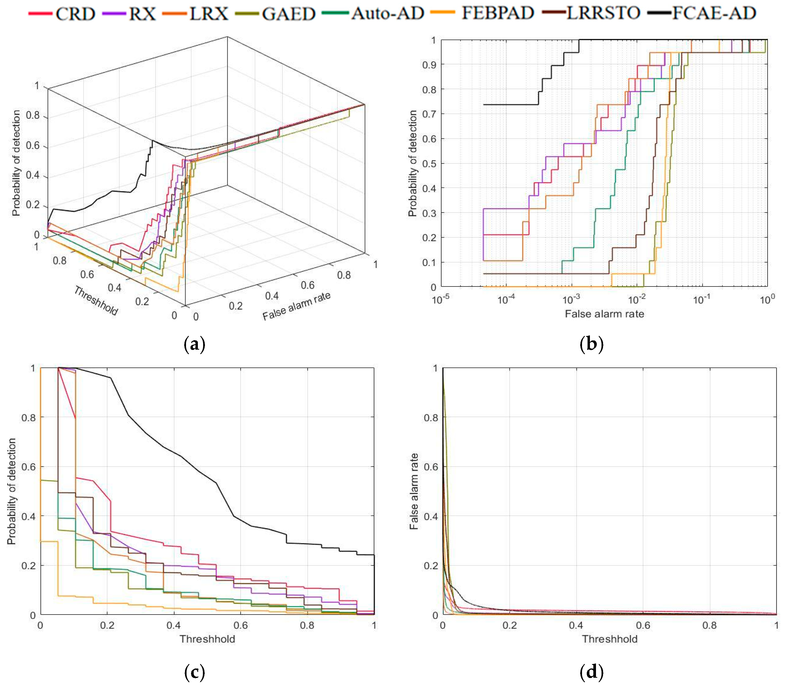
4.3. Analysis and Comparison of Detection Results

In order to analyze the detection results effectively, this paper adopts the corresponding three-dimensional receiver operating characteristic (3-D ROC) curve, the corresponding two-dimensional ROC (2-D ROC) curve $\left(P_D,P_F\right)$, 2-D ROC curve $\left(P_D,\tau \right)$, 2-D ROC curve $\left(P_F,\tau \right)$ [34], and some evaluation indicators $AU{C}_{TD}$, $AU{C}_{BS}$, $AU{C}_{SNPR}$, $AU{C}_{TDBS}$, $AU{C}_{OTD}$ for quantitative analysis. Where $AU{C}_{TD}$, $AU{C}_{BS}$, $AU{C}_{SNPR}$, $AU{C}_{TDBS}$, $AU{C}_{OTD}$ are generated by calculating $\left(P_D,P_F\right)$, $\left(P_D,\tau \right)$, $\left(P_F,\tau \right)$, respectively. They are calculated as follows:

$$\left\{\begin{array}{c}\begin{array}{c}AU{C}_{TD}=AU{C}_{\left(D,F\right)}+AU{C}_{\left(D,\tau \right)}\\ AU{C}_{BS}=AU{C}_{\left(D,F\right)}-AU{C}_{\left(F,\tau \right)}\end{array}\\ AU{C}_{SNPR}=\frac{AU{C}_{\left(D,\tau \right)}}{AU{C}_{\left(F,\tau \right)}}\\ \begin{array}{c}AU{C}_{TDBS}=AU{C}_{\left(D,\tau \right)}-AU{C}_{\left(F,\tau \right)}\\ AU{C}_{ODP}=AU{C}_{\left(D,F\right)}+AU{C}_{\left(D,\tau \right)}-AU{C}_{\left(F,\tau \right)}.\end{array}\end{array}\right.$$

where $AU{C}_{\left(D,F\right)}$, $AU{C}_{TDBS}$, and $AU{C}_{OTD}$ represent the overall performance. $AU{C}_{\left(D,\tau \right)}$, $AU{C}_{TD}$, and $AU{C}_{\left(F,\tau \right)}$ represent the target detection rate. $AU{C}_{BS}$ and $AU{C}_{SNPR}$ represent the background suppression rate. The better, the smaller the value of $AU{C}_{\left(F,\tau \right)}$. The better, the larger the remaining value [29].

To analyze the detection performance of the FCAE-AD algorithm proposed in this paper, the detection result graphs of different algorithms are compared, and the detection results of each algorithm on different datasets are shown in Figure 9. It can be seen from the figure that although the CRD algorithm, RX algorithm, LRX algorithm, and FCBPAD algorithm have good background suppression effects, they cannot realize the separation of anomaly and background in most cases. Although the Auto-AD algorithm can detect the anomaly, the background suppression effect is not good enough overall. The detection results of the GAED algorithm and the LRRSTO algorithm are close to the FCAE-AD algorithm, but the background of the GAED algorithm in the second dataset is relatively clear, and the anomaly separation effect of the LRRSTO algorithm is not as good as that of the FCAE-AD algorithm. From the point of view of subjective analysis, the FCAE-AD algorithm proposed in this paper has achieved relatively good results on various datasets.

For the Gulfport Airport experimental dataset, the FCAE-AD algorithm achieves very significant results. The data given in

Table 2. Comparison of AUC performance of Gulfport Airport on different algorithms.

Method	$\mathit{A}\mathit{U}{\mathit{C}}_{(\mathit{D},\mathit{F})}\uparrow$	$\mathit{A}\mathit{U}{\mathit{C}}_{(\mathit{D},\mathit{\tau })}\uparrow$	$\mathit{A}\mathit{U}{\mathit{C}}_{(\mathit{F},\mathit{\tau })}\downarrow$	$\mathit{A}\mathit{U}{\mathit{C}}_{\mathit{T}\mathit{D}}\uparrow$	$\mathit{A}\mathit{U}{\mathit{C}}_{\mathit{B}\mathit{S}}\uparrow$	$\mathit{A}\mathit{U}{\mathit{C}}_{\mathit{S}\mathit{N}\mathit{P}\mathit{R}}\uparrow$	$\mathit{A}\mathit{U}{\mathit{C}}_{\mathit{T}\mathit{D}\mathit{B}\mathit{S}}\uparrow$	$\mathit{A}\mathit{U}{\mathit{C}}_{\mathit{O}\mathit{D}\mathit{P}}\uparrow$
CRD	0.6272	0.0660	0.0541	0.6932	0.5731	1.2208	0.0119	0.6391
RX	0.9526	0.0736	0.0248	1.0262	0.9278	2.9743	0.0489	1.0015
LRX	0.7917	0.0277	0.0144	0.8194	0.7773	1.9235	0.0133	0.8050
GAED	0.9680	0.2930	0.0347	1.2609	0.9333	8.4396	0.2582	1.2262
Auto-AD	0.9696	0.3230	0.0302	1.2926	0.9394	10.6847	0.2928	1.2624
FEBPAD	0.9664	0.1116	0.0023	1.0779	0.9641	48.9449	0.1093	1.0756
LRRSTO	0.9687	0.4239	0.0552	1.3926	0.9135	7.6839	0.3687	1.3374
FCAE-AD	0.9916	0.5013	0.0416	1.4929	0.9500	12.0475	0.4597	1.4513

shows that most of the $AU{C}_{(D,F)}$ scores of the other comparison algorithms are around or below 0.96, while the AUC score of the FCAE-AD algorithm is above 0.99. In addition, the $AU{C}_{(D,\tau )}$, $AU{C}_{TD}$, $AU{C}_{BS}$, $AU{C}_{SNPR}$, $AU{C}_{TDBS}$ and $AU{C}_{ODP}$ values of the FCAE-AD algorithm are much larger than those of the other compared algorithms. The best values are shown in bold. Although the performance of the FCAE-AD algorithm on $AU{C}_{(F,\tau )}$ is not the best, it has achieved certain competitive results. As shown in Figure 10, the 3D-ROC curve and the corresponding 2D-ROC curves $\left(P_D,P_F\right)$ and $\left(P_D,\tau \right)$ of the proposed algorithm are both higher than other comparison algorithms, and the 2D-ROC curve $\left(P_F,\tau \right)$ also achieves relatively good results. In particular, according to Figure 10b, it can be seen from the image that when $P_D$ reaches 100%, the $P_F$ of FCAE-AD algorithm is also lower than others, the algorithm proposed in this paper has a lower false positive rate than others, which indicates that the anomaly and background are well separated. In conclusion, FCAE-AD has advantages in most indexes.

According to Figure 11, the 3D-ROC curve, the 2D-ROC curves $\left(P_D,P_F\right)$ and $\left(P_D,\tau \right)$ of the FCAE-AD algorithm are significantly greater than those of the other compared algorithms. The 2D-ROC curve of $\left(P_F,\tau \right)$ is shown in Figure 11d, and relatively good results are also obtained. It is seen from

Table 3. Comparison of AUC performance of Texas Coast on different algorithms.

Method	$\mathit{A}\mathit{U}{\mathit{C}}_{(\mathit{D},\mathit{F})}\uparrow$	$\mathit{A}\mathit{U}{\mathit{C}}_{(\mathit{D},\mathit{\tau })}\uparrow$	$\mathit{A}\mathit{U}{\mathit{C}}_{(\mathit{F},\mathit{\tau })}\downarrow$	$\mathit{A}\mathit{U}{\mathit{C}}_{\mathit{T}\mathit{D}}\uparrow$	$\mathit{A}\mathit{U}{\mathit{C}}_{\mathit{B}\mathit{S}}\uparrow$	$\mathit{A}\mathit{U}{\mathit{C}}_{\mathit{S}\mathit{N}\mathit{P}\mathit{R}}\uparrow$	$\mathit{A}\mathit{U}{\mathit{C}}_{\mathit{T}\mathit{D}\mathit{B}\mathit{S}}\uparrow$	$\mathit{A}\mathit{U}{\mathit{C}}_{\mathit{O}\mathit{D}\mathit{P}}\uparrow$
CRD	0.9918	0.2739	0.0527	1.2657	0.9390	5.1932	0.2212	1.2129
RX	0.9907	0.3143	0.0556	1.3049	0.9351	5.6570	0.2587	1.2494
LRX	0.9711	0.0372	0.0008	1.0083	0.9703	44.4876	0.0363	1.0075
GAED	0.9436	0.3644	0.0631	1.3080	0.8805	5.7757	0.3013	1.2449
Auto-AD	0.9846	0.2840	0.0060	1.2686	0.9786	47.0579	0.2779	1.2626
FEBPAD	0.9861	0.3297	0.0648	1.3158	0.9213	5.0863	0.2649	1.2510
LRRSTO	0.9802	0.3122	0.0326	1.2924	0.9476	9.5783	0.2796	1.2598
FCAE-AD	0.9981	0.4808	0.0108	1.4789	0.9873	44.5410	0.4700	1.4681

that the maximum $AU{C}_{(D,F)}$ score of the algorithm in this paper is 0.9981. In addition, the $AU{C}_{(D,\tau )}$, $AU{C}_{TD}$, $AU{C}_{BS}$, $AU{C}_{TDBS}$, and $AU{C}_{ODP}$ values of the FCAE-AD algorithm are much higher than those of other comparison algorithms. The best values are shown in bold. Although the performance of the FCAE-AD algorithm on $AU{C}_{(F,\tau )}$ is not the best, it has achieved certain competitive results. Although the result of $AU{C}_{SNPR}$ is not optimal, it is second only to the Auto-AD algorithm. Combined with these results, FCAE-AD has the advantage in most indexes.

The 3D-ROC curve, 2D-ROC curves, and corresponding AUC values of several algorithms in the Cat Island experimental dataset are displayed in Figure 12 and

Table 4. Comparison of AUC performance of Cat Island on different algorithms.

Method	$\mathit{A}\mathit{U}{\mathit{C}}_{(\mathit{D},\mathit{F})}\uparrow$	$\mathit{A}\mathit{U}{\mathit{C}}_{(\mathit{D},\mathit{\tau })}\uparrow$	$\mathit{A}\mathit{U}{\mathit{C}}_{(\mathit{F},\mathit{\tau })}\downarrow$	$\mathit{A}\mathit{U}{\mathit{C}}_{\mathit{T}\mathit{D}}\uparrow$	$\mathit{A}\mathit{U}{\mathit{C}}_{\mathit{B}\mathit{S}}\uparrow$	$\mathit{A}\mathit{U}{\mathit{C}}_{\mathit{S}\mathit{N}\mathit{P}\mathit{R}}\uparrow$	$\mathit{A}\mathit{U}{\mathit{C}}_{\mathit{T}\mathit{D}\mathit{B}\mathit{S}}\uparrow$	$\mathit{A}\mathit{U}{\mathit{C}}_{\mathit{O}\mathit{D}\mathit{P}}\uparrow$
CRD	0.9685	0.2935	0.0184	1.2620	0.9501	15.9346	0.2751	1.2435
RX	0.9807	0.2496	0.0065	1.2304	0.9742	38.1909	0.2431	1.2238
LRX	0.9934	0.1933	0.0011	1.1867	0.9923	177.5045	0.1923	1.1856
GAED	0.9223	0.1100	0.0172	1.0323	0.9050	6.3794	0.0928	1.0151
Auto-AD	0.9640	0.1509	0.0026	1.1149	0.9613	57.1912	0.1483	1.1122
FEBPAD	0.9663	0.0404	0.0046	1.0067	0.9616	8.7300	0.0358	1.0020
LRRSTO	0.9596	0.2198	0.0104	1.1794	0.9492	21.1154	0.2094	1.1690
FCAE-AD	0.9998	0.5799	0.0168	1.5749	0.9830	34.5258	0.5631	1.5629

, respectively. As demonstrated by the figure, when compared to other algorithms, the FCAE-AD curve is substantially higher. According to Figure 12b, the 2D-ROC curve $\left(P_D,P_F\right)$ of the AG-AD algorithm is significantly greater than that of the other compared algorithms. According to the image, when $P_D$ reaches 100%, the $P_F$ value of the FCAE-AD algorithm is much lower than others, so the false positive rate of the algorithm in this paper is lower than others, which indicates that the anomaly and background are well separated. As demonstrated by the table, the $AU{C}_{(D,F)}$ score of the algorithm in this paper is 0.9998, which is very near 1. In addition, the values of $AU{C}_{(D,\tau )}$, $AU{C}_{TD}$, $AU{C}_{TDBS}$ and $AU{C}_{ODP}$ of FCAE-AD algorithm are much higher than those of other comparison algorithms. The best values are shown in bold. Although the performance of the FCAE-AD algorithm on $AU{C}_{(F,\tau )}$, $AU{C}_{BS}$ and $AU{C}_{SNPR}$ is not the best, it still achieves certain competitive results. Although the result of $AU{C}_{SNPR}$ is not optimal, it is second only to the Auto-AD algorithm. Combined with these results, FCAE-AD has the advantage in most indexes.

The 3D-ROC curve, 2D-ROC curves, and corresponding AUC values of several algorithms in the HYDICE Urban experimental dataset are displayed in Figure 13 and

Table 5. Comparison of AUC performance of HYDICE Urban on different algorithms.

Method	$\mathit{A}\mathit{U}{\mathit{C}}_{(\mathit{D},\mathit{F})}\uparrow$	$\mathit{A}\mathit{U}{\mathit{C}}_{(\mathit{D},\mathit{\tau })}\uparrow$	$\mathit{A}\mathit{U}{\mathit{C}}_{(\mathit{F},\mathit{\tau })}\downarrow$	$\mathit{A}\mathit{U}{\mathit{C}}_{\mathit{T}\mathit{D}}\uparrow$	$\mathit{A}\mathit{U}{\mathit{C}}_{\mathit{B}\mathit{S}}\uparrow$	$\mathit{A}\mathit{U}{\mathit{C}}_{\mathit{S}\mathit{N}\mathit{P}\mathit{R}}\uparrow$	$\mathit{A}\mathit{U}{\mathit{C}}_{\mathit{T}\mathit{D}\mathit{B}\mathit{S}}\uparrow$	$\mathit{A}\mathit{U}{\mathit{C}}_{\mathit{O}\mathit{D}\mathit{P}}\uparrow$
CRD	0.9943	0.3212	0.0288	1.3155	0.9655	11.1567	0.2924	1.2867
RX	0.9857	0.2404	0.0351	1.2261	0.9506	6.8442	0.2053	1.1910
LRX	0.9922	0.2217	0.0039	1.2139	0.9883	56.8040	0.2178	1.2100
GAED	0.9649	0.3409	0.0082	1.3058	0.9567	41.6638	0.3327	1.2976
Auto-AD	0.9790	0.3100	0.0085	1.2889	0.9705	36.6122	0.3015	1.2805
FEBPAD	0.9357	0.1561	0.0130	1.0919	0.9227	11.9830	0.1431	1.0788
LRRSTO	0.9953	0.4769	0.0346	1.4722	0.9607	13.7852	0.4423	1.4376
FCAE-AD	0.9963	0.3018	0.0202	1.2981	0.9760	14.9082	0.2816	1.2778

, respectively. As demonstrated by Figure 13a,b, the 3D-ROC curve and the 2D-ROC curve $\left(P_D,P_F\right)$ of the FCAE-AD algorithm are superior to other comparison algorithms. The 2D-ROC curves of $\left(P_D,\tau \right)$ and $\left(P_F,\tau \right)$ are shown in Figure 13c,d. As can be seen from the table, the $AU{C}_{(D,\tau )}$ value in this paper is the highest, 0.9963. The best values are shown in bold. Although the values of other $AU{C}_{(D,\tau )}$, $AU{C}_{TD}$, $AU{C}_{TDBS}$, $AU{C}_{ODP}$, $AU{C}_{(F,\tau )}$, $AU{C}_{BS}$, and $AU{C}_{SNPR}$ indexes in this paper are not optimal, some competitive results have been obtained.

4.4. Ablation Study

To further explore the effectiveness of the proposed algorithm, detailed ablation experiments of the FCAE-AD algorithm are conducted in this section.

The FCAE-AD algorithm is composed of AE model, AG model, and GF model. In this study, the three components are each subjected to ablation experiments. To test their AD efficiency and thus achieve the purpose of evaluating the performance of the suggested algorithm. The AUCs of the initial AE model, AE + AG, and AE + AG + GF models are calculated, respectively. As shown in

Table 6. Ablation experiments at different stages.

Framework	AUC
	Gulfport Airport	Texas Coast	Cat Island	HYDICE Urban
AE	0.9696	0.9846	0.9640	0.9790
AG connected AE	0.9900	0.9910	0.9751	0.9829
FCAE-AD	0.9916	0.9981	0.9998	0.9963

, AUC values are respectively improved after the addition of AG and GF models, and the final detection results of all experimental datasets reach above 0.99 without image preprocessing. This indicates that the addition of AG based on the AE model can play a certain role in suppressing the reconstruction of the anomaly during the reconstruction of the background. The GF post-processing optimization based on the above stages can also largely eliminate irregular background pixels and mitigate the impact of false anomalies on the results.

5. Conclusions

The HSI-AD algorithm based on AG-connected full convolution AE is proposed in this paper. The coarse scale and deep features are input into the AG at the same time after upsampling. To extract the feature information. In the decoder stage, the skip connection is effectively combined to assign the higher weight to the background pixels, which effectively solves the problem of the undifferentiated reconstruction of background and anomaly in the AE process of background reconstruction. In addition, to further eliminate the problems of anomalous pixels and redundant interference in the reconstruction error map. The HSI is divided into eight sub-volumes by adopting the single-window segmentation model. Calculate the values of all spectral similarities to the center pixel in the eight sub-volumes and select the largest value as the pixel value of the guide image. The accuracy of HSI-AD is greatly improved by using the guide image to guide the reconstruction error map generated by the above process.

Experiments on four experimental datasets validate the effectiveness of the proposed algorithm, and the experimental results show that the algorithm has a good anomaly detection performance and maintains a low false alarm rate. Through the experimental verification in this paper, it is proved that the attention mechanism can be well applied in the field of hyperspectral anomaly detection. However, it can be seen from some indicators that the background suppression rate of the algorithm in this paper still has room to increase, which is the focus of our future work. The source code of the proposed method will be public on https://github.com/WYH-yihan/FCAE-AD.

References

- Ben Salem, M.; Ettabaa, K.S.; Hamdi, M.A. Anomaly Detection in Hyperspectral Imagery: An Overview. In Proceedings of the International Image Processing, Applications and Systems Conference, Sfax, Tunisia, 5–7 November 2014; pp. 1–6. [Google Scholar]
- Racetin, I.; Krtalić, A. Systematic review of anomaly detection in hyperspectral remote sensing applications. Appl. Sci. 2021, 11, 4878. [Google Scholar] [CrossRef]
- Reed, I.S.; Yu, X. Adaptive multiple-band CFAR detection of an optical pattern with unknown spectral distribution. IEEE Trans. Acoust. Speech Signal Process. 1990, 38, 1760–1770. [Google Scholar] [CrossRef]
- Chun-Tong, L.; Shi-Xin, M.; Hao, W.; Yang, W.; Hong-Cai, L. A Density-Based Cluster Kernel RX Algorithm for Hyperspectral Anomaly Detection. Spectrosc. Spectr. Anal. 2019, 39, 1878–1884. [Google Scholar]
- Li, Z.; Zhang, Y. Hyperspectral Anomaly Detection Based on Improved RX with CNN Framework. In Proceedings of the IGARSS 2019–2019 IEEE International Geoscience and Remote Sensing Symposium, Yokohama, Japan, 28 July–2 August 2019; pp. 2244–2247. [Google Scholar]
- Ren, L.; Zhao, L.; Wang, Y. A superpixel-based dual window RX for hyperspectral anomaly detection. IEEE Geosci. Remote Sens. Lett. 2019, 17, 1233–1237. [Google Scholar] [CrossRef]
- Yang, Y.; Zhang, J.; Song, S.; Liu, D. Hyperspectral anomaly detection via dictionary construction-based low-rank representation and adaptive weighting. Remote Sens. 2019, 11, 192. [Google Scholar] [CrossRef]
- Ruhan, A.; Mu, X.; He, J. Enhance Tensor RPCA-Based Mahalanobis Distance Method for Hyperspectral Anomaly Detection. IEEE Geosci. Remote Sens. Lett. 2022, 19, 6008305. [Google Scholar]
- Xu, Y.; Du, B.; Zhang, L.; Chang, S. A low-rank and sparse matrix decomposition-based dictionary reconstruction and anomaly extraction framework for hyperspectral anomaly detection. IEEE Geosci. Remote Sens. Lett. 2019, 17, 1248–1252. [Google Scholar] [CrossRef]
- Wang, R.; Hu, H.; He, F.; Nie, F.; Cai, S.; Ming, Z. Self-weighted collaborative representation for hyperspectral anomaly detection. Signal Process. 2020, 177, 107718. [Google Scholar] [CrossRef]
- Wu, Z.; Su, H.; Tao, X.; Han, L.; Paoletti, M.E.; Haut, J.M.; Plaza, J.; Plaza, A. Hyperspectral anomaly detection with relaxed collaborative representation. IEEE Trans. Geosci. Remote Sens. 2022, 60, 5533417. [Google Scholar] [CrossRef]
- Hou, Z.; Li, W.; Tao, R.; Ma, P.; Shi, W. Collaborative representation with background purification and saliency weight for hyperspectral anomaly detection. Sci. China Inf. Sci. 2022, 65, 112305. [Google Scholar] [CrossRef]
- Kuswidiyanto, L.W.; Noh, H.H.; Han, X. Plant Disease Diagnosis Using Deep Learning Based on Aerial Hyperspectral Images: A Review. Remote Sens. 2022, 14, 6031. [Google Scholar] [CrossRef]
- LeCun, Y.; Bengio, Y.; Hinton, G. Deep learning. Nature 2015, 521, 436–444. [Google Scholar] [CrossRef] [PubMed]
- Minaee, S.; Kalchbrenner, N.; Cambria, E.; Nikzad, N.; Chenaghlu, M. Deep learning—Based text classification: A comprehensive review. ACM Comput. Surv. CSUR 2021, 54, 1–40. [Google Scholar] [CrossRef]
- Kingma, D.P.; Welling, M. Auto-encoding variational bayes. arXiv 2013, arXiv:1312.6114. [Google Scholar]
- Bati, E.; Çalışkan, A.; Koz, A.; Aydin, A. Hyperspectral anomaly detection method based on auto-encoder. Image Signal Process. Remote Sens. XXI. Spie 2015, 9643, 220–226. [Google Scholar]
- Zhao, C.; Li, X.; Zhu, H. Hyperspectral anomaly detection based on stacked denoising autoencoders. J. Appl. Remote Sens. 2017, 11, 042605. [Google Scholar] [CrossRef]
- Xie, W.; Lei, J.; Liu, B.; Li, Y.; Jia, X. Spectral constraint adversarial autoencoders approach to feature representation in hyperspectral anomaly detection. Neural Netw. 2019, 119, 222–234. [Google Scholar] [CrossRef] [PubMed]
- Lu, X.; Zhang, W.; Huang, J. Exploiting embedding manifold of autoencoders for hyperspectral anomaly detection. IEEE Trans. Geosci. Remote Sens. 2019, 58, 1527–1537. [Google Scholar] [CrossRef]
- Makhzani, A.; Shlens, J.; Jaitly, N.; Goodfellow, L.; Frey, B. Adversarial autoencoders. arXiv 2015, arXiv:1511.05644. [Google Scholar]
- He, K.; Sun, J.; Tang, X. Guided image filtering. IEEE Trans. Pattern Anal. Mach. Intell. 2013, 35, 1397–1409. [Google Scholar] [CrossRef]
- Li, S.; Kang, X.; Hu, J. Image fusion with guided filtering. IEEE Trans. Image Process. 2013, 22, 2864–2875. [Google Scholar]
- Xie, W.; Li, Y.; Zhou, W.; Zheng, Y. Efficient coarse-to-fine spectral rectification for hyperspectral image. Neurocomputing 2018, 275, 2490–2504. [Google Scholar] [CrossRef]
- Kang, X.; Li, S.; Benediktsson, J.A. Spectral–spatial hyperspectral image classification with edge-preserving filtering. IEEE Trans. Geosci. Remote Sens. 2013, 52, 2666–2677. [Google Scholar] [CrossRef]
- Oktay, O.; Schlemper, J.; Folgoc, L.L.; Lee, M.; Heinrich, M.; Misawa, K.; Mori, K.; McDonagh, S.; Hammerla, N.Y.; Kainz, B.; et al. Attention u-net: Learning where to look for the pancreas. arXiv 2018, arXiv:1804.03999. [Google Scholar]
- Wang, S.; Wang, X.; Zhang, L.; Zhong, Y. Auto-AD: Autonomous hyperspectral anomaly detection network based on fully convolutional autoencoder. IEEE Trans. Geosci. Remote Sens. 2021, 60, 5503314. [Google Scholar] [CrossRef]
- Yu, M.; Chen, X.; Zhang, W.; Liu, Y. AGs-Unet: Building Extraction Model for High Resolution Remote Sensing Images Based on Attention Gates U Network. Sensors 2022, 22, 2932. [Google Scholar] [CrossRef]
- Xiang, P.; Ali, S.; Jung, S.K.; Zhou, H. Hyperspectral anomaly detection with guided autoencoder. IEEE Trans. Geosci. Remote Sens. 2022, 60, 5538818. [Google Scholar] [CrossRef]
- Mu, Z.; Wang, M.; Wang, Y.; Song, R.; Wang, X. SI2FM: SID Isolation Double Forest Model for Hyperspectral Anomaly Detection. Remote Sens. 2023, 15, 612. [Google Scholar] [CrossRef]
- Tan, K.; Hou, Z.; Ma, D.; Chen, Y.; Du, Q. Anomaly detection in hyperspectral imagery based on low-rank representation incorporating a spatial constraint. Remote Sens. 2019, 11, 1578. [Google Scholar] [CrossRef]
- Ma, Y.; Fan, G.; Jin, Q.; Huang, J.; Mei, X.; Ma, J. Hyperspectral anomaly detection via integration of feature extraction and background purification. IEEE Geosci. Remote Sens. Lett. 2020, 18, 1436–1440. [Google Scholar] [CrossRef]
- Li, W.; Du, Q. Collaborative representation for hyperspectral anomaly detection. IEEE Trans. Geosci. Remote Sens. 2014, 53, 1463–1474. [Google Scholar]
- Shang, W.; Jouni, M.; Wu, Z.; Xu, Y. Hyperspectral Anomaly Detection Based on Regularized Background Abundance Tensor Decomposition. Remote Sens. 2023, 15, 1679. [Google Scholar] [CrossRef]