Abstract
Climate change has caused a widespread deduction in terrestrial water storage (TWS), leading to ocean water mass gains and sea level rises. A better understanding of how the land–sea water mass has been redistributed can help with the scientific response to climate change. However, there are few studies investigating the roles of the different physical processes involved in low-frequency land–sea water mass redistribution on a global scale. To address this issue, in this study, a comprehensive investigation was carried out with respect to the globally distributed key factors causing low-frequency ocean mass anomalies during the period 2004–2021. Global water mass redistribution data, derived from GRACE/GRACE-FO satellite gravity and surface wind and sea-surface temperature data from ERA5 reanalysis, were employed, and the empirical orthogonal function, maximum covariance analysis, and sea-level equation approaches were used. The results show that the long-term trend and decadal-like fluctuation are two major components of the low-frequency land–sea water mass redistribution. The wind-forcing dynamic processes significantly drive the anomalies near the North Indian Ocean, North Atlantic Ocean, South Pacific Ocean, and some marginal seas, where variance explanations range from 30% to 97%. After removing the ocean dynamics, the residual ocean mass anomaly is mostly explained by sea-level fingerprints (SLFs), especially in the open ocean. The 25th, 50th, and 75th percentiles of the SLF-explained variances in all ocean grids are 59%, 72%, and 82%, respectively. Some non-negligible noise, located in seismic zones, was also found, suggesting the misestimation of seafloor deformation resulting from earthquakes in the GRACE/GRACE-FO data processing. These findings may improve our understanding of the long-term anomalies in regional and global sea levels.
1. Introduction
Along with the global water cycle, the water mass is constantly migrating between the land and the ocean. Usually, the inputs and outputs of the water mass within the land and within the ocean are dynamically balanced under natural climate variabilities. However, recent climate change and human impact have triggered a significant decline in terrestrial water storage (TWS) on a global scale, particularly the accelerated loss of glacier mass and the intensified withdrawal of groundwater, resulting in a rapid rise in the global mean sea level, along with risks, such as coastal erosion, habitat space reduction for organisms, and frequent marine disasters [1,2,3,4,5]. TWS, which encompasses various components (e.g., snow and ice water, soil water, groundwater, lake water, reservoir water, water intercepted by forest canopies, and biomass water), mainly contributed to the net result of water fluxes that have migrated between land and oceans (e.g., precipitation, evaporations, runoff, and land–ocean water vapor transportation) [1,2,6,7]. According to the water balance theory, the decreased amount of TWS is mostly equal to the increased amount of ocean water mass on a global scale.
Nevertheless, the physical processes implicated in redistributing the water mass between land and oceans are quite intricate, including mainly the self-attraction and loading (SAL) effect, the glacial isostatic adjustment (GIA), the solid Earth and ocean pole tide provided by Earth’s rotational feedback, the ocean dynamic processes due to wind stress and heat gradients, etc. [8,9,10] Given a certain TWS anomaly in a specific region, TWS-induced ocean mass redistribution is non-uniformly distributed and exhibits specific geometric differences, considering the variations in Earth’s gravitation, Earth’s rotation, and viscoelastic solid Earth deformation. This specific pattern of TWS-related ocean mass redistribution, reflected in the mass sea level, is termed the sea-level fingerprint (SLF), which comprises two aspects: geoid anomalies and the seafloor displacement caused by ocean mass anomalies [8,11,12]. In addition, ocean heat anomalies could change the pattern of ocean circulation together with atmospheric circulation anomalies, resulting in ocean water’s mass redistribution through dynamic processes [13]. Since regional TWS evolutions vary with geographical location and ocean mass redistribution is the main reason for sea level changes [3,14,15], the hazard risks arising from the sea level change faced by different coastal regions vary [16,17,18]. By 2100, more than 600 million people are projected to be exposed to a sea level rise, of whom 244 million may be in China [17], highlighting the importance of studying the causes of ocean water mass redistribution.
Land–sea water mass redistributions are always accompanied by changes in the Earth’s gravity field. In 2002, the National Aeronautics and Space Administration (NASA) and the Deutsches Zentrum für Luft-und Raumfahrt (DLR) jointly launched twin satellites called the Gravity Recovery and Climate Experiment (GRACE) to invert the Earth’s time-varying gravity field via detecting very small changes in distance. To date, spatial and temporal continuous observations of land–ocean water mass anomalies on a global scale are achievable [19]. The application of GRACE during the last two decades has greatly contributed to studying SLFs [10,11,20,21,22,23,24] and oceanic dynamic processes [25,26,27,28,29]. For instance, Hsu and Velicogna [20] deduced possible SLF signals from the GRACE time-varying gravity field between April 2002 and October 2014 and verified them with ocean bottom pressure data from tropical sensors; this could be the first direct evidence of SLFs. Adhikari et al. [11] performed a systematic process to reconstruct monthly SLFs induced by on-land water mass changes from April 2002 to August 2016 using the sea-level equation, which considered Earth’s rotation feedback, GRACE time-varying gravity field data, tide gauge observations, etc. In the oceans near the Antarctic, Greenland, Argentina, etc., significant interannual variations in the ocean mass anomalies derived from GRACE were found to be in high agreement with those of surface winds [25,26,27,28,29]. These findings have been widely used in the closure of the sea level budget, which has become a crucial indicator in understanding the process of Earth’s rotation and climate change [3,30,31]. With the great success of GRACE, the follow-up mission, GRACE-FO, was launched on 22 May 2018, with the aim of providing continuous future data [32].
Previous studies have either focused on using ocean water mass anomalies to close the sea level budget or on the individual processes involved in ocean water mass budgets, i.e., SLFs or dynamical processes. Few studies have investigated the driving factor of ocean mass anomalies in different regions of the world. This study thus attempts to investigate multiple physical processes that may be involved in ocean mass redistribution, e.g., SLFs, the wind-forcing dynamic process, as well as the heat-gradient-related dynamic process. To map how much these factors contribute to low-frequency ocean mass anomalies, we used a physical model and statistical analysis methods based on the ERA5 reanalysis-provided surface wind and sea-surface temperature anomaly data and the latest GRACE/GRACE-FO-derived water mass anomaly data during the period from January 2004 to December 2021.
Section 2 briefly introduces the data and methods used in this study. Given the complex spatio-temporal evolutions in global water mass, Section 3.1 and Section 3.2 present the results of utilizing the empirical orthogonal function (EOF) method to extract the major spatially distributed structure and corresponding temporal evolutionary time series of water mass anomalies over lands and over oceans, respectively. Considering that modeling the accurate dynamic processes involved in the land–sea water mass redistribution at a global scale remains a challenge, the contributions of wind-forcing and heat gradient-forcing are quantified using the maximum covariance analysis (MCA) approach, and the result is presented in Section 3.3. After removing the possible dynamic ocean mass distribution, Section 3.4 compares the residuals with the modeled SLFs using sea-level equations. The possible signal noise originating from the solid Earth deformation that was misestimated during the GRACE/GRACE-FO data processing is presented in Section 3.5. Section 4 provides a discussion of the possible reasons for land–sea water mass anomalies, while Section 5 presents the conclusions of this study. The findings of this study provide an explanation of the low-frequency, globally distributed ocean mass anomalies, which might improve the understanding of the long-term anomalies in regional sea levels and help coastal areas cope with climate change in a more scientific manner.
2. Data and Methods
Section 2.1. describes the data sources and data preprocessing steps used in this study. Subsequently, Section 2.2. introduces the methods utilized in the analysis.
2.1. Data
The latest GRACE/GRACE-FO-derived water mass data, as well as the sea-surface wind and the sea-surface temperature (SST) data from the ERA5 monthly averaged reanalysis dataset, were employed in this study. All data in this study were interpolated to a spatial resolution of 0.5° × 0.5° at a monthly temporal scale, and the study period ranges from January 2004 to December 2021.
2.1.1. GRACE/GRACE-FO-Derived Water Mass Data
The study employed Release 06 Version 03 of the gridded monthly global water storage/height anomalies obtained from the NASA Jet Propulsion Laboratory (JPL), using the Mascon approach to solve the time-varying gravity fields observed by the GRACE and GRACE-FO satellites. JPL’s data processing processes include (a) a C20 replacement based on satellite laser ranging (SLR) data; (b) degree-1 corrections; (c) GIA correction based on the model ICE6G-D [33]; (d) coastal resolution improvement (CRI) filtering to decrease the land–ocean signal leakage, and (e) land grid scaling, etc. [34,35]. The GAD was additionally subtracted based on the European Centre for Medium-Range Weather Forecasts (ECMWF) model and the Max Planck Institute for Meteorology Ocean Model (MPIOM) from the JPL Mason solutions to remove the effects of high-frequency atmospheric loading and dynamic ocean signals on the ocean bottom pressure. The raw spatial resolution of the GRACE/GRACE-FO data resolution is 3° × 3°, and the spatial resolution after JPL processing can reach 0.5° × 0.5°.
Due to instrument issues, calibration campaigns, battery management, etc., the GRACE/GRACE-FO raw data are not strictly monthly averaged and have consecutive weeks missing approximately every 6 months. In addition, there is an observation gap of about one year between two missions. In this study, the raw data for the period from January 2003 to December 2022 filled the gaps and were converted to a strict monthly anomaly series using the Lagrange interpolation method for further time series analysis. Referring to the study of [6], the Lagrange interpolation method was used in each grid as follows:
where Q is the interpolation result, t is a monthly consecutive time from January 2003 to December 2022, Q′ is the time series of the raw data, t′ is the time corresponding to Q′, and t′i−1, t′i, and t′i+1 are the three time points in t′ that are closest to t. The multi-year averaged seasonal fluctuation of Q is removed before interpolation and is added after interpolation.
Considering that the noise (errors) of the GRACE/GRACE-FO mass change mainly exists in the intra-annual high-frequency signals [36], an additional 12-month low-pass filter was applied to the monthly time series in each grid to reduce the error levels. Given that the low-pass filter probably affects the accuracy of the data for the first several months and the last several months of the time series, the study’s time span was shortened to the period from January 2004 to December 2021.
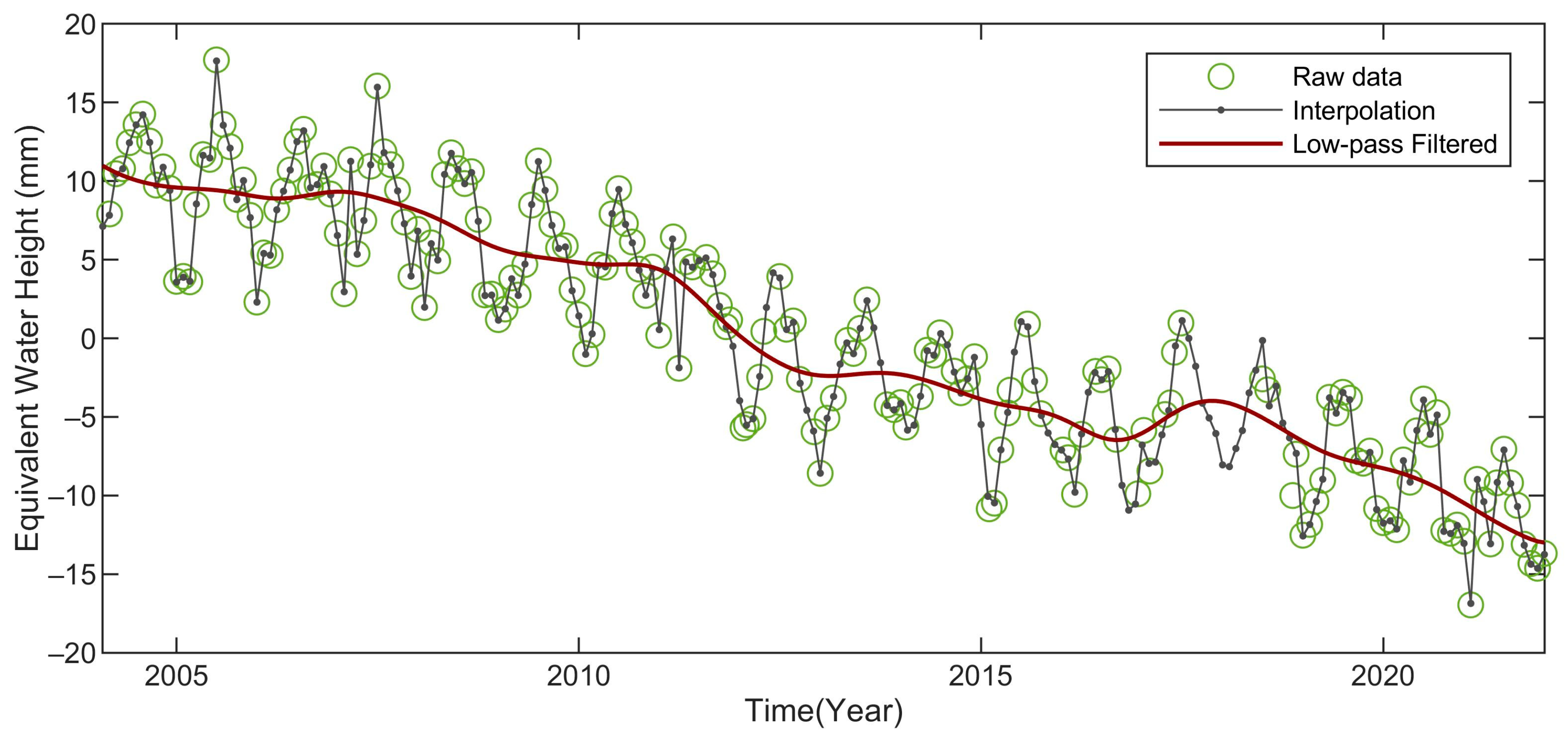
Figure 1 shows the comparison between the monthly global-mean equivalent water height anomaly time series before and after the two preprocessing steps during the study period. Figure 2 and Figure 3 illustrate the comparison between the globally distributed trends in (and peak-to-peak amplitudes of) the equivalent water height anomalies before and after the two preprocessing steps during the study period. The results show that the Lagrange interpolation and low-pass filter approaches enable reducing the noise (errors) of the GRACE/GRACE-FO mass change (Figure 3) while trying not to alter the low-frequency fluctuation patterns (including trends) in the raw data (Figure 1 and Figure 2). According to the study of Chen et al. [36], biases in GRACE/GRACE-FO-derived mass change also arise from signal leakages between land and ocean in the coastal regions surrounding Greenland, the Antarctic, southwest Alaska, and Patagonia, as well as mismodeling of the high-frequency dynamic ocean signals of the Argentine Gyre, and/or underestimating the seafloor deformation caused by great earthquakes, e.g., the Sumatra–Andaman earthquake in 2004 and the Tohoku-Oki earthquake in 2011. As shown in Figure 3b, the peak-to-peak amplitudes of the high-frequency signals near the Argentine Gyre region and other open sea regions are significantly suppressed by using a low-pass filter with a 12-month cutoff period.
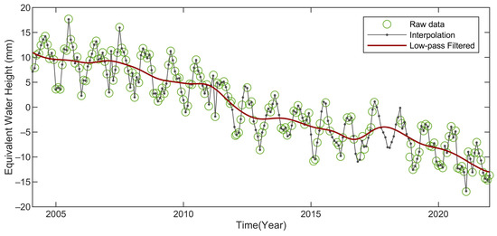
Figure 1.
Monthly global-mean equivalent water height anomalies of the raw data (green circles), data processed using Lagrange interpolation (black line with black dots), and 12-month low-pass-filtered results of interpolated data (red line) for the period January 2004 to December 2021.

Figure 2.
Globally distributed trends in gridded equivalent water height anomalies derived from GRACE/GRACE-FO data for the period January 2004 to December 2021. Trends in (a) the raw data and (b) the data processed using Lagrange interpolation and a 12-month low-pass filter. (c) The absolute difference between (a,b).

Figure 3.
Globally distributed peak-to-peak amplitudes of gridded equivalent water height anomalies derived from GRACE/GRACE-FO data for the period January 2004 to December 2021. (a) Globally distributed peak-to-peak amplitudes for the raw data; (b) is the same as (a) but for the data processed using Lagrange interpolation and a 12-month low-pass filter. (c) The absolute difference between (a,b).
2.1.2. ERA5 Reanalysis Data
To analyze the dynamic processes caused by wind-forcing and the heat gradient in regional ocean mass anomalies, the 10 m u-component of wind, the 10 m v-component of wind, and the SST data from the ERA5 monthly averaged reanalysis dataset were employed. ERA5 is the fifth generation of ECMWF reanalysis, which produces a global climate and weather dataset that is continuous in space and consistent in time by using the laws of physics to assimilate model data with the available observations from around the world [37]. The low-pass filter with a 12-month cutoff period was also applied to the ERA5 reanalysis data during the study period of January 2004 to December 2021 prior to further analysis using the GRACE/GRACE-FO-derived ocean mass anomaly data. The spatial resolution was interpolated from 0.25° × 0.25° to 0.5° × 0.5°.
2.2. Methods
The EOF method was used to analyze the spatio-temporal characteristics in TWS (and ocean water mass) anomalies based on the GRACE/GRACE-FO data. To further analyze the major drivers of ocean water mass redistribution, the MCA approach was utilized to extract the possible signals of ocean dynamic processes from the GRACE/GRACE-FO-derived ocean water mass anomalies based on the ERA5 analysis data. The sea-level equation was used to model SLFs based on the GRACE/GRACE-FO-derived TWS anomalies data. To assess the consistency between observations and estimates, two assessment indices in space and time are used, namely Pearson’s correlation coefficient and the space-similarity coefficient.
2.2.1. Empirical Orthogonal Function (EOF)
The EOF method, also known as principal component analysis (PCA), is a statistical technique used to extract matrix eigenvalues and eigenvectors, aiming to interpret large-scale, high-dimensional datasets. Lorenz [38] introduced the EOF method in the field of meteorology and climatology, and it is now widely used in physical oceanography and other fields. The eigenvectors correspond to empirical orthogonal functions (EOFs), also known as spatial modes, and the eigenvalues correspond to principal components (PCs), also known as temporal coefficients or temporal modes. These modes are ranked by the proportion of variance explained to identify the leading spatio-temporal modes of the investigated variable field. The EOF method is thus used to decompose the spatial and temporal modes or to study the major spatio-temporal evolutionary characteristics of high-dimensional data.
Given an Eulerian field with p spatial points and l time points, the field can be stored in a p × l matrix X. The EOF spatio-temporal decomposition can be expressed as follows:
where n is the total number of investigated modes, b denotes the residuals, is the t-th column of the matrix X, is the i-th leading spatial mode, and is the corresponding temporal coefficient at time t.
2.2.2. Maximum Covariance Analysis (MCA)
The MCA approach enables investigation of the coupled spatio-temporal evolutionary patterns between two variable fields, X and Y. It constructs a covariance matrix between X and Y and then performs singular value decomposition (SVD) to decompose the resulting covariance matrix into eigenvalues and eigenvectors, i.e., coupled spatio-temporal modes.
Given another Eulerian field with q spatial points and l time points, the field can be stored in a q × l matrix Y. SVD outputs the coupled spatial modes between X and Y, i.e., U and V, as follows [39]:
where is their covariance matrix, T represents the transpose of matrixes, U is a p × n matrix composed of eigenvectors whose i-th vector represents the i-th leading coupled spatial mode of X, V is a q × n matric composed of eigenvectors whose i-th vector represents the i-th leading coupled spatial mode of Y, n is the total number of investigated modes, and is a diagonal matrix whose elements on the diagonal are eigenvalues. The corresponding temporal modes and β of X and Y are then estimated based on the following equations:
The surface wind, of which the u-wind field is stored in a p × l matrix Y′ and the v-wind field is stored in a p × l matrix Y″, is reshaped as a 2p × l matrix Y before solving Equation (3). The result V is then given in a 2p × n matrix, which can be further divided into V′ and V″, which are composed of eigenvectors for the u-wind and v-wind.
2.2.3. Sea-Level Equation (SLE)
The SLE allows the estimation of relative sea level anomalies driven by changes in TWS based on the laws of physics, such as potential energy conservation and mass conservation.
The relative sea level is the ocean water column height between the surfaces of the sea and the solid Earth and is expressed as follows:
where RSL, G, and B are the anomalies at latitude , longitude , and time t, for the relative sea level, the absolute sea level (i.e., sea-surface height), and the bedrock elevation, respectively. Considering that there are differences between the actual sea-surface height and the geoid height, Equation (6) also can be rewritten as follows:
where g is the gravitational acceleration averaged over the Earth’s surface, is the net perturbation in the Earth’s surface gravitational and rotational potentials, and C is a spatial constant describing the differences between the sea-surface height and the geoid height.
Given a certain TWS anomaly field , corresponding anomalies in the globally distributed water mass load function WL can be expressed by the law of mass conservation as follows:
When TWS is known, Equation (6) to Equation (9) can be combined to solve the anomalies in the RSL caused by the land–sea water mass redistribution, i.e., SLFs and the recursion processes in the spherical harmonic domain are detailed in [11]. In this study, the input data were updated with Release 06 Version 03 of the JPL GRACE/GRACE-FO mascon data, and the SLFs were recalculated in the study period from January 2004 to December 2021.
2.2.4. Pearson’s Correlation Coefficient (PCC)
The PCC measures the similarity in temporal evolution between two variables. Given two time series, x and y, with the same sample size l, the PCC is calculated as follows [6]:
where and are the corresponding values of the i-th time point; and represent the time averages of x and y. The value of the PCC ranges from −1 to 1, with values closer to 1 indicating a higher linear correlation. A value of −1 indicates there are opposite fluctuation patterns. A value of 0 indicates that the temporal evolutionary pattern of two variables is not relevant.
2.2.5. Space-Similarity Coefficient (SC)
The SC quantifies the similarity in spatial distribution between two fields. Given two spatial distributions, Z and Z′, with the same spatial points p, the SC is calculated as follows [6]:
where and are corresponding values of the j-th spatial point, and the spatio-temporal resolution of the two input fields must be identical. The value of SC ranges from −1 to 1, with values closer to 1 indicating higher space similarity. A value of 1 indicates that the spatial distribution of the predicted and observed fields is the same, and a value of −1 indicates the exact opposite. A value of 0 indicates that the spatial distribution of two investigated fields is not relevant.
3. Results
In this section, we present the spatio-temporal characteristics of the low-frequency water mass anomalies across lands (Section 3.1.) and oceans (Section 3.2.) to discuss their relationship. Next, we illustrate the possible low-frequency dynamic ocean mass redistribution signals (Section 3.3.) and the estimated SLFs (Section 3.4.) to discuss the globally distributed contribution of different components to the GRACE/GRACE-FO-derived ocean mass anomalies (Section 3.5.).
3.1. Spatio-Temporal Evolutionary Characteristics in TWS Anomalies
This section illustrates the spatial-temporal characteristics in the GRACE/GRACE-FO-derived TWS anomalies from January 2004 to December 2021 using the EOF analysis approach. As shown in Figure 4, the first two leading modes contribute 98% of the variance explained in the raw data, and these two leading modes are associated with different time scales, namely, the long-term trend and decadal-like fluctuation.
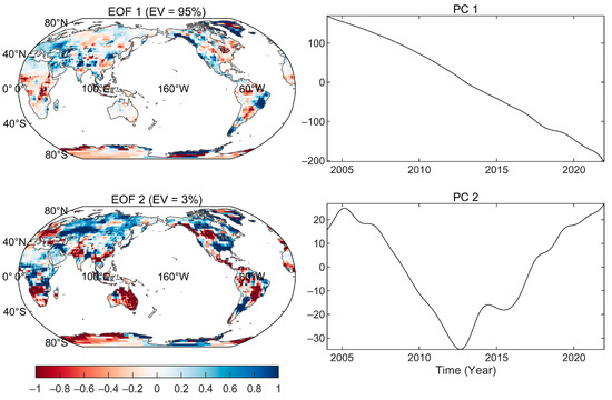
Figure 4.
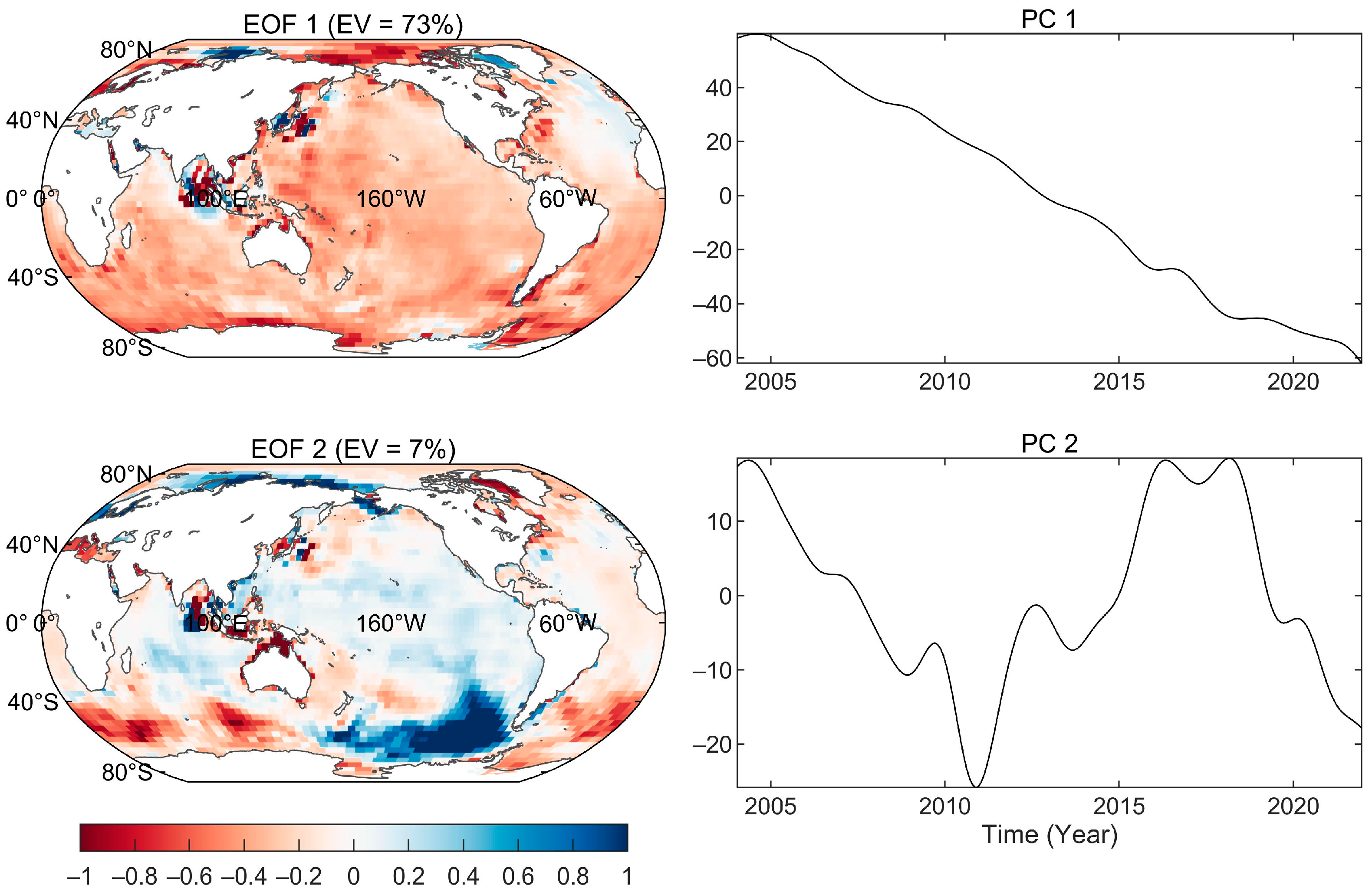
EOF analysis results of GRACE/GRACE-FO-derived TWS anomalies during the period January 2004 to December 2021. The left panel shows the EOF spatial structure, and the right panel shows the monthly time series of the corresponding PC. EOF: empirical orthogonal function; PC: principal component; EV: explained variance.
The first leading EOF mode, which mainly captures the long-term trends of the region, accounts for 95% of the variance explained in the raw data. Positive values of its EOF spatial structure, EOF1, are mainly found in the Greenland coast, the West Antarctic coast, the Alaska Range, the Coast Ranges, the South Andes Mountains, the Caucasus, the Middle East, the Qinghai-Tibet Plateau, Northern India, the North China Plain, and the Brazil Plateau, indicating that these regions experienced a significant and continuous TWS decline during the study period. In contrast, negative values of EOF1 are observed in central Greenland, the East Antarctic, eastern North America, and most low latitudes, suggesting a significant and continuous increase in TWS in these regions during the study period.
The second leading EOF mode, which captures primarily decadal-like cyclical fluctuations of the region, accounts for 3% of the variance explanation. Its EOF spatial structure, EOF2, demonstrates an inverse phase of fluctuations between the regions with positive values and the regions with negative values. Positive EOF2 values lie on the Greenland coast, the West Antarctic, northern Asia, northern and eastern North America, the Middle East, northern Africa, etc., while there are negative values for western Europe, northern India, southern Africa, Australia, the Coast Ranges, central North America, Central America, northern and Central South America, the East Antarctic, etc. The decadal-like fluctuation pattern over the regions with positive values shows an increase in TWS during the periods 2004–2005 and 2013–2021 and a TWS decline during the period 2006–2012, while that of the regions with negative values shows the opposite trend.
Combining the regional long-term trend and decadal-like fluctuation, there are two main tipping points for the regional TWS anomalies, namely, around 2005 and 2012. For instance, the Greenland coast and the West Antarctic, which are the common positive regions where both leading EOF modes are shared, show a slowing downward trend during the periods 2004–2005 and 2013–2021 and exhibit an accelerating downward trend during the period 2006–2012, which is consistent with the findings of previous studies [40,41,42,43]. The superposition of different spatio-temporal modes complicates the time-varying characteristics, and EOF analysis could be helpful for better understanding the attribution of different components involved in TWS-related ocean water mass redistribution.
3.2. Spatio-Temporal Characteristics of Ocean Water Mass Anomalies
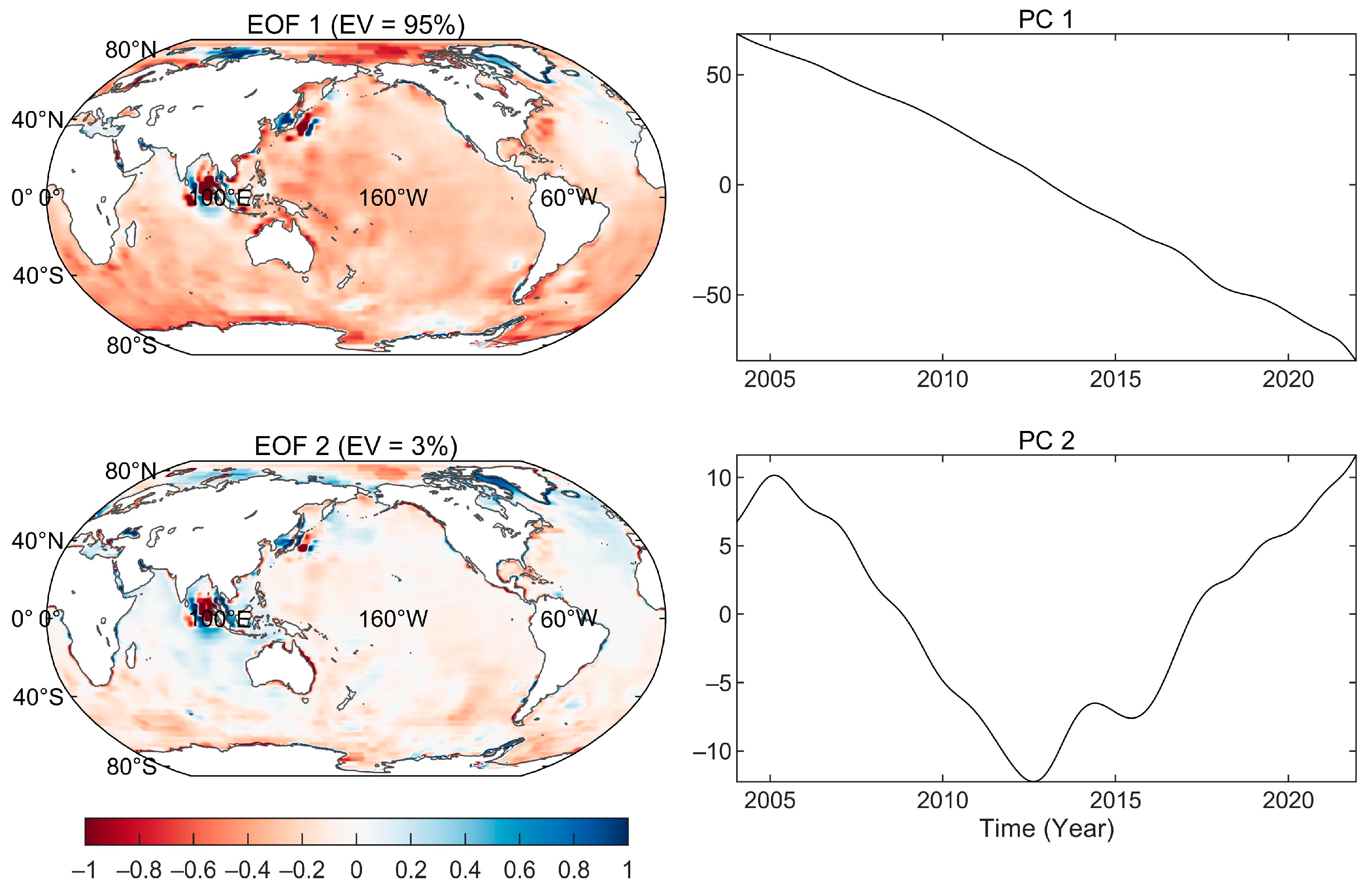
This section presents the findings of the EOF analysis method performed on GRACE/GRACE-FO-derived ocean water mass anomalies from January 2004 to December 2021. The spatio-temporal characteristics of the GRACE/GRACE-FO-derived ocean water mass anomalies are more intricate. The cumulative variance explanation of 98% in the raw data is only reached when taking into account the first to the eleventh leading spatio-temporal modes. This study focuses on the first two EOF modes, as shown in Figure 5.
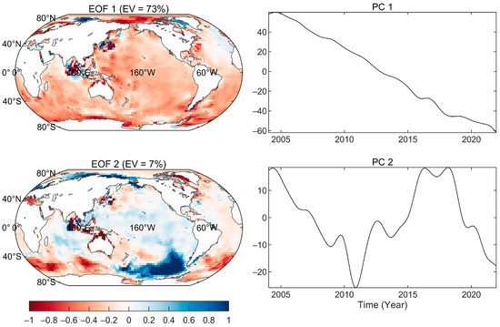
Figure 5.
EOF analysis results of GRACE/GRACE-FO-derived ocean mass anomalies during the period January 2004 to December 2021. The left panel shows the EOF spatial structure, and the right panel shows the monthly time series of the corresponding PC. EOF: empirical orthogonal function; PC: principal component; EV: explained variance.
The contribution of the first leading spatial mode, EOF1, to the variance of raw data is 73%. Its temporal mode, PC1, is dominated by a long-term trend as the PC1 of TWS, and its EOF spatial structure, EOF1, is predominantly characterized by negative values, except for the oceans surrounding Greenland and the West Antarctic, etc. This spatio-temporal evolutionary pattern is reasonable and corresponds to the overall downward trend of TWS, indicating a continued sea level rise worldwide. Sea level decline around Greenland and the West Antarctic, however, is likely a sign of SLFs.
The second leading EOF mode accounts for 7% of the variance contribution, and its temporal mode, PC2, mainly reflects decadal-like fluctuation patterns. For EOF2, the positive values of the spatial mode are mainly located in the Arctic, North Indian, and Pacific Oceans, while the negative values are mainly distributed in the Atlantic and South Indian Oceans. However, this spatial structure does not seem to respond directly to the decadal TWS fluctuations, and its PC2 time series weakly correlates with that of TWS (PCC = 0.23). Considering that high-frequency variations have been removed, EOF2 could be related to other sources of signals, e.g., low-frequency dynamic ocean water mass anomalies and/or errors in the GRACE/GRACE-FO data. For instance, strong signals of EOF2 are located in the Antarctic Circumpolar Current region, which is found to be dominated by the interannual variations in surface winds in previous studies [25,26]. Moreover, there are possible signals arising from mismodeled seafloor deformations during GRACE/GRACE-FO data preprocessing, which are located in areas where large earthquakes (e.g., the 2004 Sumatra tsunami and the 2011 Tohoku tsunami earthquakes) have occurred.
3.3. Low-Frequency Dynamic Ocean Mass Redistribution
This section uses the MCA approach to extract the possible low-frequency dynamic ocean mass redistribution signals that were driven by surface wind-forcing, heat gradients, and precipitation from the GRACE/GRACE-FO-derived ocean mass anomalies. The MCA approach outputs the possible coupled spatial-temporal modes between two variables’ fields. Only the coupled modes that are owing to strong, consistent PCs are considered in this section.
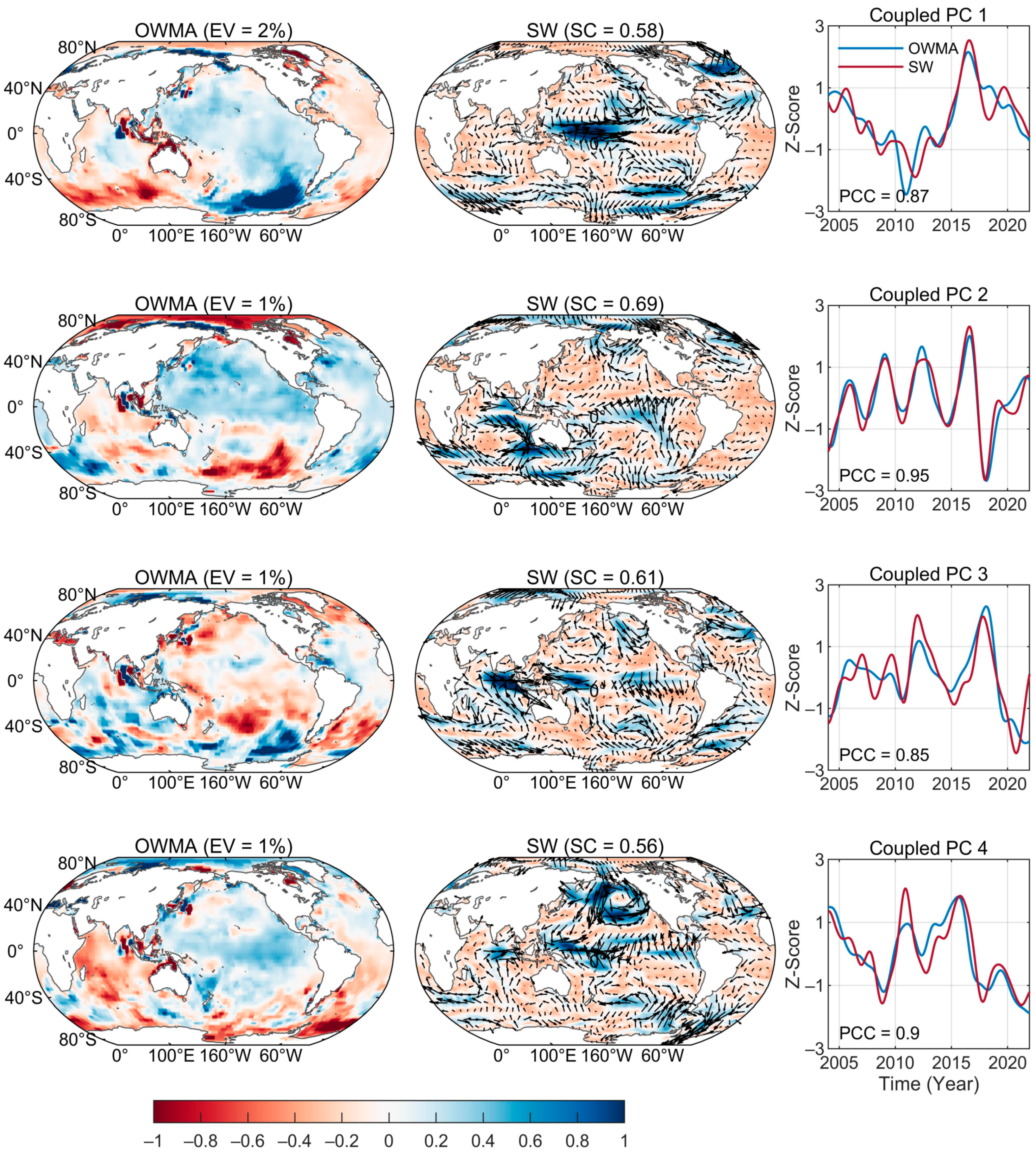
Figure 6 presents four possible spatio-temporal-coupled modes between the surface wind fields and GRACE/GRACE-FO-derived ocean mass anomaly fields during the period from January 2004 to December 2021. The SCs of their spatial modes (0.56~0.69) and the PCCs (0.85~0.95) of their temporal modes all reached a significance level of 0.05.
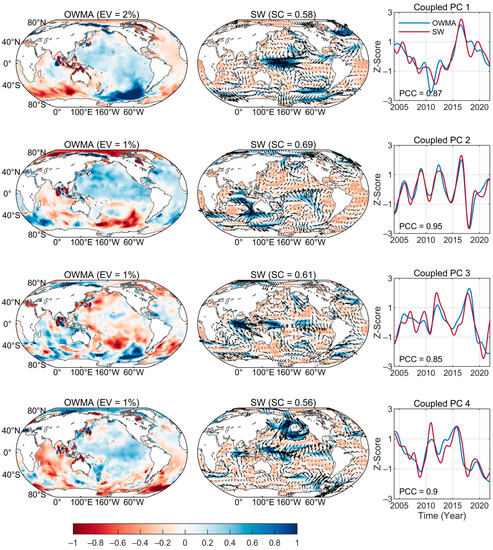
Figure 6.
Results of the maximum covariance analysis between the GRACE/GRACE-FO-derived ocean water mass anomalies and the ERA5 reanalysis-provided surface winds. Only the modes with strong, consistent PCs are shown. From left to right, the first panel shows the spatial modes (from top to bottom) of the GRACE/GRACE-FO-derived ocean water mass anomalies; the second panel shows the spatial modes (from top to bottom) of surface winds, in which shades represent wind speed anomalies relative to the global mean; and the third panel shows the time series of their coupled principal components (temporal modes) during the period January 2004 to December 2021. OWMA: ocean water mass anomaly; EV: explained variance; SW: surface wind; SC: space-similarity coefficient; PC: principal component; PCC: Pearson’s correlation coefficient.
The first coupled mode mainly illustrates a strong signal of ocean water mass anomalies across the subpolar Southern Ocean, possibly associated with decadal-like surface wind anomalies. Previous studies have found that the sea level height of the subpolar Southern Ocean is primarily driven by surface winds and is significantly correlated with ocean bottom pressure [44,45]. An anomalous wind stress along the Antarctic Circumpolar Current strongly contributes to increased water mass transport. Therefore, it is reasonable that westward (and eastward) wind anomalies correspond to ocean water mass increases (and decreases) across the subpolar Southern Ocean, as presented in the first coupled mode. Although some ocean regions also show similar patterns of decadal-like fluctuations in their surface wind field, it may not necessarily lead to a significant anomaly in the ocean water mass transport, e.g., the Equatorial-open ocean region [46].
The second coupled mode captures the ocean water mass redistribution related to the interannual wind field variations over the North Atlantic Subpolar Gyre region, the Alaska coastal current region, the Indian Ocean Gyre region, and the Australian–Antarctic Gyre region. In the North Atlantic subpolar gyre region, cyclonic (and anticyclonic) anomalies of the ocean circulation pattern that are driven by southward (and northward) wind anomalies usually lead to below-average (and above-average) Arctic Ocean water mass anomalies [27]. As shown in the second coupled spatial modes, there is a cyclonic anomaly of the surface wind field across the North Atlantic subpolar region, leading to significantly negative ocean mass anomalies of the Arctic Ocean, which is consistent with the result of [10]. The wind fields of the first and second coupled modes in the South Pacific have opposite distribution characteristics, and the corresponding South Pacific mass anomaly distribution is also opposite.
The third coupled mode captures the interannual ocean water mass redistribution that could be relevant to the wind field variations of the Equatorial marginal seas, the Alaska Gyre region, the North Pacific Subpolar Gyre region, the South Atlantic Subtropical Gyre region, and the North Atlantic Subtropical Gyre region. The fourth coupled mode further illustrates the decadal-like ocean water mass redistribution possibly driven by the wind field variations of the North Pacific Subpolar Gyre region, the Equatorial Countercurrent region, etc. Given the close relationship between the ocean mass anomalies and surface winds over these regions, the four leading coupled modes of the GRACE/GRACE-FO-derived ocean mass anomalies that are associated with surface winds (left panels of Figure 6) were removed to further study the relationship with SSTs.
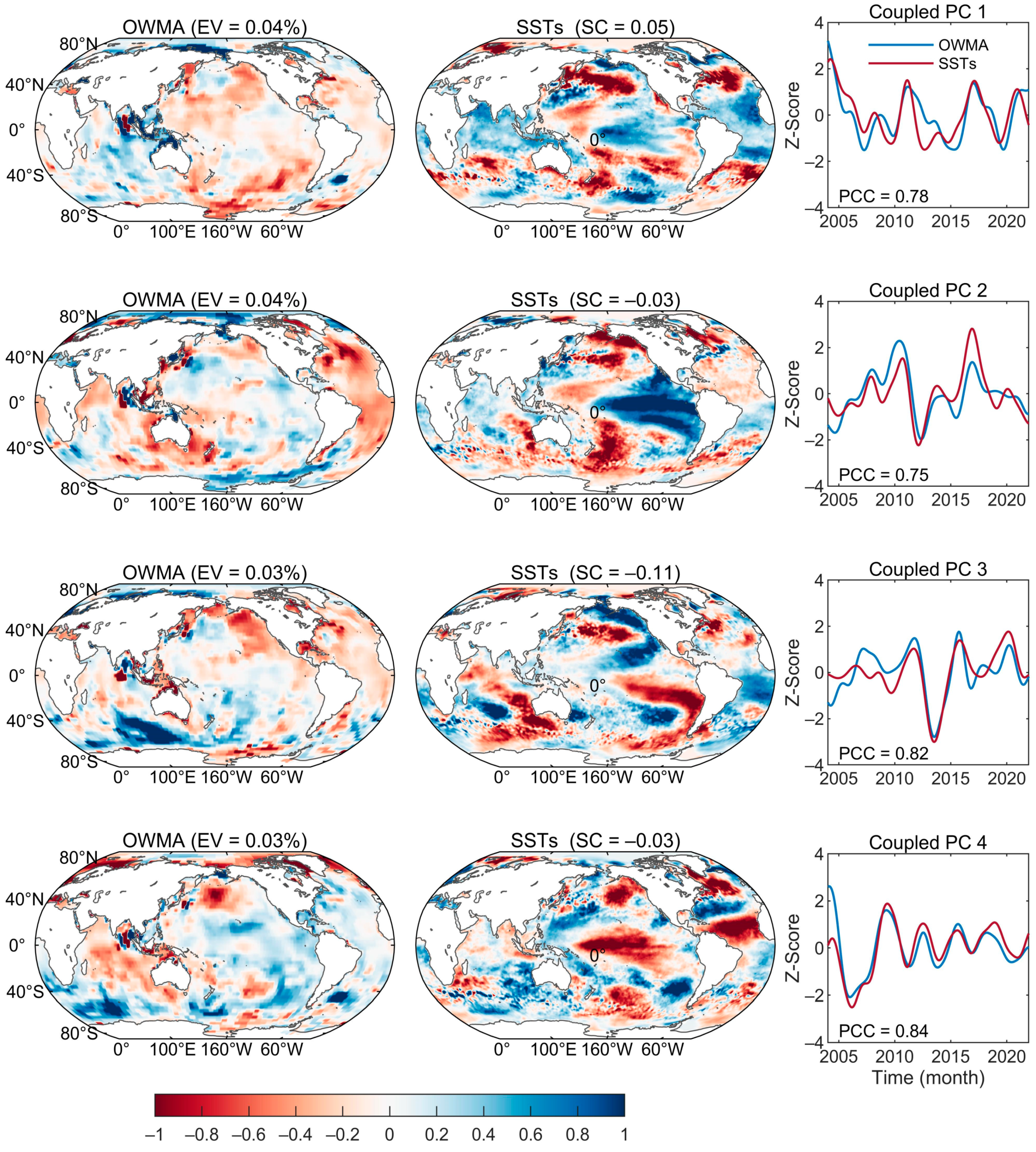
Figure 7 presents the four coupling spatial and temporal modes between the corrected GRACE/GRACE-FO-derived ocean mass anomalies and the ERA5 reanalysis-provided SSTs during the period from January 2004 to December 2021. The PCCs (0.78~0.84) between their temporal modes all reach a significance level of 0.05; however, only the SC of their third spatial-coupled modes (−0.11) passes the significance test with a p-value < 0.05. Therefore, only the third coupled modes of the GRACE/GRACE-FO-derived ocean mass anomalies that are associated with SSTs (the third left panels of Figure 7) were removed to correct the GRACE/GRACE-FO-derived ocean mass anomalies, and the signal-to-noise ratio was improved after removal. The impact of long-term precipitation variations on the residual ocean water mass anomalies was also investigated using the MCA approach to study the contribution of the water mass that is exchanged between the atmosphere and oceans, and no similar coupled spatio-temporal change pattern was found between them. The results indicate that low-frequency dynamic ocean mass anomalies are mainly caused by wind-forcing, which is consistent with the results of [10].
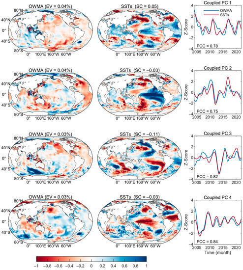
Figure 7.
Results of the maximum covariance analysis between the GRACE/GRACE-FO-derived ocean water mass anomalies and the ERA5 reanalysis-provided sea-surface temperatures (SSTs). Only the modes with strong, consistent PCs are shown. From left to right, the first panel shows the spatial modes (from top to bottom) of the GRACE/GRACE-FO-derived ocean water mass anomalies; the second panel shows the spatial modes (from top to bottom) of SSTs; and the third panel shows the time series of their coupled principal components (temporal modes) during the period January 2004 to December 2021. OWMA: ocean water mass anomaly; EV: explained variance; SC: space-similarity coefficient; PC: principal component; PCC: Pearson’s correlation coefficient.
3.4. TWS-Related Ocean Water Mass Anomalies
This section compares the modeled SLFs with the corrected GRACE/GRACE-FO-derived ocean mass anomalies when removing the possible dynamic signals to investigate TWS-related ocean water mass anomalies.
When the four leading modes of the GRACE/GRACE-FO-derived ocean mass anomalies associated with surface winds (Figure 6) and the third leading mode associated with SSTs (Figure 7) were removed, the spatio-temporal evolutionary characteristics of the ocean water mass anomalies that were related to TWS became more evident. Considering that dynamic correction may bring information from surface wind fields at a higher spatial resolution when compared with GRACE/GRACE-FO, this study further applies a Gaussian low-pass filter with a cutoff frequency of 100 to minimize very short wavelength signals after correction. Figure 8 presents the results of performing the EOF analysis on the corrected GRACE/GRACE-FO-derived ocean water mass anomalies with the oceanic dynamic processes removed. The two leading modes are highly relevant to TWS. The spatial structures of the two leading modes, EOF1 and EOF2, correspond to that of the TWS, which showed a decrease surrounding the coastal regions suffering from significant TWS decline (e.g., Greenland, Antarctic, Middle East, as shown in Figure 4), and an increase in the distance. The temporal coefficients of the two leading modes, PC1 and PC2, are in high agreement with that of TWS (PCCs ≥ 0.99). In addition, each mode explains the same variance, i.e., 95% and 3%, respectively, as shown in Figure 4 and Figure 8.
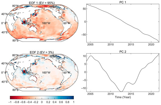
Figure 8.
EOF analysis results of GRACE/GRACE-FO-derived ocean water mass anomalies after removing the low-frequency dynamic parts during the period January 2004 to December 2021. The left panel shows the EOF spatial structure, and the right panel shows the monthly time series of the corresponding PC. EOF: empirical orthogonal function; PC: principal component; EV: explained variance. A Gaussian low-pass filter with a cutoff frequency of 100 has been applied.
Figure 9 further shows the EOF-analyzed results of the modeled SLFs during the period from January 2004 to December 2021, which describe the relative sea level anomalies driven by GRACE/GRACE-FO-derived TWS anomalies via altering Earth’s gravitation, Earth’s rotation, and solid Earth, and are calculated based on the SLE in Section 2.2.2. The first leading spatial mode of the SLFs is mainly controlled by a significant and continuous ice mass loss over the Greenland coast, the West Antarctic coast, the Alaska Range, and other coastal glacier regions. The second leading spatial mode of the SLFs is primarily determined by decadal-like TWS fluctuations over Greenland, the Antarctic, Alaska, Australia, etc. The superposition of long-term trends and decadal oscillations can lead to a sometimes accelerated and sometimes slowed sea level rise in sea level rise regions.
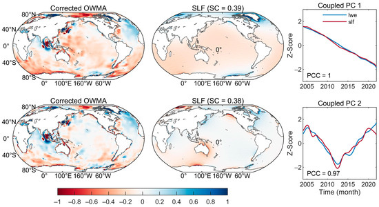
Figure 9.
Results of the maximum covariance analysis between the corrected GRACE/GRACE-FO-derived ocean water mass anomalies and the modeled SLFs. From left to right, the first panel shows the first and second leading spatial modes (from top to bottom) of the GRACE/GRACE-FO-derived ocean water mass anomalies with low-frequency ocean dynamic process removal; the second panel shows the first and second leading spatial modes (from top to bottom) of the modeled SLFs; and the third panel shows the time series of their coupled principal components (temporal modes) during the period January 2004 to December 2021. SC: space-similarity coefficient; PC: principal component; PCC: Pearson’s correlation coefficient. A Gaussian low-pass filter with a cutoff frequency of 100 has been applied in the corrected OWMA.
In this study, the modeled SLFs and the corrected GRACE/GRACE-FO-derived ocean water mass anomalies were further compared with the removal of the low-frequency dynamic ocean mass component. Although there is still some noise or signal from other sources in the corrected ocean water mass anomalies (e.g., the obvious differences being in the Arctic Ocean, the Indian Ocean near South and Southeast Asia, and the oceans surrounding the East Antarctic), the SCs between the spatial structures of the two leading modes and the PCCs between the corresponding PCs improved significantly after correction. The SCs range between approximately 0.38 and 0.39, and the PCCs range between approximately 0.97 and 1.
When the dynamic processes were removed, a visible improvement was found near the oceans surrounding Greenland and the West Antarctic. Given that the modeled SLFs have the highest gradients in the oceans near Greenland and the West Antarctic (Figure 9), the SLFs over these two regions should be more easily distinguished from the noise. As shown in Figure 10 and Figure 11, the GRACE/GRACE-FO-derived ocean mass anomalies near Greenland and the West Antarctic show an effective correction of the dynamic ocean processes, reproducing a similar pattern of gradient changes to the modeled SLFs. For oceans near Greenland, the space-similarity coefficient between the ocean mass change and SLFs improved from −0.11 to 0.58 after correction. For oceans near the West Antarctic, the space-similarity coefficient improved from 0.10 to 0.56 after correction.

Figure 10.
Comparison between the spatially distributed trends (units in mm/yr) in (a) the modeled SLFs, (b) the GRACE/GRACE-FO-derived ocean mass anomalies, and (c) the corrected GRACE/GRACE-FO-derived ocean water mass anomalies with low-frequency dynamic ocean mass redistribution removal over oceans surrounding Greenland during the period January 2004 to December 2021. A Gaussian low-pass filter with a cutoff frequency of 100 has been applied in plot-c.

Figure 11.
Comparison between the spatially distributed trends (units in mm/yr) in (a) the modeled SLFs, (b) the GRACE/GRACE-FO-derived ocean mass anomalies, and (c) the corrected GRACE/GRACE-FO-derived ocean water mass anomalies with low-frequency dynamic ocean mass redistribution removal over oceans surrounding West Antarctic during the period January 2004 to December 2021. A Gaussian low-pass filter with a cutoff frequency of 100 has been applied in plot-c.
3.5. Residuals of GRACE/GRACE-FO-Derived Ocean Mass Anomalies
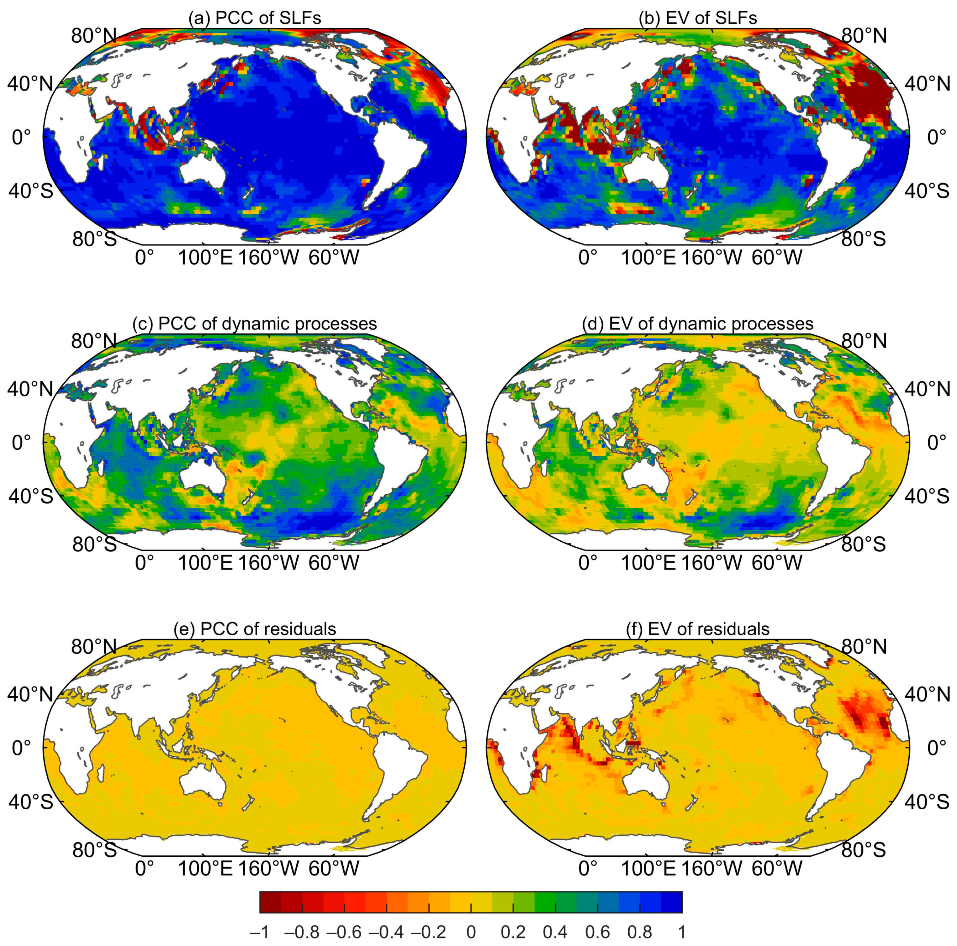
This section illustrates the globally distributed contribution of different components to the GRACE/GRACE-FO-derived ocean mass anomalies during the period from January 2004 to December 2021. As shown in Figure 12a,b, the 25th, 50th, and 75th percentiles of the PCCs between the gridded SLFs and the gridded ocean mass anomalies are 0.60, 0.86, and 0.94, respectively, while the values of the EVs are 59%, 72%, and 82%, respectively. The modeled SLFs in most regions, especially in the open ocean, have a strong correlation relationship with the GRACE/GRACE-FO-derived ocean mass anomalies, and most of them contribute more than half of the variance, indicating that the SLFs are the dominant factor causing ocean mass anomalies.
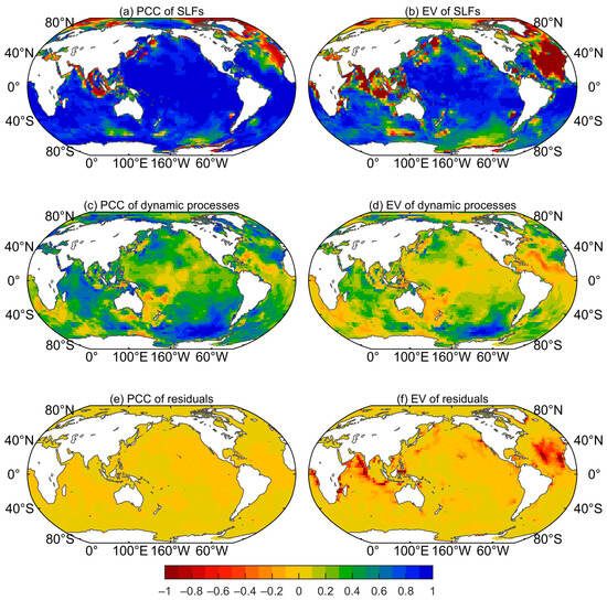
Figure 12.
Analysis of different components in the GRACE/GRACE-FO-derived ocean mass anomalies during the period January 2004 to December 2021. (a) Globally distributed correlation coefficients (PCC) between the GRACE/GRACE-FO-derived ocean mass anomalies and the modeled SLFs; (c,e) are the same as (a) but for the modeled low-frequency dynamic ocean mass redistribution and residuals, respectively. (b) Globally distributed explained variance (EV) of modeled SLFs in the GRACE/GRACE-FO-derived ocean mass anomalies; (d,f) are the same as (b) but for the modeled low-frequency dynamic ocean mass redistribution and residuals, respectively.
The second major factor causing ocean mass anomalies is the low-frequency dynamic ocean mass redistribution-forcing by surface winds and heat gradients. In Figure 12c,d, the 25th, 50th, and 75th percentiles of the PCCs between the low-frequency dynamic ocean mass anomalies and the total ocean mass anomalies in the grids are 0.22, 0.40, and 0.54, respectively, while the values of the EVs are 1%, 11%, and 23%, respectively. In the North Indian Ocean, North Atlantic Ocean, South Pacific Ocean, and some marginal seas, such as Baffin Bay, the Kara Sea, and the Laptev Sea, the low-frequency dynamic ocean mass anomalies have a high correlation with the total ocean mass anomalies, where the EVs range from 30% to 97%.
When the SLFs and the dynamic processes are deducted from the ocean mass anomalies, there is a weak correlation between the residuals and the total ocean mass anomalies (Figure 12e). However, there are non-negligible negative EVs of residuals in some regions (Figure 12f), such as the north-central Atlantic and the northern Indian Ocean. Considering the weak correlation between the residuals and the ocean water mass change, these non-negligible residuals may originate from the underestimation of magnitudes in the two investigated major components or from the dissimulated solid Earth deformation.
4. Discussion
4.1. Impact of Climate Change and Human Activities on TWS
TWS reflects the net effect of water fluxes, such as precipitation, evaporation, and runoff, and should comply with the law of regional water balance dynamics. However, in this study, it was found that the first spatial-temporal mode of TWS, dominated by trend terms, contributes 95% of the variance, which is significantly higher than the second mode, which is dominated by decadal-like fluctuations (3%) (Figure 4). Regions with decreasing trends in TWS are mostly located in glacial decline areas and groundwater overdraft areas [14,47,48,49,50,51], whereas regions exhibiting increasing trends are either undergoing a cyclical transition from dry to wet periods or experiencing increased precipitation [7,14], further indicating the dominance of climate change and human activities in terrestrial water-cycle processes.
4.2. Attribution of Ocean Water Mass Redistribution
The cumulative variance contributions of the two leading modes of TWS reach as high as 98%, and each mode corresponds to a distinct timescale variation, including long-term trends and interdecadal fluctuations. In contrast, the spatio-temporal evolution of ocean mass anomalies is more intricate, as it exhibits several distinct spatio-temporal variation patterns at similar timescales. The cumulative variance explanation of 98% in the raw data is only reached when taking into account the first to the eleventh leading spatio-temporal modes.
The main possible cause that accounts for this outcome is the low-frequency ocean dynamic processes that are involved in ocean mass redistributions. The terrestrial water cycle mainly occurs within watersheds, which have specific terrestrial boundaries and are relatively isolated [52]. Conversely, regional ocean water masses could directly interact with one another through wind-forcing or heat-related dynamic processes, given they lack physical boundaries. The results of this study show that the second leading EOF mode of ocean mass anomalies, which accounts for 7% of the explained variance (Figure 5), is in high agreement with wind-forced ocean dynamic mass anomalies (Figure 6). Previous studies have identified some ocean mass anomalies originating from wind-related dynamic processes [15]. In the Antarctic Circumpolar Current region, significant interannual variations in the ocean mass anomalies derived from GRACE have been found to be in high agreement with those of surface winds [25,26]. In the North Atlantic subpolar gyre region, ocean modeling showed that surface wind-forcing is the major driver responsible for non-seasonal water mass redistribution instead of freshwater fluxes [27]. In the North Pacific region and the Argentine Gyre region, ocean mass redistribution has also been found to be a response to low-frequency surface wind anomalies [28,29]. In this study, the global distribution of the contribution of surface winds to ocean mass anomalies was investigated, and it was concluded that wind-forcing dynamic processes dominate the ocean mass change in the North Indian Ocean, North Atlantic Ocean, South Pacific Ocean, and some marginal seas, such as Baffin Bay, the Kara Sea, and the Laptev Sea, as the variance explanations range from 30% to 97% (Figure 12d).
After removing the dynamic ocean processes, the low-frequency variations in the TWS and TWS-related ocean mass redistribution are comparable to each other in terms of the signal-to-noise rate, with their two leading modes contributing the same accumulated explained variance of 98% (Figure 4 and Figure 8). This finding further reinforces the suggestion that the GRACE/GRACE-FO-observed noise is similar in marine regions and terrestrial regions, according to the study of Chen et al. [36]. Nevertheless, it should be noted that there are non-negligible residuals remaining in the north-central Atlantic, northern Indian Ocean, etc., when the dynamic ocean processes and SLFs are removed (Figure 12f). These residuals probably originate from earthquakes. A previous study detected the transient signals of the 2004 Sumatra tsunami, the 2010 Maule tsunami, and the 2011 Tohoku tsunami earthquakes based on GRACE’s gravitational measurements [53]. With the removal of the SLFs and dynamic ocean processes, it was further found that residuals are mainly located in the seismic belt (e.g., the Circum-Pacific Belt, the mid-ocean ridge in the Indian Ocean, and the Eurasian–Melanesian belt in the Indian Ocean), which may imply the accumulated effect of numerous earthquakes on the low-frequency GRACE/GRACE-FO gravitational signals over oceanic regions. In addition, other residuals in the West Antarctic and near Greenland may be associated with leaking ice melt signals.
4.3. Comparing the SLFs Derived from Satellite Gravity and Satellite Altimetry
Recently, rapid ice melting under climate change has strengthened the signal coming from SLFs. Although detecting SLFs is challenging, recent evidence suggests that SLFs can be observed in the oceans surrounding Greenland, given the removal of ocean dynamical processes from the altimetric sea level [10]. In addition to separating the dynamic processes, an alternative approach to tracking SLFs is to remove the steric part that is associated with ocean temperature and salinity anomalies from the satellite-altimetry-derived sea level [22]. However, the latter approach only explained about 25% of the variance observed in altimetric sea level, where the correction of the steric part could be explained by SLFs. Coulson et al. [10] concluded that a correction of the steric part may perform well in the deep ocean, but the marginal seas are more likely to be dominated by ocean dynamic processes, especially the wind-forcing part. Ocean dynamic processes are reflected in the oceanic water mass anomaly rather than the steric water column height and, therefore, link the satellite gravity-derived mass sea level with the satellite altimetry-observed sea level height. As shown in Figure 10c, the satellite gravity-derived SLFs with correction of the ocean dynamic part are similar to those derived from satellite altimetry [10]. Their similar spatial distributions suggest that the sea level in the oceans off Greenland is dominated by its mass term and includes two main components, i.e., SLFs and wind-forcing ocean dynamic processes. In addition, it was further found that SLFs in the oceans that are off the West Antarctic can also be detected using a similar approach (Figure 11). These findings reinforce the suggestion that the mass term plays a dominant role in the sea level anomaly over marginal seas.
5. Conclusions
In this study, the latest version of the JPL-processed water mass anomaly dataset was used, which was derived from GRACE and GRACE-FO using the Mascon solution to investigate the major drivers of low-frequency ocean water mass redistribution during the study period from January 2004 to December 2021.
The low-pass-filtered water mass anomaly with a 12-month cutoff period in both land (TWS) and ocean were decomposed into spatial and temporal modes, respectively, using the EOF method. The results show that the first mode of TWS is dominated by the trend term and accounts for 95% of the total variance. This is followed by the second mode, which is dominated by the decadal-like fluctuation term and accounts for 3% of the total variance. The dominance of the long-term trend in TWS highlights the significant influence of climate change and human activities on the terrestrial water cycle. In contrast, the spatio-temporal evolutionary characteristics in oceans are much more complex. The first mode of ocean water mass anomalies is also dominated by the trend term but accounts for only 73% of the total variance. This is followed by the second mode, which captures mainly decadal-like fluctuations and accounts for a variance explanation of 7%. The spatio-temporal evolutions detailed in the first mode are mostly TWS-related, but those of the second mode are likely to be caused by low-frequency dynamic processes in oceans.
The ocean mass redistribution caused by dynamic processes is further revealed in their coupled spatio-temporal evolutionary modes, solved using the MCA approach. Four leading coupled modes between surface winds and ocean mass anomalies were investigated, which describe the dominant role of wind-forcing dynamic processes in the oceanic water mass anomalies near the North Indian Ocean, North Atlantic Ocean, South Pacific Ocean, and some marginal seas, such as Baffin Bay, the Kara Sea, the Laptev Sea, etc. The TWS-related ocean mass anomalies were then corrected by removing the possible dynamic processes from the raw data. By comparing the SLFs estimated using the SLE and the corrected ocean mass anomalies, it was found that the corrected ocean mass anomalies describe mostly the spatio-temporal evolutionary characteristics involved in land–sea water mass redistribution. The space-similarity coefficients of their two leading EOF modes range between approximately 0.38 and 0.39; the correlation coefficients of the corresponding PCs range between approximately 0.97 and 1; and the explained variances are the same (95% and 3%) for the long-term trend and decadal-like fluctuation terms. The residual signals probably originate from earthquake-induced seafloor deformation since they are mainly located on the seismic belt, e.g., the Circum-Pacific Belt, the mid-ocean ridge in the Indian Ocean, and the Eurasian–Melanesian belt in the Indian Ocean. This study shows that, in the low-frequency ocean water mass anomalies derived from GRACE/GRACE-FO, the contribution of the land–sea mass redistribution is the largest, followed by dynamic processes and misestimated seafloor deformation. These three driven factors provide different contributions in different regions, and caution should be taken in regional studies. Moreover, this study highlights the regions that could be dominated by wind-forcing ocean mass redistribution using the MCA approaches, offering a clue for further studying ocean dynamic processes from a mechanistic perspective at the regional to global scales.
Author Contributions
Conceptualization, S.D.; methodology, S.D., Z.J. and Y.L.; software, S.D., Z.J., and Y.L.; validation, S.D.; formal analysis, S.D.; writing—original draft preparation, S.D., Z.J., Y.L., C.Y., Y.C. and W.Z.; writing—review and editing, S.D.; visualization, S.D. All authors have read and agreed to the published version of the manuscript.
Funding
This research was funded by the National Natural Science Foundation of China (Grant No. 42201024), the Guangxi Science and Technology Program (Grant No. Guike AD23026069), the High-level Talents Project of Guangxi University (Grant No. A3100051007), and the Innovation and Entrepreneurship Training Program for College Students of Guangxi University (Grant No. 202210593060).
Data Availability Statement
JPL-processed RL06v03 GRACE and GRACE-FO mascons data are available online via https://grace.jpl.nasa.gov/data/get-data/jpl_global_mascons/, accessed on 12 June 2023 and the JPL GRACE/GRACE-FO Gridded-AOD1B Water-Equivalent-Thickness Surface-Mass Anomaly RL06 dataset for the Tellus Level-3 mascon 0.5-degree are available online via https://podaac.jpl.nasa.gov/dataset/GRC-GFO_GRIDDED_AOD1B_JPL_MASCON_RL06, accessed on 13 June 2023. ERA5 reanalysis data are available online via https://cds.climate.copernicus.eu/cdsapp#!/dataset/reanalysis-era5-single-levels-monthly-means?tab=form, accessed on 13 June 2023.
Acknowledgments
The authors are thankful to Chad A. Greene from the University of Texas Institute for Geophysics (UTIG) for creating the “eof” function with MATLAB codes.
Conflicts of Interest
The authors declare no conflict of interest.
References
- Deng, S.; Liu, S.; Mo, X.; Jiang, L.; Bauer-Gottwein, P. Polar drift in the 1990s explained by terrestrial water storage changes. Geophys. Res. Lett. 2021, 48, e2020GL092114. [Google Scholar] [CrossRef]
- Deng, S.; Liu, Y.; Zhang, W. A Comprehensive Evaluation of GRACE-Like Terrestrial Water Storage (TWS) Reconstruction Products at an Interannual Scale During 1981–2019. Water Resour. Res. 2023, 59, e2022WR034381. [Google Scholar] [CrossRef]
- Frederikse, T.; Landerer, F.; Caron, L.; Adhikari, S.; Parkes, D.; Humphrey, V.W.; Dangendorf, S.; Hogarth, P.; Zanna, L.; Cheng, L.; et al. The causes of sea-level rise since 1900. Nature 2020, 584, 393–397. [Google Scholar] [CrossRef] [PubMed]
- IPCC. Climate Change 2021: The Physical Science Basis; Douville, H., Raghavan, K., Renwick, J., Eds.; Cambridge University Press: Cambridge, UK, 2021. [Google Scholar]
- Seo, K.-W.; Ryu, D.; Eom, J.; Jeon, T.; Kim, J.-S.; Youm, K.; Chen, J.; Wilson, C.R. Drift of Earth’s Pole Confirms Groundwater Depletion as a Significant Contributor to Global Sea Level Rise 1993–2010. Geophys. Res. Lett. 2023, 50, e2023GL103509. [Google Scholar] [CrossRef]
- Deng, S.; Liu, S.; Mo, X. Assessment of Three Common Methods for Estimating Terrestrial Water Storage Change with Three Reanalysis Datasets. J. Clim. 2020, 33, 511–525. [Google Scholar] [CrossRef]
- Deng, S.; Liu, S.; Mo, X. Assessment and attribution of China’s droughts using an integrated drought index derived from GRACE and GRACE-FO data. J. Hydrol. 2021, 603, 127170. [Google Scholar] [CrossRef]
- Farrell, W.E.; Clark, J.A. On Postglacial Sea Level. Geophys. J. R. Astron. Soc. 1976, 46, 647–667. [Google Scholar] [CrossRef]
- Haubrich, R., Jr.; Munk, W. The pole tide. J. Geophys. Res. 1959, 64, 2373–2388. [Google Scholar] [CrossRef]
- Coulson, S.; Dangendorf, S.; Mitrovica, J.X.; Tamisiea, M.E.; Pan, L.; Sandwell, D.T. A detection of the sea level fingerprint of Greenland Ice Sheet melt. Science 2022, 377, 1550–1554. [Google Scholar] [CrossRef]
- Adhikari, S.; Ivins, E.R.; Frederikse, T.; Landerer, F.W.; Caron, L. Sea-level fingerprints emergent from GRACE mission data. Earth Syst. Sci. Data 2019, 11, 629–646. [Google Scholar] [CrossRef]
- Gregory, J.M.; Griffies, S.M.; Hughes, C.W.; Lowe, J.A.; Church, J.A.; Fukimori, I.; Gomez, N.; Kopp, R.E.; Landerer, F.; Cozannet, G.L.; et al. Concepts and Terminology for Sea Level: Mean, Variability and Change, Both Local and Global. Surv. Geophys. 2019, 40, 1251–1289. [Google Scholar] [CrossRef]
- Volkov, D.L.; Lee, S.-K.; Landerer, F.W.; Lumpkin, R. Decade-long deep-ocean warming detected in the subtropical South Pacific. Geophys. Res. Lett. 2017, 44, 927–936. [Google Scholar] [CrossRef] [PubMed]
- Rodell, M.; Famiglietti, J.S.; Wiese, D.N.; Reager, J.T.; Beaudoing, H.K.; Landerer, F.W.; Lo, M.H. Emerging trends in global freshwater availability. Nature 2018, 557, 651–659. [Google Scholar] [CrossRef] [PubMed]
- Tapley, B.D.; Watkins, M.M.; Flechtner, F.; Reigber, C.; Bettadpur, S.; Rodell, M.; Sasgen, I.; Famiglietti, J.S.; Landerer, F.W.; Chambers, D.P.; et al. Contributions of GRACE to understanding climate change. Nat. Clim. Chang. 2019, 9, 358–369. [Google Scholar] [CrossRef]
- Gornitz, V. Global coastal hazards from future sea level rise. Palaeogeogr. Palaeoclimatol. Palaeoecol. 1991, 89, 379–398. [Google Scholar] [CrossRef]
- Hauer, M.E.; Fussell, E.; Mueller, V.; Burkett, M.; Call, M.; Abel, K.; McLeman, R.; Wrathall, D. Sea-level rise and human migration. Nat. Rev. Earth Environ. 2020, 1, 28–39. [Google Scholar] [CrossRef]
- Melet, A.; Teatini, P.; Le Cozannet, G.; Jamet, C.; Conversi, A.; Benveniste, J.; Almar, R. Earth Observations for Monitoring Marine Coastal Hazards and Their Drivers. Surv. Geophys. 2020, 41, 1489–1534. [Google Scholar] [CrossRef]
- Tapley, B.D.; Bettadpur, S.; Watkins, M.; Reigber, C. The gravity recovery and climate experiment: Mission overview and early results. Geophys. Res. Lett. 2004, 31. [Google Scholar] [CrossRef]
- Hsu, C.-W.; Velicogna, I. Detection of sea level fingerprints derived from GRACE gravity data. Geophys. Res. Lett. 2017, 44, 8953–8961. [Google Scholar] [CrossRef]
- Jeon, T.; Seo, K.-W.; Kim, B.-H.; Kim, J.-S.; Chen, J.; Wilson, C.R. Sea level fingerprints and regional sea level change. Earth Planet. Sci. Lett. 2021, 567, 116985. [Google Scholar] [CrossRef]
- Moreira, L.; Cazenave, A.; Barnoud, A.; Chen, J. Sea-Level Fingerprints Due to Present-Day Water Mass Redistribution in Observed Sea-Level Data. Remote Sens. 2021, 13, 4667. [Google Scholar] [CrossRef]
- Uebbing, B.; Rietbroek, R.; Kusche, J. Investigating global and regional sea level budgets by combining GRACE (-FO) and altimetry data in a joint fingerprint inversion. In Proceedings of the EGU General Assembly Conference Abstracts, Vienna, Austria, 23–27 May 2022; p. EGU22-2190. [Google Scholar]
- Rietbroek, R.; Brunnabend, S.-E.; Kusche, J.; Schröter, J.; Dahle, C. Revisiting the contemporary sea-level budget on global and regional scales. Proc. Natl. Acad. Sci. USA 2016, 113, 1504–1509. [Google Scholar] [CrossRef] [PubMed]
- Zlotnicki, V.; Wahr, J.; Fukumori, I.; Song, Y.T. Antarctic Circumpolar Current Transport Variability during 2003–05 from GRACE. J. Phys. Oceanogr. 2007, 37, 230–244. [Google Scholar] [CrossRef]
- Bergmann, I.; Dobslaw, H. Short-term transport variability of the Antarctic Circumpolar Current from satellite gravity observations. J. Geophys. Res. Ocean. 2012, 117, C5. [Google Scholar] [CrossRef]
- Volkov, D.L.; Landerer, F.W. Nonseasonal fluctuations of the Arctic Ocean mass observed by the GRACE satellites. J. Geophys. Res. Ocean. 2013, 118, 6451–6460. [Google Scholar] [CrossRef]
- Petrick, C.; Dobslaw, H.; Bergmann-Wolf, I.; Schön, N.; Matthes, K.; Thomas, M. Low-frequency ocean bottom pressure variations in the North Pacific in response to time-variable surface winds. J. Geophys. Res. Ocean. 2014, 119, 5190–5202. [Google Scholar] [CrossRef]
- Yu, Y.; Chao, B.F.; García-García, D.; Luo, Z. Variations of the Argentine Gyre Observed in the GRACE Time-Variable Gravity and Ocean Altimetry Measurements. J. Geophys. Res. Ocean. 2018, 123, 5375–5387. [Google Scholar] [CrossRef]
- Rietbroek, R. Retrieval of Sea Level and Surface Loading Variations from Geodetic Observations and Model Simulations. Ph.D. Thesis, Universitäts-und Landesbibliothek Bonn, Bonn, Germany, 2014. [Google Scholar]
- Sun, Y.; Riva, R.; Ditmar, P.; Rietbroek, R. Using GRACE to explain variations in the Earth’s oblateness. Geophys. Res. Lett. 2019, 46, 158–168. [Google Scholar] [CrossRef]
- Landerer, F.W.; Flechtner, F.M.; Save, H.; Webb, F.H.; Bandikova, T.; Bertiger, W.I.; Bettadpur, S.V.; Byun, S.H.; Dahle, C.; Dobslaw, H.; et al. Extending the Global Mass Change Data Record: GRACE Follow-On Instrument and Science Data Performance. Geophys. Res. Lett. 2020, 47, e2020GL088306. [Google Scholar] [CrossRef]
- Peltier, W.R.; Argus, D.F.; Drummond, R. Comment on “An Assessment of the ICE-6G_C (VM5a) Glacial Isostatic Adjustment Model” by Purcell et al. J. Geophys. Res. Solid Earth 2018, 123, 2019–2028. [Google Scholar] [CrossRef]
- Watkins, M.M.; Wiese, D.N.; Yuan, D.-N.; Boening, C.; Landerer, F.W. Improved methods for observing Earth’s time variable mass distribution with GRACE using spherical cap mascons. J. Geophys. Res. Solid Earth 2015, 120, 2648–2671. [Google Scholar] [CrossRef]
- Wiese, D.N.; Landerer, F.W.; Watkins, M.M. Quantifying and reducing leakage errors in the JPL RL05M GRACE mascon solution. Water Resour. Res. 2016, 52, 7490–7502. [Google Scholar] [CrossRef]
- Chen, J.; Tapley, B.; Tamisiea, M.E.; Save, H.; Wilson, C.; Bettadpur, S.; Seo, K.-W. Error Assessment of GRACE and GRACE Follow-On Mass Change. J. Geophys. Res. Solid Earth 2021, 126, e2021JB022124. [Google Scholar] [CrossRef]
- Hersbach, H.; Bell, B.; Berrisford, P.; Hirahara, S.; Horányi, A.; Muñoz-Sabater, J.; Nicolas, J.; Peubey, C.; Radu, R.; Schepers, D.; et al. The ERA5 global reanalysis. Q. J. R. Meteorol. Soc. 2020, 146, 1999–2049. [Google Scholar] [CrossRef]
- Lorenz, E.N. Empirical Orthogonal Functions and Statistical Weather Prediction; Massachusetts Institute of Technology, Department of Meteorology: Cambridge, MA, USA, 1956; Volume 1. [Google Scholar]
- Barreto, N.J.C.; Mesquita, M.d.S.; Mendes, D.; Spyrides, M.H.C.; Pedra, G.U.; Lucio, P.S. Maximum covariance analysis to identify intraseasonal oscillations over tropical Brazil. Clim. Dyn. 2017, 49, 1583–1596. [Google Scholar] [CrossRef]
- Chen, J.; Wilson, C.; Tapley, B. Satellite gravity measurements confirm accelerated melting of Greenland ice sheet. Science 2006, 313, 1958–1960. [Google Scholar] [CrossRef]
- Velicogna, I. Increasing rates of ice mass loss from the Greenland and Antarctic ice sheets revealed by GRACE. Geophys. Res. Lett. 2009, 36, L19503. [Google Scholar] [CrossRef]
- Rignot, E.; Velicogna, I.; van den Broeke, M.R.; Monaghan, A.; Lenaerts, J.T. Acceleration of the contribution of the Greenland and Antarctic ice sheets to sea level rise. Geophys. Res. Lett. 2011, 38, L05503. [Google Scholar] [CrossRef]
- Sasgen, I.; Wouters, B.; Gardner, A.S.; King, M.D.; Tedesco, M.; Landerer, F.W.; Dahle, C.; Save, H.; Fettweis, X. Return to rapid ice loss in Greenland and record loss in 2019 detected by the GRACE-FO satellites. Commun. Earth Environ. 2020, 1, 8. [Google Scholar] [CrossRef]
- Piecuch, C.G.; Quinn, K.J.; Ponte, R.M. Satellite-derived interannual ocean bottom pressure variability and its relation to sea level. Geophys. Res. Lett. 2013, 40, 3106–3110. [Google Scholar] [CrossRef]
- Naveira Garabato, A.C.; Dotto, T.S.; Hooley, J.; Bacon, S.; Tsamados, M.; Ridout, A.; Frajka-Williams, E.E.; Herraiz-Borreguero, L.; Holland, P.R.; Heorton, H.D.B.S.; et al. Phased Response of the Subpolar Southern Ocean to Changes in Circumpolar Winds. Geophys. Res. Lett. 2019, 46, 6024–6033. [Google Scholar] [CrossRef]
- Delforge, D.; de Viron, O.; Durand, F.; Dehant, V. The Global Patterns of Interannual and Intraseasonal Mass Variations in the Oceans from GRACE and GRACE Follow-On Records. Remote Sens. 2022, 14, 1861. [Google Scholar] [CrossRef]
- Zavialov, P.; Kostianoy, A.; Emelianov, S.; Ni, A.; Ishniyazov, D.; Khan, V.; Kudyshkin, T. Hydrographic survey in the dying Aral Sea. Geophys. Res. Lett. 2003, 30, 1659. [Google Scholar] [CrossRef]
- Rodell, M.; Velicogna, I.; Famiglietti, J.S. Satellite-based estimates of groundwater depletion in India. Nature 2009, 460, 999–1002. [Google Scholar] [CrossRef] [PubMed]
- Voss, K.A.; Famiglietti, J.S.; Lo, M.H.; de Linage, C.; Rodell, M.; Swenson, S.C. Groundwater depletion in the Middle East from GRACE with implications for transboundary water management in the Tigris-Euphrates-Western Iran region. Water Resour. Res. 2013, 49, 904–914. [Google Scholar] [CrossRef]
- Wang, J.; Song, C.; Reager, J.T.; Yao, F.; Famiglietti, J.S.; Sheng, Y.; MacDonald, G.M.; Brun, F.; Schmied, H.M.; Marston, R.A.; et al. Recent global decline in endorheic basin water storages. Nat. Geosci. 2018, 11, 926–932. [Google Scholar] [CrossRef]
- Zemp, M.; Huss, M.; Thibert, E.; Eckert, N.; McNabb, R.; Huber, J.; Barandun, M.; Machguth, H.; Nussbaumer, S.U.; Gärtner-Roer, I.; et al. Global glacier mass changes and their contributions to sea-level rise from 1961 to 2016. Nature 2019, 568, 382–386. [Google Scholar] [CrossRef]
- Cheng, G.D.; Li, X. Integrated research methods in watershed science. Sci. China Earth Sci. 2015, 58, 1159–1168. [Google Scholar] [CrossRef]
- Ghobadi-Far, K.; Han, S.-C.; Allgeyer, S.; Tregoning, P.; Sauber, J.; Behzadpour, S.; Mayer-Gürr, T.; Sneeuw, N.; Okal, E. GRACE gravitational measurements of tsunamis after the 2004, 2010, and 2011 great earthquakes. J. Geod. 2020, 94, 65. [Google Scholar] [CrossRef]
Disclaimer/Publisher’s Note: The statements, opinions and data contained in all publications are solely those of the individual author(s) and contributor(s) and not of MDPI and/or the editor(s). MDPI and/or the editor(s) disclaim responsibility for any injury to people or property resulting from any ideas, methods, instructions or products referred to in the content. |
© 2023 by the authors. Licensee MDPI, Basel, Switzerland. This article is an open access article distributed under the terms and conditions of the Creative Commons Attribution (CC BY) license (https://creativecommons.org/licenses/by/4.0/).

