
Variations in Phenology Identification Strategies across the Mongolian Plateau Using Multiple Data Sources and Methods


Abstract
:
1. Introduction
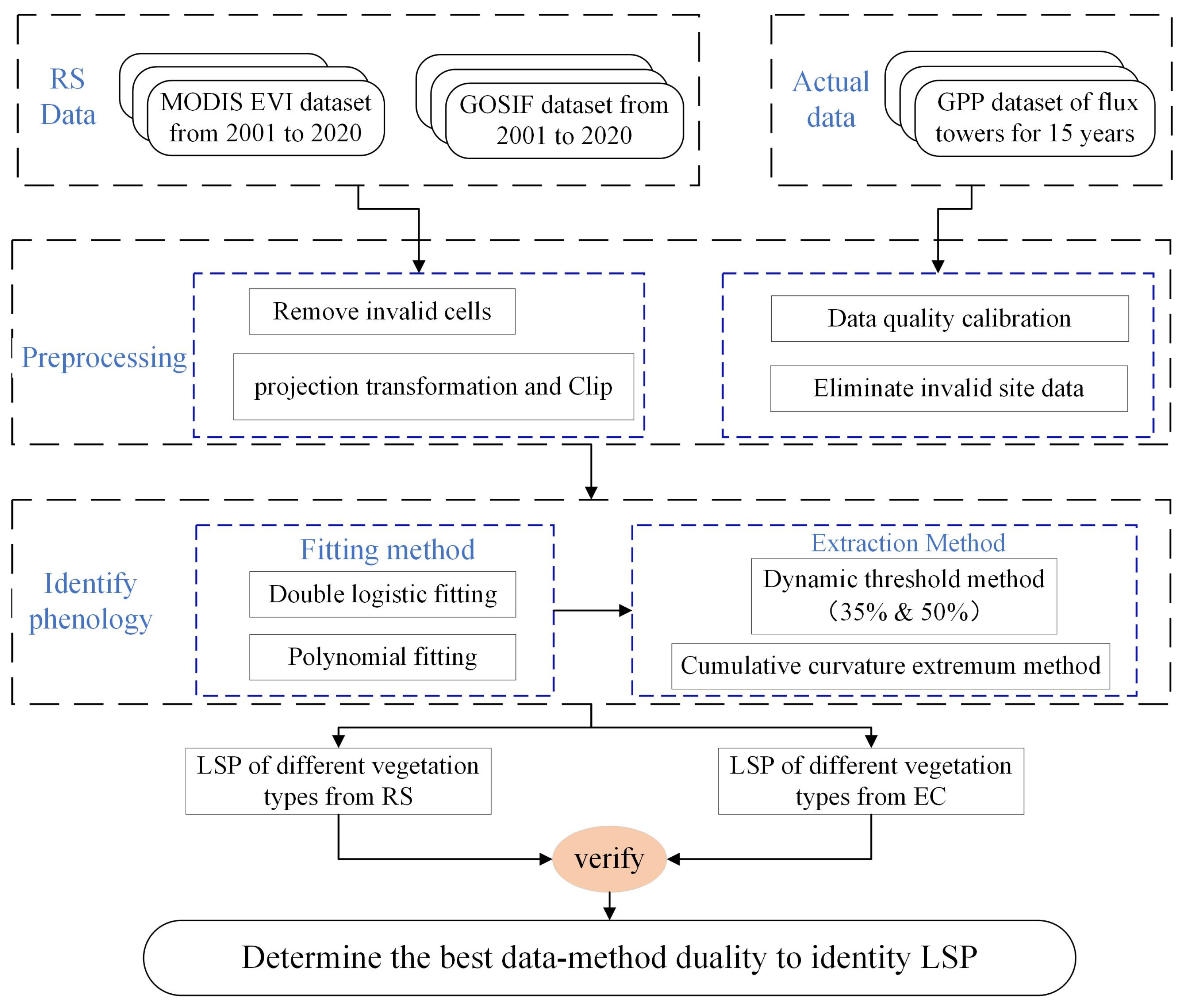
2. Materials and Methods
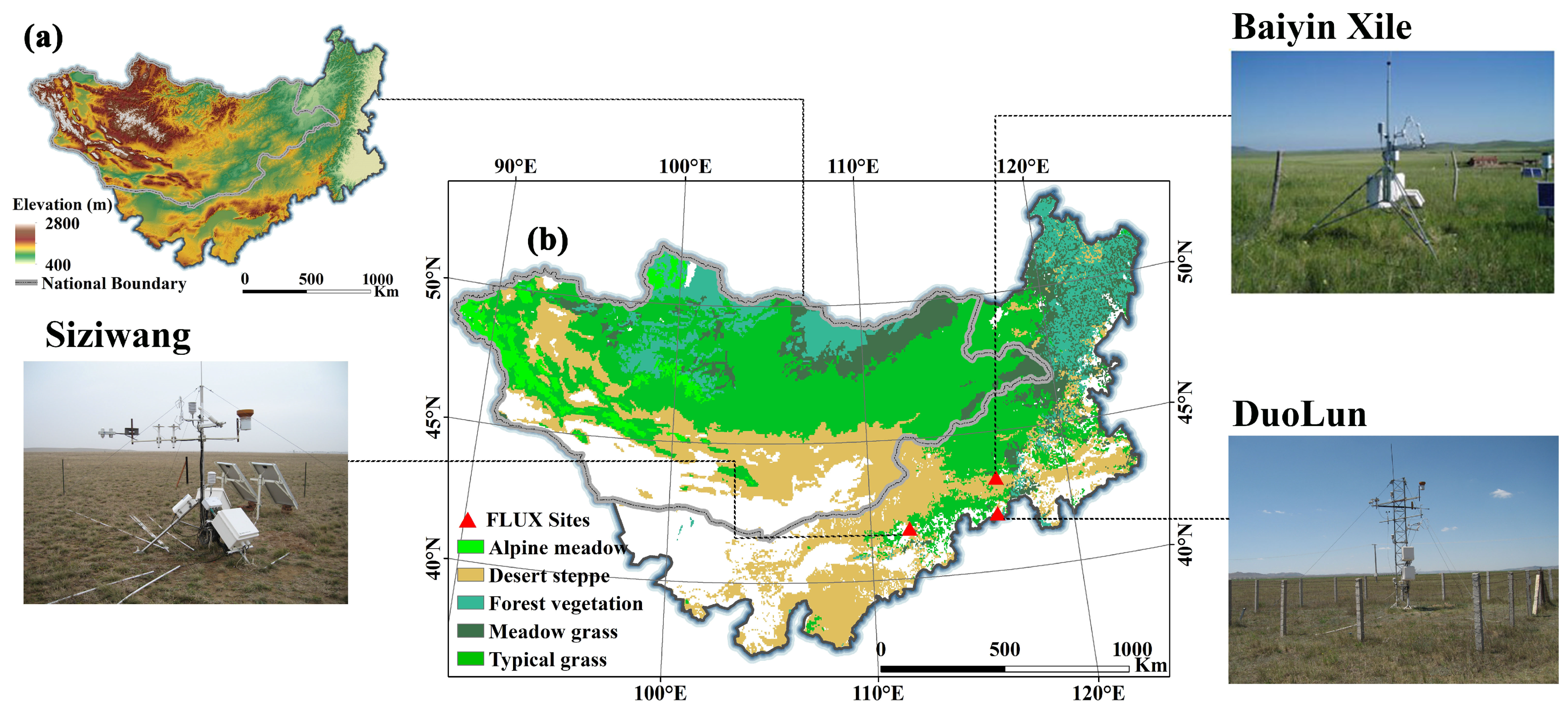
2.1. Study Area
2.2. Data Sources
2.2.1. Eddy Covariance Flux Data
2.2.2. Remote Sensing Data
2.3. Methods
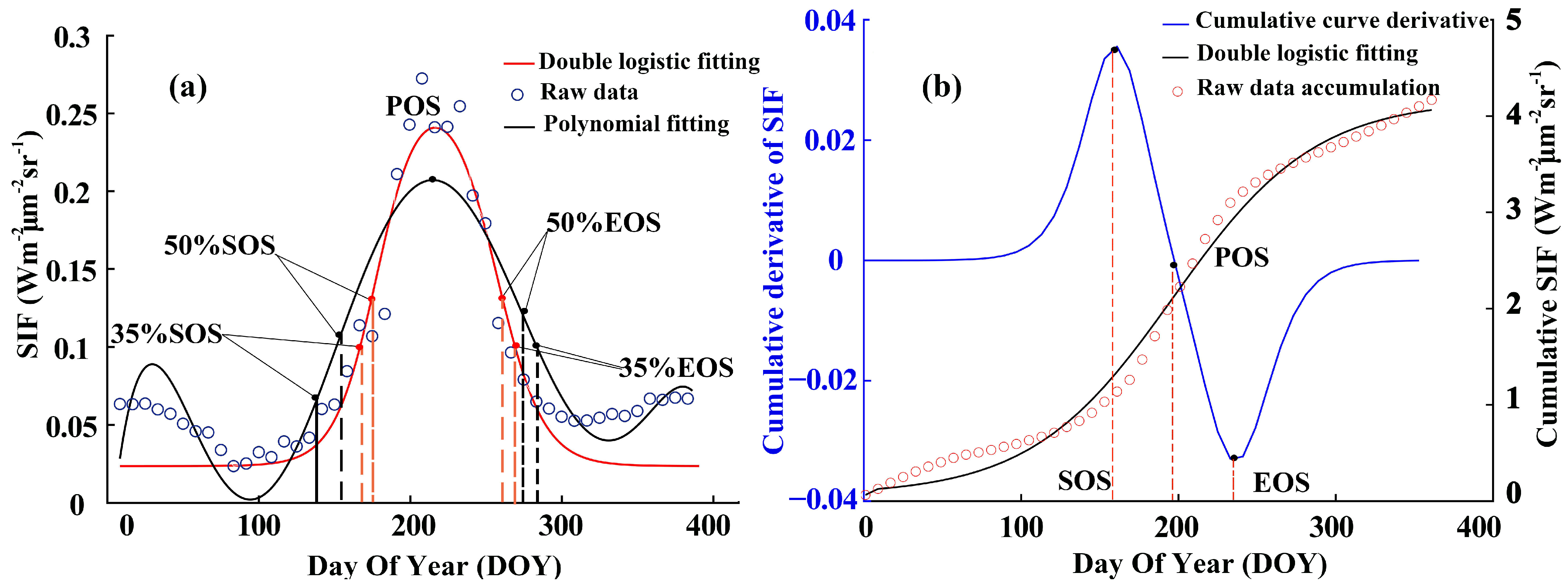
2.3.1. Phenology Extraction Algorithms
- (1)
- DL-G35
- (2)
- DL-G50
- (3)
- Poly-G35
- (4)
- Poly-G50
- (5)
- DL-CUM
2.3.2. Evaluation of Land Surface Phenology Retrieval Algorithm
3. Results
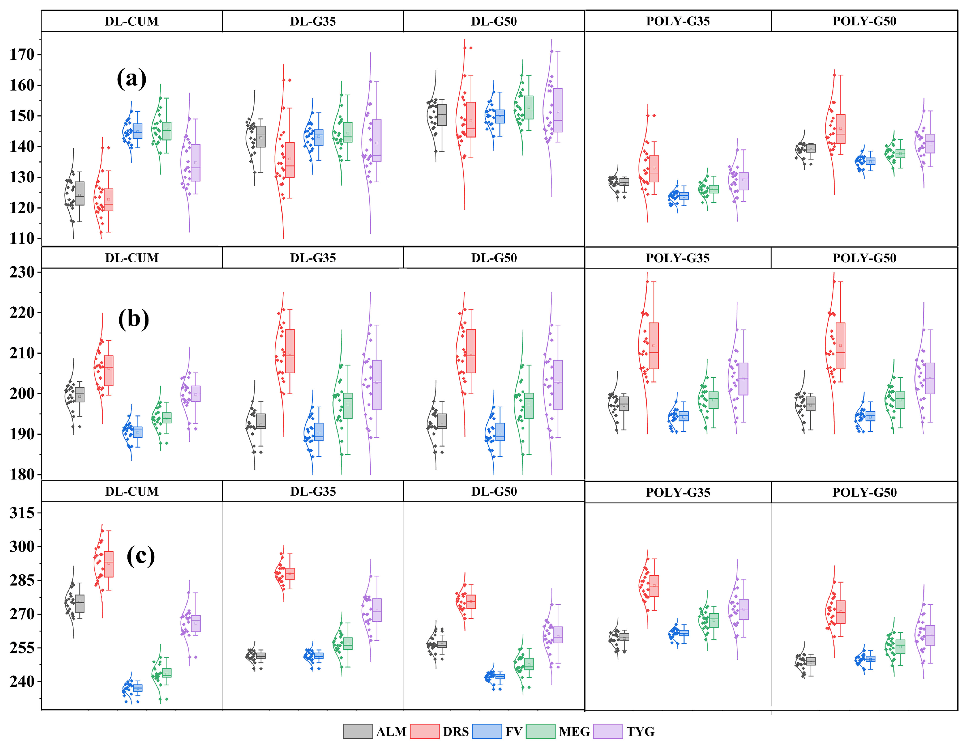
3.1. Evaluation of Land Surface Phenology Retrieval Data and Algorithms
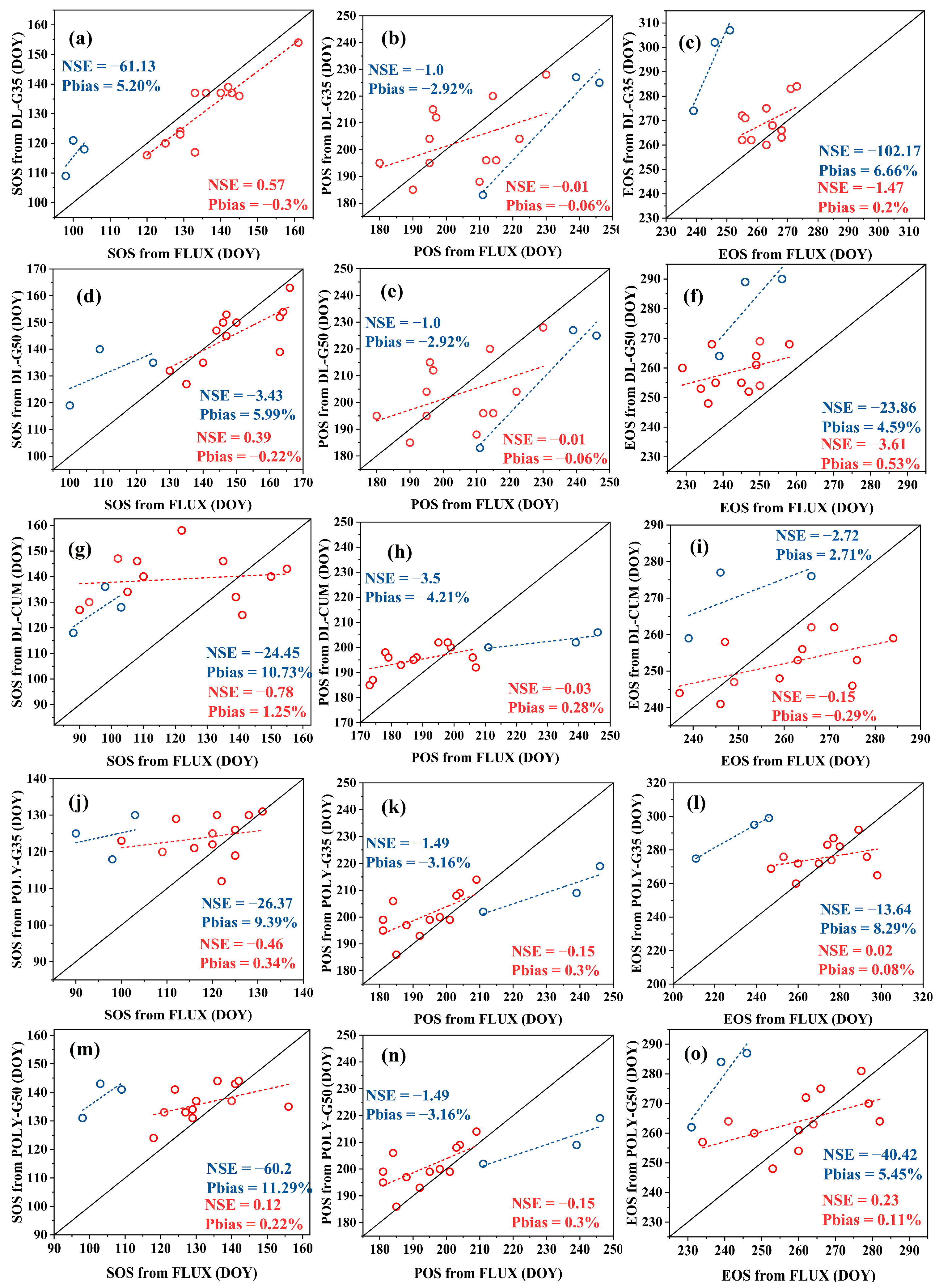
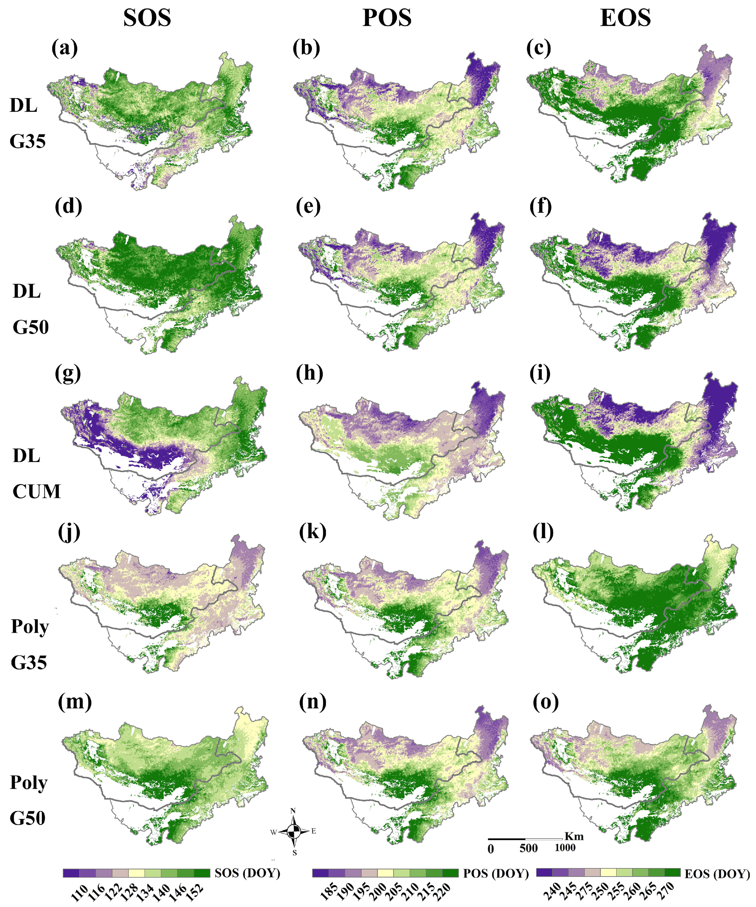
3.2. Phenology Estimated from EVI
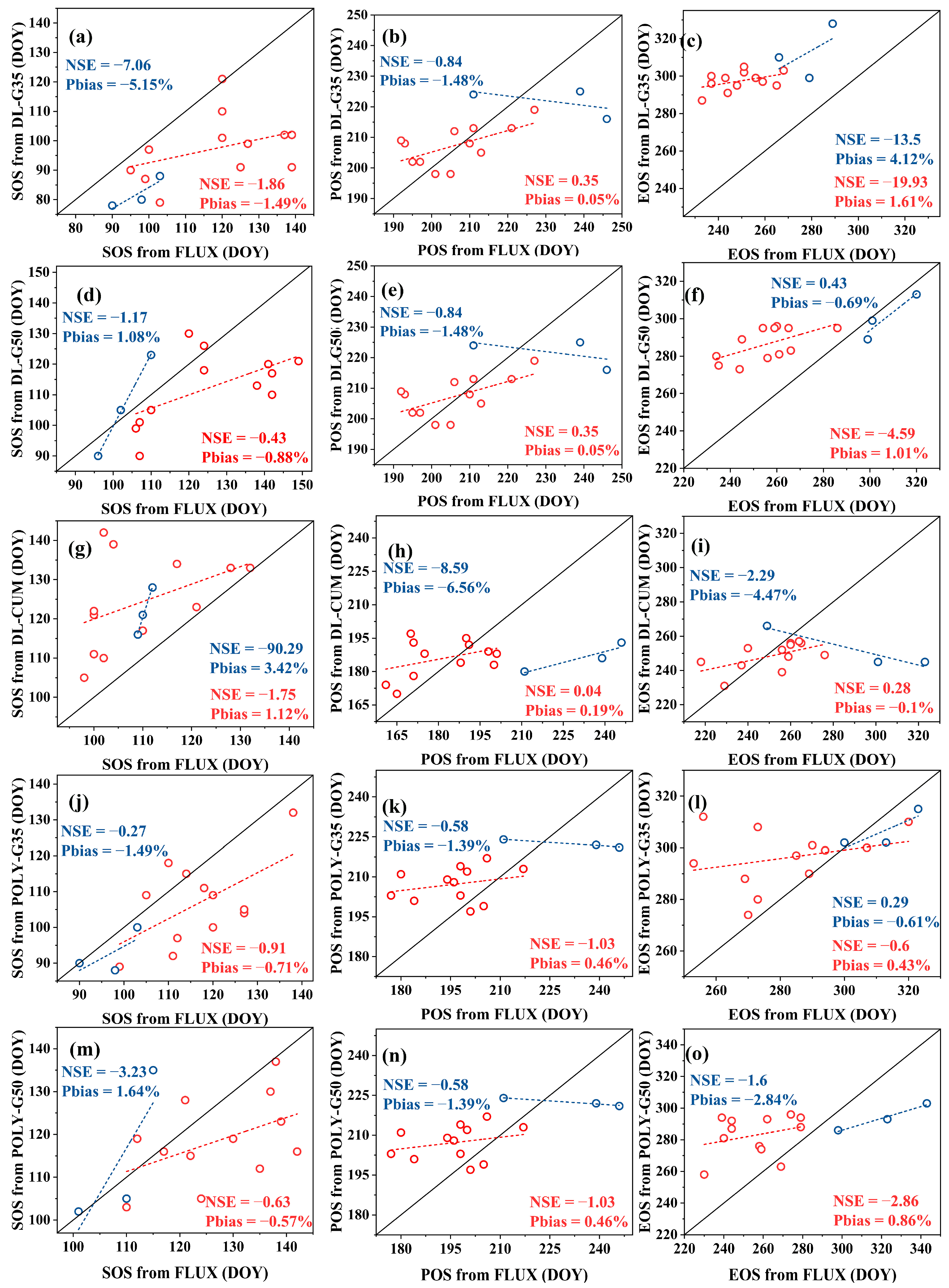
3.3. Phenology Estimated from SIF
4. Discussion
4.1. Algorithm and Data Performance
4.2. Limitations and Prospects
5. Conclusions
- (1)
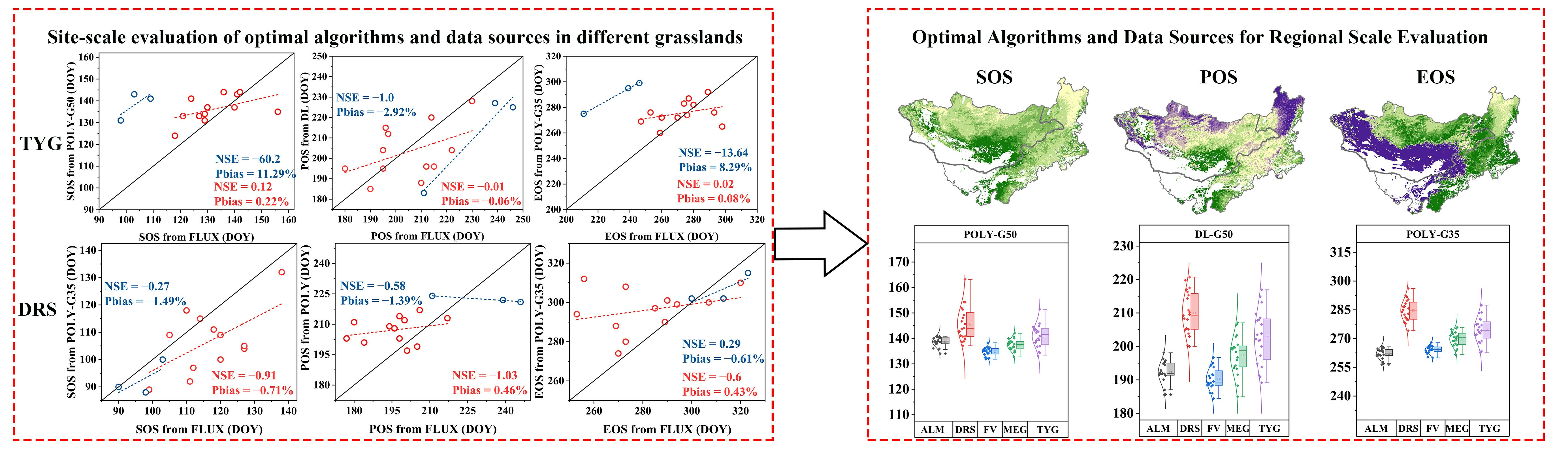
- The optimal methods for identifying the SOS, POS, and EOS of typical grassland areas were Poly-G50 (NSE = 0.12, Pbias = 0.22%), DL-G35/50 (NSE = −0.01, Pbias = −0.06%), and Poly-G35 (NSE = 0.02, Pbias = 0.08%), respectively, based on SIF data. The best methods for identifying the SOS, POS, and EOS of desert steppe areas were Poly-G35 (NSE = −0.27, Pbias = −1.49%), Poly-G35/50 (NSE = −0.58, Pbias = −1.39%), and Poly-G35 (NSE = 0.29, Pbias = −0.61%), respectively, based on EVI data.
- (2)
- The data source was the main contributor to differences in estimates of vegetation phenology on the MP. EVI data were more compatible than SIF data for identifying phenology in sparsely vegetated areas.
- (3)
- Satellite remote sensing can accurately capture phenological changes, but different algorithms will affect the recognition accuracy. In the same data, the sparser the vegetation, the greater the error of the phenology identification scheme.
Author Contributions
Funding
Data Availability Statement
Acknowledgments
Conflicts of Interest
References
- Michael, A.W.; Kirsten, M.D.B.; Kamel, D.; David, W.I.; Andrew, D.R.; Olaf, P.J.; John, O.K.; Gong, Z.; Ramakrishna, R.N.; Willem, J.D.V.L.; et al. Intercomparison, interpretation, and assessment of spring phenology in North America estimated from remote sensing for 1982–2006. Glob. Chang. Biol. 2009, 15, 2335–2359. [Google Scholar]
- Visser, M.E.; Caro, S.P.; van Oers, K.; Schaper, S.V.; Helm, B. Phenology, seasonal timing and circannual rhythms: Towards a unified framework. Philos. Trans. R. Soc. Lond. Ser. B Biol. Sci. 2010, 365, 3113–3127. [Google Scholar] [CrossRef]
- Andrew, D.R.; Trevor, F.K.; Mirco, M.; Youngryel, R.; Oliver, S.; Michael, T. Climate change, phenology, and phenological control of vegetation feedbacks to the climate system. Agric. For. Meteorol. 2013, 169, 156–173. [Google Scholar]
- Alemu, G.; Jing, M.C.; Chaoyang, W.; Danilo, D. Predicting deciduous forest carbon uptake phenology by upscaling FLUXNET measurements using remote sensing data. Agric. For. Meteorol. 2012, 165, 127–135. [Google Scholar]
- Richardson, A.D.; Black, T.A.; Ciais, P.; Delbart, N.; Friedl, M.A.; Gobron, N.; Hollinger, D.Y.; Kutsch, W.L.; Longdoz, B.; Luyssaert, S.; et al. Influence of spring and autumn phenological transitions on forest ecosystem productivity. Philos. Trans. R. Soc. B Biol. Sci. 2010, 365, 3227–3246. [Google Scholar] [CrossRef]
- Wang, X.; Dannenberg, M.P.; Yan, D.; Jones, M.O.; Kimball, J.S.; Moore, D.J.P.; Leeuwen, W.J.D.; Didan, K.; Smith, W.K. Globally consistent patterns of asynchrony in vegetation phenology derived from optical, microwave, and fluorescence satellite data. J. Geophys. Res. Biogeosci. 2020, 125, e2020JG005732. [Google Scholar] [CrossRef]
- Zhang, J.; Xiao, J.; Tong, X.; Zhang, J.; Meng, P.; Li, J.; Liu, P.; Yu, P. NIRv and SIF better estimate phenology than NDVI and EVI: Effects of spring and autumn phenology on ecosystem production of planted forests. Agric. For. Meteorol. 2022, 315, 108819. [Google Scholar] [CrossRef]
- Zhang, X.; Friedl, M.A.; Schaaf, C.B.; Strahler, A.H.; Hodges, J.C.F.; Gao, F.; Reed, B.C.; Huete, A. Monitoring vegetation phenology using MODIS. Remote Sens. Environ. 2003, 84, 471–475. [Google Scholar] [CrossRef]
- Miao, L.; Luan, Y.; Luo, X.; Liu, Q.; Moore, J.C.; Nath, R.; He, B.; Zhu, F.; Cui, X. Analysis of the phenology in the Mongolian Plateau by inter-comparison of global vegetation datasets. Remote Sens. 2013, 5, 5193–5208. [Google Scholar] [CrossRef]
- Yang, J.; Xiao, X.; Doughty, R.; Zhao, M.; Zhang, Y.; Köhler, P.; Wu, X.; Frankenberg, C.; Dong, J. TROPOMI SIF reveals large uncertainty in estimating the end of plant growing season from vegetation indices data in the Tibetan Plateau. Remote Sens. Environ. 2022, 280, 113209. [Google Scholar] [CrossRef]
- Daumard, F.; Champagne, S.; Fournier, A.; Goulas, Y.; Ounis, A.; Hanocq, J.F.; Moya, I. A Field Platform for Continuous Measurement of Canopy Fluorescence. IEEE Trans. Geosci. Remote Sens. 2010, 48, 3358–3368. [Google Scholar] [CrossRef]
- Lu, X.; Cheng, X.; Li, X.; Chen, J.; Sun, M.; Ji, M.; He, H.; Wang, S.; Li, S.; Tang, J. Seasonal patterns of canopy photosynthesis captured by remotely sensed sun-induced fluorescence and vegetation indexes in mid-to-high latitude forests: A cross-platform comparison. Sci. Total Environ. 2018, 644, 439–451. [Google Scholar] [CrossRef] [PubMed]
- Jeong, S.-J.; Schimel, D.; Frankenberg, C.; Drewry, D.T.; Fisher, J.B.; Verma, M.; Berry, J.A.; Lee, J.-E.; Joiner, J. Application of satellite solar-induced chlorophyll fluorescence to understanding large-scale variations in vegetation phenology and function over northern high latitude forests. Remote Sens. Environ. 2017, 190, 178–187. [Google Scholar] [CrossRef]
- Li, X.; Xiao, J.; He, B.; Altaf, A.M.; Beringer, J.; Desai, A.R.; Emmel, C.; Hollinger, D.Y.; Krasnova, A.; Mammarella, I.; et al. Solar-induced chlorophyll fluorescence is strongly correlated with terrestrial photosynthesis for a wide variety of biomes: First global analysis based on OCO-2 and flux tower observations. Glob. Chang. Biol. 2018, 24, 3990–4008. [Google Scholar] [CrossRef]
- Fei, W.; Baozhang, C.; Xiaofeng, L.; Huifang, Z. Solar-induced chlorophyll fluorescence as an indicator for determining the end date of the vegetation growing season. Ecol. Indic. 2020, 109, 105755. [Google Scholar]
- Taylor, S.D.; Browning, D.M.; Baca, R.A.; Gao, F. Constraints and Opportunities for Detecting Land Surface Phenology in Drylands. J. Remote Sens. 2021, 2021, 15–29. [Google Scholar] [CrossRef]
- Xie, Q.; Cleverly, J.; Moore, C.E.; Ding, Y.; Hall, C.C.; Ma, X.; Brown, L.A.; Wang, C.; Beringer, J.; Prober, S.M.; et al. Land surface phenology retrievals for arid and semi-arid ecosystems. ISPRS J. Photogramm. Remote Sens. 2022, 185, 129–145. [Google Scholar] [CrossRef]
- Chen, J.; Jönsson, P.; Tamura, M.; Gu, Z.; Matsushita, B.; Eklundh, L. A simple method for reconstructing a high-quality NDVI time-series data set based on the Savitzky–Golay filter. Remote Sens. Environ. 2004, 91, 332–344. [Google Scholar] [CrossRef]
- Per, J.; Lars, E. Seasonality extraction by function fitting to time-series of satellite sensor data. IEEE Trans. Geosci. Remote Sens. 2002, 40, 1824–1832. [Google Scholar]
- Beck, P.; Atzberger, C.; Høgda, K.; Johansen, B.; Skidmore, A. Improved monitoring of vegetation dynamics at very high latitudes: A new method using MODIS NDVI. Remote Sens. Environ. 2006, 100, 321–334. [Google Scholar] [CrossRef]
- Roerink, G.J.; Menenti, M.; Verhoef, W. Reconstructing cloudfree NDVI composites using Fourier analysis of time series. Int. J. Remote Sens. 2000, 21, 1911–1917. [Google Scholar] [CrossRef]
- Fischer, A. A model for the seasonal variations of vegetation indices in coarse resolution data and its inversion to extract crop parameters. Remote Sens. Environ. 1994, 48, 220–230. [Google Scholar] [CrossRef]
- Piao, S.; Fang, J.; Zhou, L.; Ciais, P.; Zhu, B. Variations in satellite-derived phenology in China’s temperate vegetation. Glob. Chang. Biol. 2006, 12, 672–685. [Google Scholar] [CrossRef]
- Badhwar, G.D. Automatic corn-soybean classification using landsat MSS data. I. Near-harvest crop proportion estimation. Remote Sens. Environ. 1984, 14, 15–29. [Google Scholar] [CrossRef]
- Cai, Z.; Jönsson, P.; Jin, H.; Eklundh, L. Performance of Smoothing Methods for Reconstructing NDVI Time-Series and Estimating Vegetation Phenology from MODIS Data. Remote Sens. 2017, 9, 1271. [Google Scholar] [CrossRef]
- Mata, C.; Lan, H.; Gmhb, C. Land surface phenology in the highland pastures of montane Central Asia: Interactions with snow cover seasonality and terrain characteristics—ScienceDirect. Remote Sens. Environ. 2020, 240, 111675. [Google Scholar]
- Wu, C.; Hou, X.; Peng, D.; Gonsamo, A.; Xu, S. Land surface phenology of China’s temperate ecosystems over 1999–2013: Spatial–temporal patterns, interaction effects, covariation with climate and implications for productivity. Agric. For. Meteorol. 2016, 216, 177–187. [Google Scholar] [CrossRef]
- Lu, C.; Tian, H.; Zhang, J.; Yu, Z.; Pan, S.; Dangal, S.; Zhang, B.; Yang, J.; Pederson, N.; Hessl, A. Severe long-lasting drought accelerated carbon depletion in the Mongolian Plateau. Geophys. Res. Lett. 2019, 46, 5303–5312. [Google Scholar] [CrossRef]
- Bai, Y.; Yang, Y.; Jiang, H. Intercomparison of AVHRR GIMMS3g, terra MODIS, and SPOT-VGT NDVI products over the Mongolian plateau. Remote Sens. 2019, 11, 2030. [Google Scholar] [CrossRef]
- Meng, F.; Huang, L.; Chen, A.; Zhang, Y.; Piao, S. Spring and autumn phenology across the Tibetan Plateau inferred from normalized difference vegetation index and solar-induced chlorophyll fluorescence. Big Earth Data 2021, 5, 182–200. [Google Scholar] [CrossRef]
- Papale, D.; Reichstein, M.; Aubinet, M.; Canfora, E.; Bernhofer, C.; Kutsch, W.; Longdoz, B.; Rambal, S.; Valentini, R.; Vesala, T. Towards a standardized processing of Net Ecosystem Exchange measured with eddy covariance technique: Algorithms and uncertainty estimation. Biogeosciences 2006, 3, 571–583. [Google Scholar] [CrossRef]
- Reichstein, M.; Falge, E.; Baldocchi, D.; Papale, D.; Valentini, R. On the Separation of Net Ecosystem Exchange into Assimilation and Ecosystem Respiration: Review and Improved Algorithm. Glob. Chang. Biol. 2005, 11, 1424–1439. [Google Scholar] [CrossRef]
- Shuai, T.; Zhang, X.; Wang, S.; Zhang, L.; Shang, K.; Chen, X.; Wang, J. A spectral angle distance-weighting reconstruction method for filled pixels of the MODIS land surface temperature product. IEEE Geosci. Remote Sens. Lett. 2014, 11, 1514–1518. [Google Scholar] [CrossRef]
- Magney, T.S.; Bowling, D.R.; Logan, B.A.; Grossmann, K.; Stutz, J.; Blanken, P.D.; Burns, S.P.; Cheng, R.; Garcia, M.A.; Köhler, P.; et al. Mechanistic evidence for tracking the seasonality of photosynthesis with solar-induced fluorescence. Proc. Natl. Acad. Sci. USA 2019, 116, 11640–11645. [Google Scholar] [CrossRef]
- Hou, X.-H.; Niu, Z.; Gao, S. Phenology of forest vegetation in northeast of China in ten years using remote sensing. Spectrosc. Spectr. Anal. 2014, 34, 515–519. [Google Scholar]
- Long, C.; Peng, Z.; Dacheng, W.; Yan, W. A Robust Indoor Localization Algorithm Based on Polynomial Fitting and Gaussian Mixed Model. China Commun. 2023, 20, 179–197. [Google Scholar]
- Nash, J.E.; Sutcliffe, J.V. River flow forecasting through conceptual models part I—A discussion of principles. J. Hydrol. 1970, 10, 282–290. [Google Scholar] [CrossRef]
- Gupta, H.V.; Sorooshian, S.; Yapo, P.O. Status of automatic calibration for hydrologic models: Comparison with multilevel expert calibration. J. Hydrol. Eng. 1999, 4, 135–143. [Google Scholar] [CrossRef]
- Miao, Q.; Yang, D.; Yang, H.; Li, Z. Establishing a rainfall threshold for flash flood warnings in China’s mountainous areas based on a distributed hydrological model. J. Hydrol. 2016, 541, 371–386. [Google Scholar] [CrossRef]
- Lu, X.; Liu, Z.; Zhou, Y.; Liu, Y.; An, S.; Tang, J. Comparison of Phenology Estimated from Reflectance-Based Indices and Solar-Induced Chlorophyll Fluorescence (SIF) Observations in a Temperate Forest Using GPP-Based Phenology as the Standard. Remote Sens. 2018, 10, 932. [Google Scholar] [CrossRef]
- Chang, Q.; Xiao, X.; Jiao, W.; Wu, X.; Doughty, R.; Wang, J.; Du, L.; Zou, Z.; Qin, Y. Assessing consistency of spring phenology of snow-covered forests as estimated by vegetation indices, gross primary production, and solar-induced chlorophyll fluorescence. Agric. For. Meteorol. 2019, 275, 305–316. [Google Scholar] [CrossRef]
- Qiu, R.; Han, G.; Ma, X.; Xu, H.; Shi, T.; Zhang, M. A Comparison of OCO-2 SIF, MODIS GPP, and GOSIF Data from Gross Primary Production (GPP) Estimation and Seasonal Cycles in North America. Remote Sens. 2020, 12, 258. [Google Scholar] [CrossRef]
- Yang, P.; Christiaan, V. Linking canopy scattering of far-red sun-induced chlorophyll fluorescence with reflectance. Remote Sens. Environ. 2018, 209, 456–467. [Google Scholar] [CrossRef]
- Chen, A.; Meng, F.; Mao, J.; Ricciuto, D.; Knapp, A.K. Photosynthesis phenology, as defined by solar-induced chlorophyll fluorescence, is overestimated by vegetation indices in the extratropical Northern Hemisphere. Agric. For. Meteorol. 2022, 323, 109027. [Google Scholar] [CrossRef]
- Wang, C.; Beringer, J.; Hutley, L.B.; Cleverly, J.; Li, J.; Liu, Q.; Sun, Y. Phenology Dynamics of Dryland Ecosystems Along the North Australian Tropical Transect Revealed by Satellite Solar-Induced Chlorophyll Fluorescence. Geophys. Res. Lett. 2019, 46, 5294–5302. [Google Scholar] [CrossRef]
- Wang, Y.-Q.; Leng, P.; Shang, G.-F.; Zhang, X.; Li, Z.-L. Sun-induced chlorophyll fluorescence is superior to satellite vegetation indices for predicting summer maize yield under drought conditions. Comput. Elestronics Agric. 2023, 205, 107615. [Google Scholar] [CrossRef]
- Snyder, K.A.; Wehan, B.L.; Filippa, G.; Huntington, J.L.; Stringham, T.K.; Snyder, D.K. Extracting Plant Phenology Metrics in a Great Basin Watershed: Methods and Considerations for Quantifying Phenophases in a Cold Desert. Sensors 2016, 16, 1948. [Google Scholar] [CrossRef]
- Liu, Q.; Fu, Y.H.; Zhu, Z.; Liu, Y.; Liu, Z.; Huang, M.; Janssens, I.A.; Piao, S. Delayed autumn phenology in the Northern Hemisphere is related to change in both climate and spring phenology. Glob. Chang. Biol. 2016, 22, 3702–3711. [Google Scholar] [CrossRef]
- Li, Y.; Zhang, Y.; Gu, F.; Liu, S. Discrepancies in vegetation phenology trends and shift patterns in different climatic zones in middle and eastern Eurasia between 1982 and 2015. Ecol. Evol. 2019, 9, 8664–8675. [Google Scholar] [CrossRef]
- Wang, C.; Wu, Y.; Hu, Q.; Hu, J.; Chen, Y.; Lin, S.; Xie, Q. Comparison of Vegetation Phenology Derived from Solar-Induced Chlorophyll Fluorescence and Enhanced Vegetation Index, and Their Relationship with Climatic Limitations. Remote Sens. 2022, 14, 3018. [Google Scholar] [CrossRef]
- Fu, Y.H.; Piao, S.; Delpierre, N.; Hao, F.; Hänninen, H.; Liu, Y.; Sun, W.; Janssens, I.A.; Campioli, M. Larger temperature response of autumn leaf senescence than spring leaf-out phenology. Glob. Chang. Biol. 2018, 24, 2159–2168. [Google Scholar] [CrossRef] [PubMed]
- Liu, Q.; Fu, Y.S.H.; Zeng, Z.Z.; Huang, M.T.; Li, X.R.; Piao, S.L. Temperature, precipitation, and insolation effects on autumn vegetation phenology in temperate China. Glob. Chang. Biol. 2016, 22, 644–655. [Google Scholar] [CrossRef] [PubMed]
- Cui, K.; Yang, J.; Dong, J.; Zhao, G.; Cui, Y. Comparing Different Spatial Resolutions and Indices for Retrieving Land Surface Phenology for Deciduous Broadleaf Forests. Remote Sens. 2023, 15, 2266. [Google Scholar] [CrossRef]
- Zeng, Y.; Chen, M.; Hao, D.; Damm, A.; Badgley, G.; Rascher, U.; Johnson, J.E.; Dechant, B.; Siegmann, B.; Ryu, Y.; et al. Combining near-infrared radiance of vegetation and fluorescence spectroscopy to detect effects of abiotic changes and stresses. Remote Sens. Environ. 2022, 270, 112856. [Google Scholar] [CrossRef]


| Site Name | Lat. (°N) | Lon. (°E) | Land Cover Type | % of Land Cover | Available Range |
|---|---|---|---|---|---|
| Baiyin Xile | 43.326 | 116.404 | Typical grassland | 21.1% | 2004–2010 |
| Duolun | 42.047 | 116.284 | Typical grassland | 21.1% | 2006–2010 |
| Siziwang | 41.790 | 111.897 | Desert Steppe | 28.4% | 2010–2012 |
Disclaimer/Publisher’s Note: The statements, opinions and data contained in all publications are solely those of the individual author(s) and contributor(s) and not of MDPI and/or the editor(s). MDPI and/or the editor(s) disclaim responsibility for any injury to people or property resulting from any ideas, methods, instructions or products referred to in the content. |
© 2023 by the authors. Licensee MDPI, Basel, Switzerland. This article is an open access article distributed under the terms and conditions of the Creative Commons Attribution (CC BY) license (https://creativecommons.org/licenses/by/4.0/).
Share and Cite
Li, Z.; Lai, Q.; Bao, Y.; Liu, X.; Na, Q.; Li, Y. Variations in Phenology Identification Strategies across the Mongolian Plateau Using Multiple Data Sources and Methods. Remote Sens. 2023, 15, 4237. https://doi.org/10.3390/rs15174237
Li Z, Lai Q, Bao Y, Liu X, Na Q, Li Y. Variations in Phenology Identification Strategies across the Mongolian Plateau Using Multiple Data Sources and Methods. Remote Sensing. 2023; 15(17):4237. https://doi.org/10.3390/rs15174237
Chicago/Turabian StyleLi, Zhiru, Quan Lai, Yuhai Bao, Xinyi Liu, Qin Na, and Yuan Li. 2023. "Variations in Phenology Identification Strategies across the Mongolian Plateau Using Multiple Data Sources and Methods" Remote Sensing 15, no. 17: 4237. https://doi.org/10.3390/rs15174237
APA StyleLi, Z., Lai, Q., Bao, Y., Liu, X., Na, Q., & Li, Y. (2023). Variations in Phenology Identification Strategies across the Mongolian Plateau Using Multiple Data Sources and Methods. Remote Sensing, 15(17), 4237. https://doi.org/10.3390/rs15174237